TECHNICAL ADVANCE
A new efficient method to detect genetic
interactions for lung cancer GWAS
Jennifer Luyapan
1,2, Xuemei Ji
2, Siting Li
1,2, Xiangjun Xiao
3, Dakai Zhu
2,3, Eric J. Duell
4, David C. Christiani
5,6,
Matthew B. Schabath
7, Susanne M. Arnold
8, Shanbeh Zienolddiny
9, Hans Brunnström
10, Olle Melander
11,
Mark D. Thornquist
12, Todd A. MacKenzie
1,2, Christopher I. Amos
1,2,3*and Jiang Gui
1,2*Abstract
Background: Genome-wide association studies (GWAS) have proven successful in predicting genetic risk of disease using single-locus models; however, identifying single nucleotide polymorphism (SNP) interactions at the genome-wide scale is limited due to computational and statistical challenges. We addressed the computational burden encountered when detecting SNP interactions for survival analysis, such as age of disease-onset. To confront this problem, we developed a novel algorithm, called the Efficient Survival Multifactor Dimensionality Reduction (ES-MDR) method, which used Martingale Residuals as the outcome parameter to estimate survival outcomes, and imple-mented the Quantitative Multifactor Dimensionality Reduction method to identify significant interactions associated with age of disease-onset.
Methods: To demonstrate efficacy, we evaluated this method on two simulation data sets to estimate the type I error rate and power. Simulations showed that ES-MDR identified interactions using less computational workload and allowed for adjustment of covariates. We applied ES-MDR on the OncoArray-TRICL Consortium data with 14,935 cases and 12,787 controls for lung cancer (SNPs = 108,254) to search over all two-way interactions to identify genetic interactions associated with lung cancer age-of-onset. We tested the best model in an independent data set from the OncoArray-TRICL data.
Results: Our experiment on the OncoArray-TRICL data identified many one-way and two-way models with a single-base deletion in the noncoding region of BRCA1 (HR 1.24, P = 3.15 × 10⁻¹⁵), as the top marker to predict age of lung
cancer onset.
Conclusions: From the results of our extensive simulations and analysis of a large GWAS study, we demonstrated that our method is an efficient algorithm that identified genetic interactions to include in our models to predict survival outcomes.
Keywords: Genetic interactions, Machine learning, Genome-wide association study, Lung cancer
© The Author(s) 2020. Open Access This article is licensed under a Creative Commons Attribution 4.0 International License, which permits use, sharing, adaptation, distribution and reproduction in any medium or format, as long as you give appropriate credit to the original author(s) and the source, provide a link to the Creative Commons licence, and indicate if changes were made. The images or other third party material in this article are included in the article’s Creative Commons licence, unless indicated otherwise in a credit line to the material. If material is not included in the article’s Creative Commons licence and your intended use is not permitted by statutory regulation or exceeds the permitted use, you will need to obtain permission directly from the copyright holder. To view a copy of this
licence, visit http://creat iveco mmons .org/licen ses/by/4.0/. The Creative Commons Public Domain Dedication waiver (http://creat iveco
mmons .org/publi cdoma in/zero/1.0/) applies to the data made available in this article, unless otherwise stated in a credit line to the data. Background
A fundamental aim of studying human genetics is to pre-dict disease risk from genomic data. Genome-wide asso-ciation studies (GWAS) that used single-locus models by testing each single nucleotide polymorphism (SNP) for association with a phenotype, proved to be instrumen-tal in identifying thousands of genetic variants associ-ated with human traits and disorders [1–4]. However,
Open Access
*Correspondence: [email protected]; [email protected] 1 Quantitative Biomedical Science Program, Geisel School of Medicine, Dartmouth College, Hanover, NH 03755, USA
most of the findings explained only a small proportion
of the genetic effects on diseases and traits [1, 5]. The
complex biological mechanisms and genetic architec-tures of diseases motivated researchers to not only study main additive effects of single genetic variations, but also interactions between multiple variants with non-additive effects to explain more of the heritability of complex dis-eases [6–10]. As the availability of large genome-wide genotype and next generation sequencing data continues to grow, detecting genetic interactions (i.e., SNP interac-tions) will become more feasible with increasing power to detect significant associations [11]. At the same time, epistasis detection faces computational and statistical challenges in analyzing high-dimensional data and in testing millions of interaction models from an exhaustive search in GWAS [6, 12]. The number of tests increases exponentially when analyzing higher orders of interac-tions, which require immense computing resources and processing time. Additionally, if the genotypic combina-tions that confer risk are nonadditive, finding the com-binations of genotypes that increase risk can become a complex combinatorial challenge [7].
With the arrival of multi-dimensional and compli-cated genetic data sets, researchers have adapted to this growth by integrating machine learning methods to ana-lyze complex genetic architectures. In genetic epidemiol-ogy, a popular series of methods were centered around a machine learning approach adapted to detect gene– gene interactions called the Multifactor Dimensionality Reduction (MDR) method. First introduced by Ritchie et al. (2001), MDR aimed at reducing high-dimensional genetic interacting loci to a one-dimensional binary variable that could be easily classified into high and low risk groups [7]. While MDR have successfully facilitated detection and characterization of multiple genetic loci, there were disadvantages to this algorithm that limited its use on diverse data structures such as survival data, which is often a primary outcome of interest in cancer
research. Gui et al. [13, 14] have expanded on the MDR
algorithm to different phenotypes, survival and continu-ous outcomes data. Survival MDR (Surv-MDR) extended the analysis of dichotomous traits in MDR to censored and time-to-event survival data using a log-rank test to classify sets of multi-loci combinations. This algorithm demonstrated proficiency in identifying genetic interac-tions associated with censored to-death or time-to-event data; however, it was more computationally demanding than MDR and it did not allow for covariate adjustments important for controlling confounding fac-tors [13]. Quantitative MDR (QMDR) offered a computa-tionally efficient algorithm to identify genetic interactions associated with a quantitative outcome, but it also did not allow for covariate adjustments such as age, gender,
environmental toxins, and other confounding factors to accurately identify genetic association relations [14].
Currently, there are limited methods capable of iden-tifying genome-wide genetic interactions efficiently with adjustment for covariates when studying age of disease-onset, such as a patient’s age at first diagnosis or recurrence of disease, for large-scale studies due to computational demands. It is important to have reliable estimates on the age of first diagnosis to understand the etiology of the disease and to tailor clinical practices, especially when determining the appropriate starting age for diagnostic screening, such as lung cancer screen-ing [15]. In this study, we demonstrated how the Efficient Survival Multifactor Dimensionality Reduction (ES-MDR) method improved on the efficiency of Surv-MDR and allowed for adjustment of covariate effects to ana-lyze large-scale survival and genetic data to anaana-lyze age of disease-onset in association with SNP interactions. Our method used Martingale Residuals as the estimated survival outcome with adjustment for confounding fac-tors that provided an efficient and effective identification of genetic interactions associated with survival out-comes. We demonstrated the strength of the proposed method by designing two simulations to evaluate the 5% type I error threshold through an evaluation of the empirical null distribution and to analyze the predictive power of ES-MDR. To analyze the effectiveness of the ES-MDR method, we evaluated our approach using the genome-wide genotyped lung cancer OncoArray-TRICL (Transdisciplinary Research Into Cancer of the Lung) Consortium data to detect and characterize SNP interac-tions that were associated with lung cancer age-of-onset. Methods
In this section, we discuss how we improved the compu-tational efficiency without reducing accuracy to develop the ES-MDR method when analyzing SNP interactions (i.e., joint effects of two SNPs) in association with age of disease-onset.
Incorporating martingale residuals for age‑of‑onset survival analysis
ES-MDR improved the efficiency of Surv-MDR and applied the QMDR algorithm to analyze age of dis-ease-onset in association with genetic interactions. Our novel ES-MDR approach used a combination of survival analysis and QMDR for continuous outcome analysis in two steps. In the first step, we started replac-ing event time and status with Martreplac-ingale Residuals with covariate adjustment as a new continuous score. In the second step, we applied QMDR to efficiently cat-egorize the genotype combinations into high-risk and low-risk groups. The best model was determined in the
same way as QMDR, by using the cross-validated t-test statistic computed from a continuous variable attribute (e.g., Martingale Residuals) to determine the best inter-action and overall model.
The novel algorithm for ES-MDR was performed as follows:
1 Selected K SNPs from all the SNPs in the data set and created a contingency table among every genotype combination of K SNPs.
2 For each multi-locus genotype combination cell, summed the Martingale Residuals between samples with and without each genotype combination. 3 Labeled cells “high-risk” if the sum of the Martingale
Residuals was positive; otherwise negative Martin-gale Residuals were labeled “low-risk”.
4 Pooled all the high-risk labeled cells into one group and all the low-risk labeled cells into another group to create a new one-dimensional variable.
Using Martingale Residuals to determine high or low risk group for survival data analysis was comparable to using the log-rank test statistic in Surv-MDR, however, more efficiently when classifying genotype combina-tions. It can be shown that the sum of the Martingale Residuals is a good surrogate variable of the log-rank test statistics for the purpose of determining high/low risk groups for each genotype combination. Next, we compared the similarities of the equations for Mar-tingale Residuals and the log-rank test statistic. The sign and magnitude of the Martingale Residuals were dependent on the association of SNPs and the hazard function in the following equation:
In this equation, δi(t) denotes the number of observed
events that occur at each survival time t. The number of expected events was calculated using the cox-propor-tional hazards model with x as the genetic factor and y as the adjusted covariate. The log-rank test statistic was defined as the following:
Here, we show that Martingale Residuals is equivalent to the numerator of the log-rank test statistic. There-fore, the sum of the Martingale Residuals is equal to
C = J j=1 O1j−E1j j=1J Vj
the log-rank test statistic when the variance is set to 1. This infers that using Martingale Residuals as a substi-tute for the log-rank test statistic in evaluating genomic combinations associated with survival outcomes could provide the same data reduction and categorization process as Surv-MDR.
Evaluation through simulations
Our purpose of running a simulation study was to evalu-ate how well ES-MDR performed and how well it per-formed compared with Surv-MDR. To demonstrate the strength of the proposed method, two simulations were designed to evaluate the testing score’s null distribution to evaluate the type I error rate and to analyze power. Simulation I
The first simulation study was created to estimate the 5% type I error threshold by evaluating an empirical null distribution with independent non-interacting SNPs and quantitative outcome values. Here, we created sets of SNPs (m = 10, 20, 50) with additive coding and sample sizes (n = {200, 400, 800, 1600}) in the simulation data. For every combination of m and n, we simulated m SNPs with minor allele frequencies (MAF) drawn from the uni-form distribution over the interval U (0.1, 0.5). Then we simulated n continuous outcomes from a standard nor-mal distribution. The SNP and continuous outcome data were created independently to ensure that there were no associations between SNPs and the outcome. These steps were repeated to create 1000 null data sets for 24 different groups varied by the number of SNPs, sample size, and MAF. As a result, a total of 24,000 data sets were generated. Simulations were conducted in R 3.0.0 (Vienna, Austria). To determine whether the type I error rate was close to 5%, we analyzed the percentage of times that ES-MDR randomly identified two interacting SNPs from a null data set.
Simulation II
The second simulation study was created to evaluate the power of ES-MDR with a data set that included quantita-tive outcome variables and a pair of functional interact-ing SNPs and 18 non-interactinteract-ing SNPs. Surv-MDR was performed to evaluate whether ES-MDR was as effective as Surv-MDR in identifying functional SNPs.
The simulation data sets included different penetrance functions that described the probabilistic relationship between the quantitative outcome variable and functional SNPs generated with additive coding. We considered two different MAFs (0.2 and 0.4) and seven different broad-sense heritability statistics (0.01, 0.02, 0.05, 0.1, 0.2, 0.3, and 0.4) to create a total of 14 unique model combina-tions, where the two functional SNPs associated with the
outcome were evenly distributed across the seven herit-ability statistics. To create a purely epistatic model, each of the 14 unique models had one or the other functional SNP (MAF 0.2 or 0.4) with no main effects. The 14 allele-heritability frequency combinations were replicated five times to generate 70 models with varying sample sizes that included size (n) = {400, 800, 1600}.
Assuming SNP1 and SNP2 were the two functional
SNPs. Let fij be an element from the ith row and jth
col-umn of a penetrance function. We generated the binary variable from a Bernoulli distribution with the following:
We randomly selected 200 high-risk subjects and 200 low-risk subjects from each of the 70 probabilistic mod-els to create one simulated data set. We repeated this simulation 100 times to obtain at total of 7,000 data sets. To generate the survival time, we used the Cox-propor-tional hazards (Cox ph) model:
In this equation, h0(t) is the baseline hazard function
with a Weibull distribution using the shape parameter of 5 and the scale parameter of 2. The x is the genetic fac-tor fixed at value 1 for high risk patients and 0 for low risk patients. ß represents the effect size or the log haz-ard ratio for a one-unit increase in x (all other covariates held constant). The censoring fractions were sampled from the uniform distribution over the interval U (0,4) from the Bernoulli distribution, resulting in 40% censor-ing. Finally, we merged survival time and censoring status with the SNP data.
We used Martingale Residuals in our novel ES-MDR method to classify each multi-locus genotype combina-tion into high-risk and low-risk groups. The Martingale Residual is the stochastic component and in residual form gives the following:
In this example, δ(t) denotes the number of expected events that occurred at each survival time t. Assuming a null model with no target effects (ß = 0), this residual is the difference between the observed events and expected number of events. The sign and magnitude of the Martin-gale Residuals are dependent on the association of SNPs and the hazard rate function. Each individual genotype with a positive Martingale Residual (i.e., greater than or equal to 0) was classified as high-risk. Otherwise, a nega-tive Martingale Residual was classified as low-risk. For every multi-locus genotype combination of SNPs, we computed the sum of the Martingale Residuals to obtain
P high risk|SNP1 = i, SNP2 = j = fij
h(t|x) = h0(t)exp (βx)
M(t|x) = δ(t) − h0(t)exp (βx)
a new variable that could be used to classify into the high-risk or low-risk group.
To estimate the power of the proposed method, we ran ES-MDR on each of the 7000 data sets and searched for the best model over all possible one- (i.e., single-locus), two- (i.e., two interacting loci), and three-way (i.e., three interacting loci) interaction models, using the T-sta-tistic testing score. We also used the 95th percentile of the testing score from the null models as a threshold to guard against any non-significant findings. The power was estimated as the percentage of time ES-MDR cor-rectly included the two functional interacting SNPs in the best model out of each set of 7000 data sets. This significant threshold for the results was at the 0.05 level. For comparison, we ran Surv-MDR on the simulated data to define its power. Training and testing scores for ES-MDR were analyzed using two-fold cross-validation. The rational for using two-fold cross-validation [16] was that there would be no overlap between training sets and that all the predicted values were independent of each other. The best model was selected with the smallest prediction error and largest consistency in including the two func-tional interacting SNPs.
OncoArray‑TRICL genotyping and quality control
A total of 533,631 SNPs from 57,775 individuals in the OncoArray-TRICL Consortium population-based study, selected from 29 studies across North America and Europe, as well as Asia, were genotyped using the Illumina OncoArray-500K BeadChip Platform, which included the genome-wide backbone and select loci known to be associated with cancer phenotypes. To facilitate efficient genotyping and minimize variability that might arise from genotyping at multiple sites, geno-typing was conducted at the following five institutions: the Center for Inherited Disease Research, the Beijing Genome Institute, the Helmholtz Zentrum München, Copenhagen University Hospital, and the University of Cambridge. Quality control steps described previously were followed for this OncoArray-TRICL data set [17]. The following participants were excluded from the cur-rent study: participants who lacked lung cancer status (did not participate in the lung cancer studies), smoking status, and age and gender information at diagnosis, par-ticipants who were close relatives (second degree rela-tives or closer), duplicate individuals, with non-European ancestry, with low-quality extracted DNA, with low call-rate for genotype data, and participants who did not pass other quality control measures. As a result, a total of 14,935 lung cancer cases and 12,787 controls remained in the current study. We restricted SNP filtering to a mini-mum to include more SNPs for analysis. We included
SNPs with MAF ≥ 0.01 and SNPs with 50% and above genotyping rate.
OncoArray‑TRICL data analysis
We applied ES-MDR to the OncoArray-TRICL Consor-tium population-based study to identify genetic interac-tions in association with lung cancer age-of-onset. The OncoArray-TRICL Consortium is a collaboration among world leaders to investigate common causes of cancer susceptibility and progression [17]. Lung cancer cases and controls were genotyped using the OncoArray geno-typing array known to tag cancer traits and susceptibility loci in addition to the GWAS backbone; this array con-sisted of approximately 533,000 tagged SNPs. We iden-tified 27,722 participants (14,935 lung cancer cases and 12,787 healthy controls) aged 15–96 years of European ancestry. All participants provided informed consent and each study site obtained approval from their ethics com-mittee. In this analysis, lung cancer age-of-onset, cases (event at diagnosis age), controls (censored at interview age), and a covariate (smoking status) constituted the survival outcome data that were substituted by Martin-gale Residuals. We randomly sampled 2/3 of the data into a training set and 1/3 as the testing set. We applied our novel ES-MDR method to perform an exhaustive one-way and two-way model search. We used PLINK as a pre-filtering step to identify uncorrelated and inde-pendent SNPs. SNPs that were in linkage disequilibrium were removed, using a stringent correlation threshold of 0.1. After this filtering step, 108,254 SNPs remained. We searched over all one-way and two-way interactions in the training set to identify models consistently selected with the largest training score determined by two-fold cross-validation and we analysed the prediction error of the chosen top 10 models in the testing set. In our real data analysis, we also considered joint detection of the two SNPs with main effects to be successful detection of the functional interaction model. We performed a 10,000-fold permutation test to evaluate the significance of chosen models.
To build a predictive model that combined the strength of both one-way and two-way models, we took all the SNPs involved in the top 1000 one-way models and all the SNPs from the top 1000 two-way interactions models and applied a penalized Cox regression method to filter and select the best predictive models to evaluate genetic factors associated with age of lung cancer onset. We ranked the test scores from highest to lowest and picked the top SNPs that best predicted lung cancer onset.
To construct predictive models linking SNPs to cen-sored survival data, we used the least absolute shrinkage and selection operator (Lasso) penalized estimation for the Cox regression model to select top SNPs that were
relevant to patients’ ages of lung cancer onset to create a prediction model with a parsimonious set of SNPs that could provide good prediction accuracy [18]. The Lasso procedure is a popular method for variable selection when the number of samples is significantly less than the number of predictor variables in the prediction model [19]. Briefly, Lasso is similar to the forward stepwise method in that it provides coefficient shrinkage as well as variable selection by driving nonsignificant coefficients in a regression model to zero [19]. Therefore, Lasso is a valuable tool to filter SNPs that are not associated with the outcome or highly correlated with other SNPs, espe-cially in situations when the sample size is smaller than the number of SNP predictors.
Survival plots were generated using the Kaplan–Meier (KM) method to visualize the differences in age of lung cancer onset between high-risk and low-risk groups based on top identified SNPs associated with lung can-cer risk. To adjust for additional factors related to patient survival, the Cox ph regression model included adjust-ment for smoking status as a covariate in the model.
To assess the performance of our model in predicting lung cancer onset at different age intervals, we applied time-dependent receiver operating characteristic (ROC) curve and area under the curve (AUC) to evaluate the predictive performance of the best models, previously introduced by Heagerty et al. [20]. In our study, with a given score function f(X), the time-dependent sensitivity and specificity functions were defined as follows:
We defined the corresponding ROC(t|f(X)) curve for any time t as the plot of sensitivity(c, t|f(X)) versus 1—specificity(c, t|f(X)) with the cut-off point c varying. The AUC is the area under the ROC(t|f(X)) curve, which was denoted as AUC(t|f(X)) [18]. Here, the δ(t) is the event indicator at time t. In this study, a larger AUC at time t based on the score function f(X) indicated better predictability of time-to-event at time t as measured by sensitivity and specificity evaluated at time t.
Results
Assessing type 1 error in simulation I
In the first simulation, we determined whether the type I error rate was close to the expected value when there were no SNP interaction effects. Assuming a data set that included 20 non-interacting SNPs and a total sample size of 400, we expected the type I error rate to be 0.05.
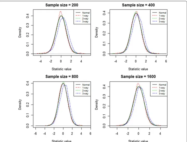
In Fig. 1, the null distributions for the one- and
two-way models followed the normal distribution quite closely, whereas the three-way model displayed a slight
sensitivity c, t|f (X) = Pr f (X) > c|δ(t) = 1 , specificity c, t|f (X) = Pr f (X) ≤ c|δ(t) = 0 ,
right skew. Nevertheless, the upper right tail regions almost perfectly overlapped with the upper right tail of the normal distribution for all three interaction mod-els. This showed that the use of the 95th quantile of the empirical distribution as a threshold to remove false pos-itives was suitable. This would greatly reduce the com-puting time by comparing testing scores with the prior calculated empirical distribution [14]. In Table 1, we used
the 95th quantile of data sets with 400 samples to esti-mate the type 1 error rate. The estiesti-mated rate for type I error was tightly distributed around 5% with a range from 4.5 to 5.6% for the one-way and two-way models. The estimated error rate for the three-way model was greater with a range from 7.5 to 9.7%; however, it also exhibited a trend towards 5% with increasing sample size. Based on the results in Table 1, simulation I revealed that with every two-fold increase in the sample size, there was an average 0.6% decrease in error rate for the three-way model. As a result, we expected that the type I error rate would converge to 5% with sample sizes greater than approximately 12,800.
Assessing power and speed in simulation II
In the second simulation, we estimated the power of ES-MDR with a data set that included quantitative out-come variables and a pair of functional interacting SNPs and 18 non-interacting SNPs. We determined whether Fig. 1 Empirical Distribution of the two-fold cross-validated testing scores. Each graph for sample sizes 200, 400, 800 and 1600 displays four curves
that represent the testing score distributions for a one-, two-, and three-way model and the standard normal distribution
Table 1 Estimated type I error rate in simulation i using the 95th quantile of the standard normal distribution
a m, number of SNPs; n, sample size
ma = 20 na = 200 (%) n a = 400 (%) n a = 800 (%) n a = 1600 (%) n a = 3200 (%) 1-way 4.5 4.7 4.9 4.8 5.0 2-way 5.3 5.6 5.2 5.4 5.4 3-way 9.7 8.7 8.1 7.5 7.8
the power of ES-MDR was comparable to Surv-MDR in identifying the two functional SNPs. We counted the number of times that the functional SNP pair was cor-rectly identified and divided that number by the total number of data sets (500 for this simulation) to get the estimated success rate.
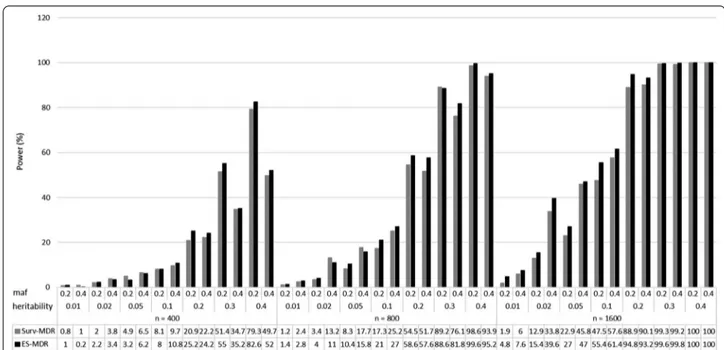
Figure 2 presents a comparison of the power to
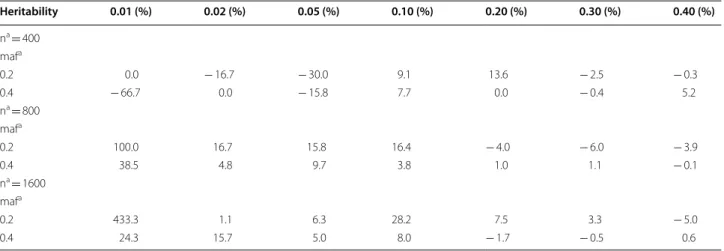
iden-tify only the two (i.e., stringent model) interacting SNPs (SNP1 and SNP2) for ES-MDR and Surv-MDR on simu-lated data. Table 2 displays the percent change in power
to detect only the two functional interacting SNPs between ES-MDR and Surv-MDR. Overall, ES-MDR performed better than Surv-MDR for larger sample sizes. In addition, both ES-MDR and Surv-MDR demonstrated increasing power to detect functional SNPs with increas-ing heritability frequencies.
Figure 3 displays a comparison in power to identify
the two interacting SNPs (SNP1 and SNP2) plus an addi-tional SNP (i.e., flexible model) between ES-MDR and
Surv-MDR. Table 3 shows the percent change in power
Fig. 2 Simulation II Power Comparison between ES-MDR and Surv-MDR – Stringent Model. The stringent model included two interacting SNPs (i.e.,
SNP1 and SNP2) and used n—sample sizes (e.g., 400, 800, 1600), maf—minor allele frequencies (e.g., 0.2, 0.4) and heritability statistics (e.g., 0.01, 0.02, 0.05, 0.1, 0.2, 0.3, 0.4)
Table 2 Percent change in power between ES-MDR and Surv-MDR
a n, sample size; maf, minor allele frequency;
b % change calculator = ((ES-MDR − Surv-MDR)/Surv-MDR) × 100%
Heritability 0.01 (%) 0.02 (%) 0.05 (%) 0.10 (%) 0.20 (%) 0.30 (%) 0.40 (%) na = 400 mafa 0.2 0.0 − 16.7 − 30.0 9.1 13.6 − 2.5 − 0.3 0.4 − 66.7 0.0 − 15.8 7.7 0.0 − 0.4 5.2 na = 800 mafa 0.2 100.0 16.7 15.8 16.4 − 4.0 − 6.0 − 3.9 0.4 38.5 4.8 9.7 3.8 1.0 1.1 − 0.1 na = 1600 mafa 0.2 433.3 1.1 6.3 28.2 7.5 3.3 − 5.0 0.4 24.3 15.7 5.0 8.0 − 1.7 − 0.5 0.6
to detect the two interacting SNPs plus an additional SNP. Here, we also demonstrated that ES-MDR had greater power compared to Surv-MDR. Again, ES-MDR performed better than Surv-MDR with larger sample sizes.
We compared the computing time between ES-MDR and Surv-MDR for 100 simulated data sets, for one-, two-, and three-way interactions, and with ten-fold cross-validation. The computing time for Surv-MDR was 734.5 min versus 2.25 min for ES-MDR, both of which
were run on 1 node in the high-performance comput-ing cluster called Discovery with AMD 3.1 Ghz CPU and 64 GB of memory. Discovery uses a Linux RedHat 6.7 operating system and is comprised of 160 computing nodes (3000 + cores), 12.5 TB of memory, and is available to the Dartmouth research community.
Application to OncoArray‑TRICL data set
The main goal was to identify SNPs with main effects and SNP interactions that were associated with lung Fig. 3 Simulation II Power Comparison between ES-MDR and Surv-MDR—Flexible Model. The flexible model included two interacting SNPs (i.e.,
SNP1 and SNP2) plus a third SNP3 and used n—sample sizes (e.g., 400, 800, 1600), maf—minor allele frequencies (e.g., 0.2, 0.4) and heritability statistics (e.g., 0.01, 0.02, 0.05, 0.1, 0.2, 0.3, 0.4)
Table 3 Percent change in power between ES-MDR and Surv-MDR
a n, sample size; maf, minor allele frequency;
b % change calculator = (ES-MDR − Surv-MDR)/Surv-MDR × 100%
Heritability 0.01 (%) 0.02 (%) 0.05 (%) 0.10 (%) 0.20 (%) 0.30 (%) 0.40 (%) na = 400 mafa 0.2 25.0 10.0 − 34.7 − 1.2 20.6 7.0 4.2 0.4 − 80.0 − 10.5 − 4.6 11.3 9.0 1.4 4.6 na = 800 mafa 0.2 16.7 17.6 25.3 21.4 7.5 − 0.7 1.0 0.4 16.7 − 16.7 − 10.7 7.1 11.4 7.5 1.4 na = 1600 mafa 0.2 152.6 19.4 17.9 16.6 6.6 0.3 0.0 0.4 26.7 17.2 2.6 6.6 3.4 0.6 0.0
cancer susceptibility at different ages of disease onset. Using a population-based study, we applied ES-MDR on the OncoArray-TRICL Consortium data with 14,935 cases and 12,787 controls for lung cancer to search over all one-way and two-way interactions to identify genetic interactions in relation to lung cancer age-of-onset. For this study, we included 533,631 genotyped variants and removed SNPs in linkage disequilibrium (LD) > 0.1 (n = 108,254 SNPs).
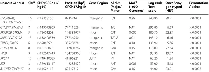
Table 4 lists the top 10 one-way test results generated by ES-MDR and cross-validation. Using ES-MDR, highly significant SNPs were identified in association with lung cancer age-of-onset. Table 5 displays the top 10 two-way interactions identified by ES-MDR that were associated with lung cancer age-of-onset. Due to the observed infla-tion of the type 1 error rate for 3-way interacinfla-tions in the simulation study, a 3-way interaction was not evaluated
in the OncoArray-TRICL data analysis. For Table 6, we
combined SNPs from the top 1000 one-way loci and the top 1000 two-way interactions, ranked the SNP scores from highest to lowest, and applied the Lasso Cox regres-sion method to filter and select the best genetic factors
that predicted age of lung cancer onset. Table 6
exhib-its the top 10 significant SNPs selected by Lasso Cox regression. To visualize the difference in age of lung cancer onset between the high risk and low risk groups,
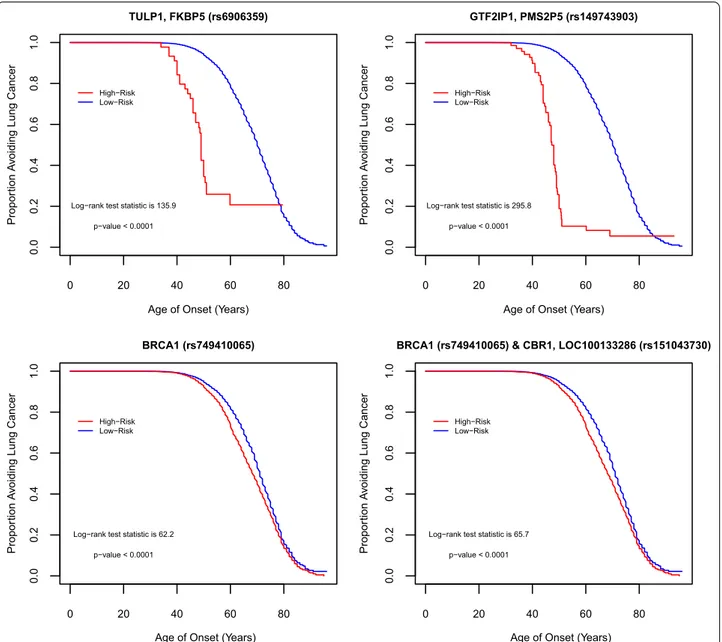
Fig. 4 illustrates the contrast using the KM) survival
curve. KM curves for top one-way SNPs in the intronic region of TULP1, FKBP5 (rs6906359), in-between genes GTF2IP1, PMS2P5 (rs149743903), and in the dele-tion of a noncoding region of BRCA1 (rs749410065) (NC_000017.10:g.41196821delT per Human Genome Variation Society nomenclature), and for a top two-way interacting SNPs in gene regions of BRCA1 (rs749410065) and CBR1, LOC100133286 (rs151043730)
displayed a clear separation of curves between the high- and low-risk groups. This demonstrated the efficacy of ES-MDR using Martingale Residuals to differentiate high risk and low risk groups based on genotype varia-tion when evaluating lung cancer age-of-onset. We con-tinued our analysis with a comparison of smoking only and smoking plus SNP models to determine the best performance in predicting lung cancer onset at different ages. We used a common graphical plot called the area under the receiver operating characteristic (ROC) curve, also known as AUC, to measure the performance of our models to discriminate the best parameters at predicting lung cancer onset at different ages based on accuracy. In
Fig. 5, the x-axis corresponds to the age of lung cancer
onset, starting from 15 to > 80 years, and the y-axis indi-cates the AUC, ranging from 0.4 to 1. We examined the predictive performance of 7 different models with vari-ous tuning parameters identified from Cox Lasso regres-sion, such as smoking only and smoking plus 2 SNPs, 4 SNPs, 13 SNPs, 19 SNPs, 29 SNPs, and 183 SNPs. This figure shows the average of the estimated AUCs over the OncoArray-TRICL data using the predictive scores from the independent left-out test data set. The plot displays good predictive performances of models generated using ES-MDR. The AUC for models with more SNPs lies between 0.6 and 0.7 and continues to increase at later ages of onset. There is a noticeable decrease in AUC for ages 40 and below. This could be due to the limited num-ber of lung cancer cases identified for individuals below the age of 40, which indicated that the models might not be appropriate to predict lung cancer diagnoses at 40 years and younger. The AUC of both smoking only and smoking with SNPs increased with age from age 40 and older. However, the AUC, depending on the number of SNPs in the models, differed by age. The model with the Table 4 Top-one-way models identified by ES-MDR in OncoArray-TRICL data
a Chr, chromosome; bp, base pair; MA, minor allele frequency; detT, NC_000017.10:g.41196821delT; NA, not available; HR, hazard ratio
Nearest Gene(s) Chra SNP (GRCh37/
hg19) Position (bp
a)
GRCh37/hg19 Gene Region Alleles (Major/ Minor) MAFa (1000 Genomes) Log‑rank Test score OncoArray‑ genotyped (HRa) Permutation P value LINC00708, LOC105755953 10 rs12358150 8735744 Intergenic C/T 0.26 340.90 20.51 < 0.0001 GTF2IP1, PMS2P5 7 rs149743903 74711828 Intergenic T/C NAa 295.80 6.39 < 0.0001 PPP2R2B, STK32A 5 rs76601208 146581977 Intron C/T 0.002 180.30 22.83 < 0.0001 KLF5, LINC00392 13 rs138428539 73736950 Intergenic T/C,G 0.01 145.10 6.46 < 0.0001 TULP1, FKBP5 6 rs6906359 35528378 Intron C/T 0.10 135.90 5.76 < 0.0001
UTP23, RAD21 8 rs10105870 117807762 Intergenic G/A 0.15 113.00 27.64 < 0.0001
VPS8 3 rs112047443 184701960 Intron A/T NAa 93.30 19.57 < 0.0001
BRCA1 17 rs749410065 41196821 delTa -/T NAa 62.20 1.24 < 0.0001
ATR 3 rs529613417 142285472 Intron A/T 0.001 57.00 5.48 < 0.0001
Table 5 T op t w o-w ay mo dels iden tified b y ES -MDR in O nc oA rr ay -TRICL da ta a UTR, un tr ansla ted r eg ion; delT a, NC_000017.10:g .41196821delT ; ncRNA, nonc oding tr anscr ipt v ar ian t; HR, hazar d r
atio; NA, not a
vailable G ene(s) 1 SNP 1 (GRC h37/ hg19) G
ene Region 1
A
lleles (Major/ Minor)
MA F a (1000 Genomes) G ene(s) 2 SNP 2 (GRC h37/ hg19) G
ene Region 2
A
lleles (Major/ Minor)
M AF (1000 G enomes) ES ‑MDR Test Sco re O nc oA rr ay ‑ genot yped (HR a) Log ‑r ank
test statistic
Permuta tion P v alue BR CA1 rs749410065 delT a –/T NA a CBR1, LOC100133286 rs151043730 missense , ncRNA a G/A 0.001 13.77 1.24 65.74 < 0.0001 BR CA1 rs749410065 delT a –/T NA a NAPG rs3865365 near 5 ′ end of genes G/A 0.06 13.43 1.23 61.74 < 0.0001 C6or f10 rs16870005 Intr on C/T 0.01 BR CA1 rs749410065 delT a –/T NA a 13.42 1.25 67.66 < 0.0001 C1or f21, LOC107985236 rs7535067 Intr on, 3 ′ UTR a C/A,T 0.19 BR CA1 rs749410065 delT a –/T NA a 13.39 1.24 61.92 < 0.0001 PSMB9, LOC100294145 rs57092860 Int er genic T/C,G 0.01 BR CA1 rs749410065 delT a –/T NA a 13.37 1.25 67.82 < 0.0001 CTNND2 rs7732411 Intr on T/C 0.08 BR CA1 rs749410065 delT a –/T NA a 13.32 1.25 67.53 < 0.0001 TRAM2-A S1, LOC730101 rs182398206 Int er genic A/G 0.01 BR CA1 rs749410065 delT a –/T NA a 13.30 1.25 70.95 < 0.0001 MIR4417, MIR4689 rs6698924 Int er genic A/C 0.02 BR CA1 rs749410065 delT a –/T NA a 13.29 1.25 68.74 < 0.0001 BR CA1 rs749410065 delT a –/T NA a TF AP2C, BMP7 rs186132350 Int er genic T/A 0.01 13.29 1.25 69.79 < 0.0001 HRA T92, PRK AR1B rs142263110 Int er genic G/A 0.002 BR CA1 rs749410065 delT a –/T NA a 13.28 1.25 69.36 < 0.0001
largest number of SNPs plus smoking performed the best at AUC 0.68 between ages 40 and 80 of onset compared to the smoking-only model with an AUC of 0.55. There was a noticeable trend where incremental additions of SNPs in the model increased the AUC for age-of-onset between 40 and 80 + . On the other hand, the AUC for smoking-only and smoking plus fewer SNP models (e.g., 2 and 4) displayed the opposite trend where it increased around 90 + years of age.
Discussion
In this study, we present a novel algorithm to identify genetic interactions associated with the age-of-onset for lung cancer. We demonstrated in two simulation studies that our ES-MDR method was properly controlled for at the 5% type I error rate under the null distribution and improved power to detect causal SNPs. We identified new loci that were biologically plausible for lung cancer onset using the large OncoArray-TRICL data with 27,722 individuals. There are two unique contributions from this study. First, we offer a more computationally efficient algorithm, ES-MDR, a method that analyses survival data by using Martingale residuals in place of survival outcome data. Second, ES-MDR includes the ability to adjust for covariates, such as smoking status, a necessary step to control for confounding factors, whereas existing methods, used for survival analysis such as Surv-MDR, are unable to provide.
Using the MDR method to reduce the size of multiple dimensions to a single dimension to identify multi-locus genetic interactions in high-dimensional genomic data sets has been a well-established approach. Richie et al. (2001) first introduced MDR, a non-parametric (i.e., no parameters are estimated) and genetic model-free (i.e., no genetic model is assumed) model, that condensed
multiple genetic loci into a single variable in order to cat-egorize genotypes into two groups [7]. The goal was to group genotypes into high-risk and low-risk categories associated with and without disease outcomes, respec-tively. However, MDR was restricted by its inability to analyze different outcome variables other than binary variables and it did not allow for the adjustment of con-founding factors that was critical in preventing false association analyses. Therefore, an extension of the tradi-tional MDR method was developed to analyze censored survival data, called Survival MDR or Surv-MDR.
Like the original MDR algorithm, Surv-MDR is a non-parametric and genetic model-free method proposed by Gui et al. (2011), and it was developed to allow for the analysis of time-to-event data, such as patient survival time or time to disease relapse [13]. Surv-MDR used the log-rank test statistic to compare survival times between samples with and without the multi-locus risk genotype combination and classified them into high and low risk groups [13]. Surv-MDR also used cross-validation to identify the optimal set of K SNPs and overall best model. While Surv-MDR was successful in identifying SNP interactions associated with time-to-event outcomes, it was more computationally demanding than MDR and the inability to adjust for covariates persisted. Consequently, the MDR method was optimized further to develop the Quantitative MDR (QMDR) method to address the slow-to-compute algorithm challenge [14].
QMDR optimized the MDR algorithm by offering a computationally efficient way to analyze quantitative or continuous trait outcomes. QMDR compared the mean value of each multi-locus genotype to the overall mean and labeled each genotype combination as “high-risk” or “low-risk”. Cross-validation was also implemented in QMDR to identify the optimal set of K SNPs and overall Table 6 Top SNPs selected by cox lasso regression in OncoArray-TRICL data
a Chr, chromosome; NA, not available; bp, base pair; delTa = NC_000017.10:g.41196821delT; MAF, minor allele frequency; HR, hazard ratio
Nearest Gene(s) Chra SNP (GRCh37/
hg19) Position (bp
a)
(GRCh37/ hg19)
Gene region Alleles (Major/ Minor)
MAFa
(1000 Genomes)
Test score OncoArray‑ genotyped (HRa) Permutation P value BRCA1 17 rs749410065 41196821 delTa –/T NAa 62.20 1.24 < 0.0001 GTF2IP1, PMS2P5 7 rs149743903 35528378 Intergenic C/G NAa 295.80 6.39 < 0.0001 LOC102467079, TOX3 16 rs117142114 52328666 Intergenic T/C 0.02 31.00 1.29 < 0.0001 HYKK 15 rs9788721 78802869 Intron C/T 0.31 86.30 1.41 < 0.0001
MIR3925, PANDAR 6 rs7753169 36614326 Intergenic A/C 0.36 27.90 1.15 < 0.0001
CHRNA5 15 rs16969968 78882925 missense G/A 0.15 86.80 1.41 < 0.0001
KLF5, LINC00392 13 rs138428539 73736950 Intergenic T/C,G 0.01 145.10 6.46 < 0.0001
TULP1, FKBP5 6 rs6906359 35528378 Intron C/T 0.10 135.90 5.76 < 0.0001
CHRNA5 15 rs951266 78878541 Intron G/A 0.16 88.50 1.41 < 0.0001
best model. For each K-way interaction, the steps used for a k-fold cross-validation were similar to the Surv-MDR method except for the step to identify the best K-way interaction. In this case, the largest T-test tic was used instead of the square of the log-rank statis-tic when identifying the best interaction model. Inspired by the computational capabilities of QMDR to analyze quantitative outcomes associated with genetic variations, we leveraged this method’s straightforward computing efficiency to evaluate survival outcome data for time-to-event analysis.
Our approach transformed survival data (e.g., time and event status) into a single variable, Martingale Residu-als, to use as a surrogate for time-to-disease and disease status, with application of QMDR for rapid processing of genotype combinations into high and low risk groups. We were able to identify thousands of significant one-way and two-way models using ES-MDR and cross-validation when applied to the lung cancer OncoArray-TRICL data set. We were unable to compare the results of ES-MDR and Surv-MDR, both because Surv-MDR would have taken an extensive amount of time (e.g., greater than
0 20 40 60 80 0. 0 0. 20 .4 0. 60 .8 1. 0 TULP1, FKBP5 (rs6906359)
Age of Onset (Years)
Propor
tion
Av
oiding Lung Cancer
Log−rank test statistic is 135.9 p−value < 0.0001 High−Risk Low−Risk 0 20 40 60 80 0. 0 0. 20 .4 0. 60 .8 1. 0 GTF2IP1, PMS2P5 (rs149743903)
Age of Onset (Years)
Propor
tion
Av
oiding Lung Cancer
Log−rank test statistic is 295.8 p−value < 0.0001 High−Risk Low−Risk 0 20 40 60 80 0. 0 0. 20 .4 0. 60 .8 1. 0 BRCA1 (rs749410065)
Age of Onset (Years)
Propo
rtion
Av
oiding Lung Cancer
Log−rank test statistic is 62.2 p−value < 0.0001 High−Risk Low−Risk 0 20 40 60 80 0. 0 0. 2 0. 40 .6 0. 8 1. 0
BRCA1 (rs749410065) & CBR1, LOC100133286 (rs151043730)
Age of Onset (Years)
Propo
rtion
Av
oiding Lung Cancer
Log−rank test statistic is 65.7 p−value < 0.0001
High−Risk Low−Risk
Fig. 4 Differences between High Risk (red curve) and Low Risk (blue curve) groups in relation to SNPs. Kaplan–Meier plots displays the difference
between individuals categorized in High Risk vs. Low Risk groups by genetic variation in top one-way SNPs identified from the testing set, TULP1/ FKBP5 (rs6906359), GTF2IP1/PMS2P5 (rs149743903), and BRCA1 (rs749410065) (NC_000017.10:g.41196821delT), and in a top two-way interacting SNPs from the testing set, BRCA1 (rs749410065) (NC_000017.10:g.41196821delT) & CBR1, LOC100133286 (rs151043730)
4 months) to conduct a genome-wide genetic interac-tion analysis using the large OncoArray-TRICL data set, and because the current Surv-MDR algorithm would not allow for adjustment of confounding factors such as smoking status.
When searching for SNP interactions using real data, we chose a two-fold cross-validation instead of a ten-fold cross-validation to evaluate the optimal one-way and two-way interaction models as described previously [14]. From the central limit theorem, assuming a sufficiently large sample size (n > 50) from a population with a finite level of variance, the mean of all samples from the same population would be approximately equal to the mean of the population. Therefore, we expected the testing scores with 400 samples from our simulation study to follow a standard normal distribution. However, Gui et al. (2013) displayed a slight right skew with a standard deviation of 1.6 in their empirical distributions that was due to extra variation introduced by overlapping training sets in their
ten-fold cross-validation method [14, 21]. Furthermore,
two-fold cross-validation had been advocated to perform hypothesis testing where the training folds were mutu-ally independent with no overlap [21]. Consequently,
we evaluated the optimal one-way and two-way interac-tion models and the overall best model using two-fold cross-validation.
We explored prediction models that included SNPs that could be used to forecast lung cancer onset. Figure 5 lays out the AUC estimates for each model. The AUC peaked around age-of-onset less than 30 and greater than 90 years old. This may be due to the limited number of lung cancer cases (e.g., less than 10 cases) at younger and older ages. In general, based on AUC averages, age of lung cancer onset was strongly influenced by genetic variants, with increasing numbers of SNPs contributing to better AUC estimates. The plateauing of AUC averages for the 40–80 years old range revealed good estimates for age of onset for all models, which was likely due to the larger sample size for evaluation. Another plausible explanation for the high AUC for early and late age of onset was the likelihood that those cases contained the same combina-tions of risk SNPs in the models. The identified top SNPs with high AUC for age of onset were not only associated with early lung cancer cases, but they potentially could also contribute to late age of onset cases. The 2 SNP and 4 SNP models had strong associations with lung cancer Fig. 5 Plots of Area under the curve (AUC). Each line corresponds to a model. Models were smoking only and smoking plus 2 to 183 SNPs. Here we
compared the AUCs between the smoking only model and smoking plus SNPs models for predicting lung cancer age-of-onset ranging from 20 to < 100 years. The number of individuals diagnosed with lung cancer at < 40 years, 40 to < 60 years, 60 to < 80 years, and 80 to < 100 years is shown below the figure
cases and therefore, were responsible for high AUC aver-ages for early and late age of onset of lung cancer. For the smoking only model, it played less of a role for early lung cancer onset because the adverse effects from smoking could require more time to develop. Over time the effects from smoking could be the main driver for late age lung cancer cases, which could explain why genetic factors do not seem to greatly effect cancer onset in later years. This interpretation could make biological sense since the effect of smoking over a longer time period could have compounding effects on cancer development. Con-versely, cancer development due to genetics might appear at earlier rather than later years.
Limitations
While our novel ES-MDR overcame some of the limita-tions described in previous methods used to evaluate genetic interactions, it was not without some of its own disadvantages. When analyzing survival data, the method did not directly evaluate survival variables such as time and event status. As a result, when using Martingale Residuals instead of specific survival outcomes data, we might be missing some important information that was needed to identify associations between SNP interac-tions and survival outcomes. Our QQ plot analysis from real data indicated a strong departure from the null dis-tribution which indicated that there might exist a sys-tematic bias. This result could be due to a combination of the large sample size and continuous outcome. As a result, we used permutation tests to evaluate the results from the OncoArray-TRICL data set. Another limita-tion came from over parameterizing our models, result-ing in many multifactor cells with missresult-ing data [7]. This did not affect the classification of genotype combinations or identifying cross-validation consistency of the model, however, it could affect our estimation of the prediction error [7]. Future studies would need to address this limi-tation. Next, we applied our ES-MDR method to analyze survival outcomes using case–control studies, where estimating the age-specific incidence (e.g., age-of-onset) was not typically designed for case–control studies. On the other hand, cohort studies, which are designed for survival analyses, are expensive and require a great deal of follow-up time to obtain age-of-onset information. This could be one of the barriers in analyzing survival outcomes for large cohort studies; it could require a lot of time and resources to amass an extensive amount of data. In our study, we were able to analyze and identify potential genetic markers that predicted lung cancer risk using a large lung cancer GWAS consortium data, which could be followed up with further investigations for bio-logical and functional significance. Due to fewer available observations of lung cancer age-of-onset among younger
individuals, we were limited in our ability to predict lung cancer onset for individuals 40 years and younger. With continuous efforts in recruiting participants in the OncoArray-TRICL Consortium, we might find more cases among the early onset population to better pre-dict lung cancer risk in the future. Finally, there were no available validation data to replicate our top SNP findings because these SNPs were not likely genotyped in other GWAS data sets. Currently, there are ongoing efforts to collect external data that will include genotyping of our top SNP findings for replication.
Future studies
ES-MDR is a powerful alternative to Surv-MDR for identifying interactions, especially at the genome-wide scale. We demonstrated its ability to identify high-order genetic interactions in simulated and real data sets. Although ES-MDR addresses previous limitations of Surv-MDR and other MDR-like methods, there are ways in which this method can be improved. While ES-MDR had greatly improved computing efficiency, genome-wide scans for interactions will still require massive computing resources, especially to analyze higher-order interactions. It will be necessary to optimize the selection of SNPs in predictive models, for example, by selecting genes known to participate in biological and metabolic pathways [22]. This can improve the predictive ability of ES-MDR for two-, three, and multi-way interactions in a pathway analysis. Second, a future study may entail introducing variance back to Martingale Residuals by way of weight-ing each residual based on the time-to-event data. This can greatly improve our power for model selection with-out removing the efficiency of the algorithm.
Conclusions
In summary, the ES-MDR method provides a way to ana-lyze high-order interactions at the genome-wide scale to advance studies of genetic interactions. We developed a new method that efficiently captures non-linear and high-order interactions for time-to-event analysis.In gen-eral, ES-MDR has improved power performance relative to Surv-MDR using simulated data. Based on the noticea-ble trends, we are confident that with bigger sample sizes, ES-MDR will continue to significantly gain in power to detect functional interacting SNPs without inflating the type I error rate. Providing new and improved methods to analyze epistasis or gene interactions may offer new opportunities to not only explain the missing heritability for complex disease risk, but can also potentially detect new genetic determinants that is important for clinical utility such as disease diagnosis and prognosis.
Abbreviations
GWAS: Genome-wide association studies; SNP: Single nucleotide polymor-phism; ES-MDR: Efficient Survival Multifactor Dimensionality Reduction; HR: Hazard ratio; MDR: Multifactor Dimensionality Reduction; Surv-MDR: Survival MDR; QMDR: Quantitative MDR; TRICL: Transdisciplinary Research Into Cancer of the Lung; MAF: Minor allele frequency; Cox ph: Cox proportional hazards; GHz: Gigahertz; CPU: Central processing unit; GB: Gigabyte; TB: Terabyte; Lasso: Least absolute shrinkage and selection operator; ROC: Receiver operating characteristic; AUC : Area under the ROC curve; bp: Base pair; ncRNA: Noncod-ing transcript variant; UTR : Untranslated region.
Acknowledgements
The authors would like to thank all members of the Transdisciplinary Research in Cancer of the Lung (TRICL) Consortium for their data collection that made this study possible.
Authors’ contributions
J.G. and C.I.A. contributed to the project design and oversight. J.G. contributed to the method development. J.G. and J.L. contributed to the implementa-tion and benchmarking. J.L. and X.J. wrote the manuscript. J.G., C.I.A., J.L., X.J., T.A.M., and S.L. contributed to the data analysis and discussions. X.J., X.X., and J.L. contributed to the genetic annotation of identified genes. J.G., C.I.A., and J.L. contributed to the data interpretation. J.L., X.J., S.L., X.X., D.Z., E.J.D., D.C.C., M.B.S., S.M.A., S.Z., H.B., O.M., M.D.T., T.A.M., C.I.A., and J.G. contributed to the data preparation, manuscript editing, and discussion. All authors read and approved the final manuscript.
Funding
This publication was funded in part by the following: National Institute of Health (NIH), National Library of Medicine (NLM) Institute research grants R01LM012012 and T32LM012204, National Cancer Institute (NCI) grant U19CA203654, and the Cancer Prevention Research Institute of Texas (CPRIT) RR170048. NIH-NLM R01LM012012, NCI U19CA203654 and CPRIT RR170048 funded the design, data collection, analysis and interpretation of the study and in writing the manuscript. NIH-NLM T32LM012204 funded the analysis and interpretation of the data and in writing the manuscript.
Availability of data and materials
The datasets generated and/or analyzed during the current study are avail-able in the NCBI dbGaP repository, dbGaP Study Accession: phs001273.v3.p2, website: https ://www.ncbi.nlm.nih.gov/proje cts/gap/cgi-bin/study .cgi?study _id=phs00 1273.v3.p2.
Ethics approval and consent to participate
The Dartmouth-Hitchcock Health Institutional Review Board (D-HH IRB) at the Office of Research Operations at Dartmouth-Hitchcock reviewed and approved the study protocols and data analysis for the research titled: “Genome-Wide Association Study of Common Cancers—The GAME-ON Con-sortium (ONCOCHIP)”, IRB ID: CR00006213. All participants provided written informed consent and each study site approved the study protocols and data analysis from their local ethics committees.
Consent for publication Not applicable. Competing interests
The authors declare that they have no competing interests. Author details
1 Quantitative Biomedical Science Program, Geisel School of Medicine, Dart-mouth College, Hanover, NH 03755, USA. 2 Department of Biomedical Data Science, Geisel School of Medicine, Dartmouth College, One Medical Center Dr., Lebanon, NH 03756, USA. 3 Institute for Clinical and Translational Research, Dan L. Duncan Comprehensive Cancer Center, Baylor College of Medicine, Houston, TX 77030, USA. 4 Unit of Nutrition and Cancer, Catalan Institute of Oncology (ICO-IDIBELL), 08908 Barcelona, Spain. 5 Department of Environmental Health, Harvard School of Public Health, Boston, MA 02115, USA. 6 Department of Medicine, Massachusetts General Hospital, Boston, MA 02115, USA. 7 Department of Cancer Epidemiology, H. Lee Moffitt Cancer Center and Research Institute, Tampa, FL 33612, USA. 8 Markey Cancer Center, University of Kentucky, First Floor, 800 Rose Street, Lexington, KY 40508, USA. 9 National Institute of Occupational Health, 0033 Gydas vei 8, 0033 Oslo, Norway. 10 Laboratory Medicine Region Skåne,
Department of Clinical Sciences Lund, Pathology, Lund University, Lund, Sweden. 11 Department of Clinical Sciences, Lund University, Malmö, Sweden. 12 Division of Public Health Sciences, Fred Hutchinson Cancer Research Center, Seattle, WA 98109, USA.
Received: 16 September 2019 Accepted: 11 October 2020
References
1. Manolio TA, Collins FS, Cox NJ, Goldstein DB, Hindorff LA, Hunter DJ, McCarthy MI, Ramos EM, Cardon LR, Chakravarti A, et al. Finding the missing heritability of complex diseases. Nature. 2009;461:747–53.
2. Hirschhorn JN, Daly MJ. Genome-wide association studies for common diseases and complex traits. Nat Rev Genet. 2005;6:95–108.
3. McCarthy MI, Abecasis GR, Cardon LR, Goldstein DB, Little J, Ioannidis JP, Hirschhorn JN. Genome-wide association studies for complex traits: consen-sus, uncertainty and challenges. Nat Rev Genet. 2008;9:356–69.
4. Bush WS, Moore JH. Chapter 11: Genome-wide association studies. PLoS Comput Biol. 2012;8:e1002822.
5. Maher B. Personal genomes: the case of the missing heritability. Nature. 2008;456:18–21.
6. Gilbert-Diamond D, Moore JH. Analysis of gene-gene interactions. Curr Protoc Hum Genet. 2011;Chapter 1:Unit1 14.
7. Ritchie MD, Hahn LW, Roodi N, Bailey LR, Dupont WD, Parl FF, Moore JH. Multifactor-dimensionality reduction reveals high-order interactions among estrogen-metabolism genes in sporadic breast cancer. Am J Hum Genet. 2001;69:138–47.
8. Moore JH, Williams SM. Epistasis and its implications for personal genetics. Am J Hum Genet. 2009;85:309–20.
9. Park MY, Hastie T. Penalized logistic regression for detecting gene interac-tions. Biostatistics. 2008;9:30–50.
10. Andrew AS, Gui J, Sanderson AC, Mason RA, Morlock EV, Schned AR, Kelsey KT, Marsit CJ, Moore JH, Karagas MR. Bladder cancer SNP panel predicts susceptibility and survival. Hum Genet. 2009;125:527–39.
11. He H, Oetting WS, Brott MJ, Basu S. Power of multifactor dimensionality reduction and penalized logistic regression for detecting gene-gene inter-action in a case-control study. BMC Med Genet. 2009;10:127.
12. Moore JH, Asselbergs FW, Williams SM. Bioinformatics challenges for genome-wide association studies. Bioinformatics. 2010;26:445–55. 13. Gui J, Moore JH, Kelsey KT, Marsit CJ, Karagas MR, Andrew AS. A novel
sur-vival multifactor dimensionality reduction method for detecting gene-gene interactions with application to bladder cancer prognosis. Hum Genet. 2011;129:101–10.
14. Gui J, Moore JH, Williams SM, Andrews P, Hillege HL, van der Harst P, Navis G, Van Gilst WH, Asselbergs FW, Gilbert-Diamond D. A simple and computa-tionally efficient approach to multifactor dimensionality reduction analysis of gene-gene interactions for quantitative traits. PLoS ONE. 2013;8:e66545. 15. Brandt A, Bermejo JL, Sundquist J, Hemminki K. Age of onset in familial
cancer. Ann Oncol. 2008;19:2084–8.
16. Dietterich TG. Approximate statistical tests for comparing supervised clas-sification learning algorithms. Neural Comput. 1998;10:1895–923. 17. Amos CI, Dennis J, Wang Z, Byun J, Schumacher FR, Gayther SA, Casey G,
Hunter DJ, Sellers TA, Gruber SB, et al. The OncoArray consortium: a network for understanding the genetic architecture of common cancers. Cancer Epidemiol Biomarkers Prev. 2017;26:126–35.
18. Gui J, Li H. Penalized Cox regression analysis in the high-dimensional and low-sample size settings, with applications to microarray gene expression data. Bioinformatics. 2005;21:3001–8.
19. Tibshirani R. The lasso method for variable selection in the Cox model. Stat Med. 1997;16:385–95.
20. Heagerty PJ, Lumley T, Pepe MS. Time-dependent ROC curves for censored survival data and a diagnostic marker. Biometrics. 2000;56:337–44. 21. Bengio Y, Grandvalet Y. No unbiased estimator of the variance of k-fold
cross-validation. J Mach Learn Res. 2004;5:1089–105.
22. Wang K, Li M, Hakonarson H. Analysing biological pathways in genome-wide association studies. Nat Rev Genet. 2010;11:843–54.
Publisher’s Note
Springer Nature remains neutral with regard to jurisdictional claims in pub-lished maps and institutional affiliations.