Development of best estimate numerical tools for LFR design and safety analysis

(1)

Ricerca Sistema Elettrico

Sigla di identificazione ADPFISS – LP2 – 158 Distrib. L Pag. di 1 213 Titolo

Development of best estimate numerical tools for LFR

design and safety analysis

Descrittori

Tipologia del documento: Rapporto Tecnico

Collocazione contrattuale: Accordo di programma ENEA-MSE su sicurezza nucleare e Reattori di IV generazione

Argomenti trattati: Reattori Nucleari Veloci, Termoidraulica dei reattori nucleari Sicurezza nucleare, Analisi incidentale

Sommario

Nell’ambito della linea LP2, sono state condotte attività di ricerca al fine di sviluppare, aggiornare e convalidare codici di calcolo e modelli numerici per sostenere la progettazione ed effettuare analisi di sicurezza di un reattore veloce refrigerato a metallo liquido. Nell’ambito del PAR 2016, sono state messe in atto delle azioni al fine di integrare e coordinare tali attività. Si sono, pertanto, definite le aree di simulazione e le interconnessioni rilevanti per la progettazione e sicurezza di reattori Gen-IV. Il presente report rappresenta il proseguimento di tale azione. Ognuna di queste aree di simulazione è coperta da uno o più codici e simula un set di fenomeni multi-fisica e multi-scala rilevanti, e.g. termoidraulica di sistema, di contenimento, di sotto-canale, fluidodinamica tridimensionale, termo-meccanica della barretta di combustibile, del fuel assembly e di componenti, generazione di sezioni d’urto e sviluppo di metodi di aggiustamento delle stesse mediante utilizzo di dati sperimentali, dinamica neutronica tridimensionale, rilascio e trasporto di prodotti di fissione, etc. Tale attività fa parte di un’azione di sviluppo e convalida di una piattaforma di calcolo per sistemi nucleari innovativi, che si dovrà protrarre nel PT2018- 2020 (e successivi).

Relativamente a sviluppo e convalida, riportate nella parte 2 del presente report, sono state effettuate attività relative a: 1. termo-meccanica della barretta di combustibile – supporto allo sviluppo del codice TRANSURANUS.

2. termoidraulica di sistema – supporto alla validazione del codice RELAP5-3D per applicazione ai sistemi a piscina 3. accoppiamento codici CFD/SYS-TH e loro validazione a fronte delle campagne sperimentali TALL

4. dinamica accoppiata neutronica-termoidraulica tridimensionale - sviluppo e applicazione codice FRENETIC 5. modellazione multifisica neutronica – termoidraulica - accoppiamento OpenFoam-Serpent

6. termoidraulica multifluid/multiphase e analisi di incidenti severi – supporto allo sviluppo e alla vlidazione del codice SIMMER-III e -IV

Note:

--Autori: T. Barani, A. Cammi, C. Castagna, L. Cognini, S. Lorenzi, L. Luzzi, A. Magni, D. Pizzocri (POLIMI) N. Abrate, S. Dulla, E. Guadagni, G. F. Nallo, P. Ravetto, L. Savoldi, D. Valerio, R. Zanino (POLITO) A. Chierici, L. Chirco, R. Da Vià, F. Franceschini, V. Giovacchini, S. Manservisi (UNIBO)

N. Forgione, B. Gonfiotti, C. Ulissi, M. Eboli (UNIPI)

G. Caruso, L. Ferroni, M. Frullini, F. Giannetti, L. Gramiccia, V. Narcisi, A. Subioli (UNIROMA1) A. Cervone, A. Del Nevo, I. Di Piazza, M. Tarantino (ENEA)

Copia n. In carico a:

1 NOME

FIRMA

0 _EMISSIONE _27/11/2018 NOME A. Del Nevo M. Utili M. Tarantino

(2)

(3)

Title: Development of BE numerical tools for LFR design and safety analysis

Project: ADP ENEA-MSE PAR 2017

Distribution PUBLIC Issue Date 27.11.2018 Pag. RICERCA SISTEMA ELETTRICO Ref. ADPFISS-LP2-158 Rev. 0

3 di 213

L

IST OF

R

EVISIONS

Revision

Date

Scope of revision

Page

(4)

4 di 213

(5)

5 di 213

L

IST OF CONTENTS

L

IST OF

R

EVISIONS

... 3

L

IST OF FIGURES

... 9

L

IST OF TABLES

... 15

L

IST OF ABBREVIATIONS

... 17

F

OREWORD

... 19

1 T

HERMO

-M

ECHANICS OF THE FUEL PIN

–

DEVELOPMENT AND ASSESSMENT OF MODELS AND ALGORITHMS DESCRIBING INERT GAS BEHAVIOR FOR USE IN

TRANSURANUS ... 21

1.1 Background and references ... 23

1.1.1 Helium solubility ... 23

1.1.2 PolyPole-2 algorithm ... 23

1.2 Body of the report concerning the ongoing activities ... 24

1.2.1 Helium solubility ... 25

1.2.2 PolyPole-2 algorithm ... 26

1.3 Role of the activity, general goals and future development ... 29

1.4 List of References ... 34

2 V

ALIDATION OF

RELAP53D

BY

CIRCE-ICE

EXPERIMENTAL TESTS

... 39

2.1 Background and references ... 41

2.2 Body of the report concerning the ongoing activities ... 42

2.2.1 CIRCE-ICE facility ... 42 2.2.2 Experimental test ... 43 2.2.3 Thermal-hydraulic model ... 43 2.2.4 Simulation results ... 45

2.3 Conclusive remarks ... 47

2.4 List of References ... 67

3 A

PPLICATION OF

RELAP5-3D

ON

PHENIX

EXPERIMENTAL TESTS

... 71

3.1 Background and references ... 73

(6)

6 di 213

3.2.5 Nodalization sensitivity: 1D model ... 78

3.3 Conclusive remarks ... 79

3.4 List of References ... 99

4 V

ALIDATION OF

FEM-LCORE

/

CATHARE

BY

TALL

3D

EXPERIMENTAL TESTS

... 101

4.1 Introductory remarks ... 103

4.1.1 The OpenFOAM-Salome-FemLCore-Cathare computational platform for LFR... 103

4.2 Validation of the platform coupling model by TALL-3D facility experimental tests ... 103

4.2.1 TALL-3D facility ... 103

4.2.2 Thermohydraulics model of the TALL-3D facility. ... 105

4.2.3 Simulations of the semi-blind test case TG03S301(03) ... 109

4.3 Conclusive remarks ... 113

4.4 List of References ... 133

5 T

HREE

-

DIMENSIONAL NEUTRONIC

-

THERMAL

-

HYDRAULIC DYNAMICS MODELLING

:

SERPENT-OPENFOAM-FRENETIC

COMPARISON AND APPLICATION TO

ALFRED

DESIGN

... 135

5.1 Introduction ... 137

5.2 Benchmark of FRENETIC against Serpent-OpenFOAM ... 138

5.2.1 NE-TH coupling and simulation strategy ... 138

5.2.2 FRENETIC-Serpent (NE) comparison ... 139

5.2.3 FRENETIC- OpenFOAM comparison ... 140

5.3 FRENETIC model for ALFRED ... 140

5.3.1 Serpent-2 model for multi-group nuclear data evaluation ... 140

5.3.2 Energy collapsing and spatial homogenization procedures in Serpent-2 ... 141

5.3.3 Temperature dependence of cross section ... 142

5.3.4 Steady-state results of the FRENETIC model for the ALFRED reactor ... 142

5.4 Conclusive remarks ... 144

List of References ... 157

6 MONTE

CARLO

–

CFD

COUPLING

FOR

LFR

MULTIPHYSICS

MODELLING ... 159

6.1 Background and references ... 161

6.1.1 Monte Carlo - CFD coupling ... 161

6.2 Body of the report concerning the ongoing activities ... 162

6.2.1 Monte Carlo – CFD coupling techniques ... 162

6.2.2 Full core SERPENT model of the ALFRED reactor ... 165

6.2.3 CFD model for the FA of ALFRED ... 166

6.2.4 SERPENT – OpenFOAM coupling for one-sixth of FA ... 167

(7)

7 di 213

7 SIMMER

III-RELAP5

COUPLING

CODES

DEVELOPMENT ... 179

7.1 Background and references ... 181

7.2 Body of the report concerning the ongoing activities ... 181

7.2.1 Principles of the coupling tool ... 181

7.2.2 Assessment of the coupling capabilities – Simple test cases ... 182

7.2.3 Assessment of the coupling capabilities – LIFUS5 facility ... 183

7.2.4 The RELAP5/Mod3.3 and the SIMMER III simplified nodalizations ... 183

7.2.5 LIFUS5/Mod3 coupled codes preliminary simulation results ... 184

7.3 Role of the activity, general goals and future development ... 184

7.4 List of References ... 199

8 F

UEL

-

COOLANT CHEMICAL INTERACTION

... 201

8.1 Introduction ... 203

8.2 Computational activities ... 203

8.2.1 Thermodynamic predictions by CALPHAD method ... 203

8.2.2 Integration of thermodynamic calculations in multi-physics codes ... 203

8.3 Experimental activities ... 204

8.4 Conclusive remarks ... 206

8.5 List of References ... 212

(8)

8 di 213

(9)

9 di 213

L

IST OF FIGURES

Fig. 1.1 – Plot of the experimental Henry's constant of helium in oxide fuel classified depending on the microstructure of the sample (i.e., blue for the powder samples and red for the single crystal

samples). Each cluster is fitted by a distinct correlation (dark red and dark blue) [1.45] ... 31

Fig. 1.2 – Comparison between intra-granular fission gas release calculated by the reference algorithm for the general PDE system (non-equilibrium) and the PolyPole-2 results – red points – and the FD results for the quasi-stationary approximation (equilibrium) – black points –. Each data point corresponds to a calculation with randomly generated RIA conditions. The distance from the 45° dashed line is a graphical measure of accuracy [1.44] ... 32

Fig. 1.3 – Comparison between the computational times associated with the FD and PolyPole-2 algorithms for the solution of the general PDE system. Each data point corresponds to a calculation with randomly generated RIA conditions [1.44] ... 33

Fig. 2.1 – CIRCE isometric view ... 49

Fig. 2.2 – ICE test section ... 49

Fig. 2.3 – ICE test section: primary flow path ... 50

Fig. 2.4 – FPS cross section ... 51

Fig. 2.5 – HX bayonet tube ... 51

Fig. 2.6 – CIRCE instrumentation: FPS (1) ... 52

Fig. 2.7 – CIRCE instrumentation: FPS (2) ... 53

Fig. 2.8 – CIRCE instrumentation: pool ... 54

Fig. 2.9 – Nodalizzation scheme: mono-dimensional model ... 55

Fig. 2.10 – Nodalizzation scheme: multi-dimensional model ... 56

Fig. 2.11 – Nodalizzation scheme: FPS ... 56

Fig. 2.12 – Power supplied ... 57

Fig. 2.13 – Feed-water mass flow rate ... 57

Fig. 2.14 – Argon injection ... 57

Fig. 2.15 – Air mass flow rate ... 57

Fig. 2.16 – LBE mass flow rate ... 58

Fig. 2.17 – FPS inlet/outlet temperature ... 58

Fig. 2.18 – HX inlet/outlet temperature ... 58

Fig. 2.19 – DHR inlet/outlet temperature ... 58

Fig. 2.20 – TS and MC: 3300 s... 59

Fig. 2.21 – TS and MC: 10000 s... 60

(10)

10 di 213

Fig. 2.25 – TS and MC: 60000 s... 64 Fig. 2.26 – TS and MC (1) ... 65 Fig. 2.27 – TS and MC (2) ... 66 Fig. 2.28 – FPS Temperature ... 67

Fig. 3.1 – Reactor block ... 82

Fig. 3.2 – Intermediate heat exchanger ... 82

Fig. 3.3 – Reactor top view ... 82

Fig. 3.4 – Primary pump ... 83

Fig. 3.5 – Vessel cooling system flow path ... 83

Fig. 3.6 – Reactor core top view ... 84

Fig. 3.7 – Fuel and fertile SA axial composition ... 84

Fig. 3.8 – Overview of radial and azimuthal meshes of MULTID component ... 85

Fig. 3.9 – Scheme of MULTID component for porosity factor ... 85

Fig. 3.10 – SAs inlet area (m2) ... 86

Fig. 3.11 – SAs inlet K loss ... 86

Fig. 3.12 – Pumps, IHXs and VCS nodalization scheme ... 87

Fig. 3.13 – Comparison of the model and design relevant height ... 87

Fig. 3.14 – Steady state conditions ... 88

Fig. 3.15 – Power removed by IHXs ... 89

Fig. 3.16 – Power % removed by IHXs ... 89

Fig. 3.17 – IHXs outlet coolant temperature ... 89

Fig. 3.18 – Transient conditions ... 90

Fig. 3.19 – Primary pumps inlet temperatures ... 90

Fig. 3.20 – Primary pumps mass flow rate ... 91

Fig. 3.21 – Core inlet temperature ... 91

Fig. 3.22 – Core inlet temperature: azimuthal distribution ... 92

Fig. 3.23 – Core outlet temperature ... 92

Fig. 3.24 – IHXs primary inlet temperatures ... 93

Fig. 3.25 – IHXs secondary outlet temperature ... 93

Fig. 3.26 – 1D model: Hot/cold pool, bypass and diagrid nodalization ... 94

Fig. 3.27 – 1D-3D comparison-Power exchanged through IHX ... 94

Fig. 3.28 – 1D-3D comparison- Power exchanged through IHX (% of the total) ... 95

(11)

11 di 213

Fig. 3.32 – 1D-3D comparison- Core inlet temperature ... 97

Fig. 3.33 – 1D-3D comparison- Core inlet temperature-diagrid zone ... 97

Fig. 3.34 – 1D-3D comparison- Core outlet temperature ... 98

Fig. 3.35 – 1D-3D comparison- IHXs primary inlet temperatures ... 98

Fig. 3.36 – 1D-3D comparison- IHXs secondary outlet temperature ... 99

Fig. 4.1 - TALL-3D facility (left) with geometric dimensions (right). ... 119

Fig. 4.2 - Experimental data for test series TG03S301. ... 119

Fig. 4.5 – Experimental data for test series TG03S304. ... 121

Fig. 4.6 - Left, central and right vertical leg (from left to right) in 1D system model with 3D test section. .. 121

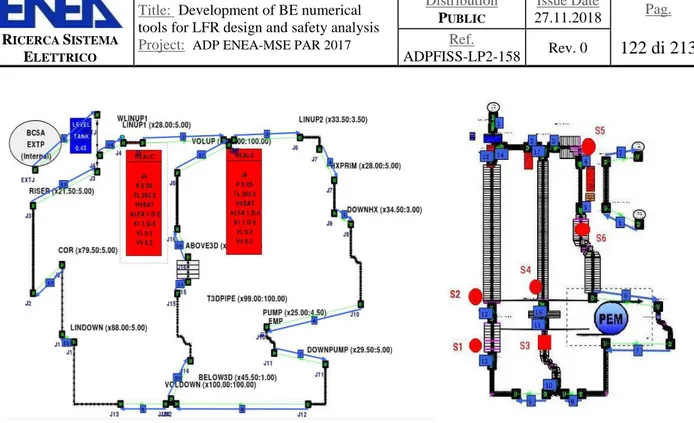
Fig. 4.7 - One-dimensional CATHARE model for the TALL-3D facility (left) and point of interests S1-S2 of the left leg (right), S3-S4 of the central leg and S5-S6 of the right vertical leg. ... 122

Fig. 4.8 - Modelling for TALL-3D. Geometry and dimensions. ... 122

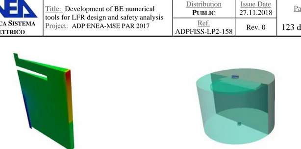
Fig. 4.9 - OpenFoam modelling for TALL-3D. The three-dimensional test section in Open Foam mesh (format in UNIV or MED). ... 123

Fig. 4.10 - FemLCore modeling for TALL-3D. Geometry and dimensions of the three-dimensional test section. ... 123

Fig. 4.11 - TrioCFD modelling for TALL-3D. Geometry of the axial-symmetric and three-dimensional test section. ... 123

Fig. 4.12 - Temperature over the outlet (A) and inlet boundary (B) as function of time during the stabilization step. ... 124

Fig. 4.13 - Initial steady state for turbulent variable for CFD OpenFoam code with the turbulent flow model κ-ω. ... 125

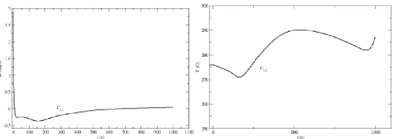
Fig. 4.14 - Cathare stand-alone simulation. Computed mass flow rate 𝒎 (left) and temperature (right) at the points S3-S4 of the central leg as a function of time t. ... 126

Fig. 4.15 - Cathare stand-alone simulation. Computed mass flow rate 𝒎 (left) and temperature (right) at the points S5-S6 of the central leg as a function of time t. ... 126

Fig. 4.16 - Cathare stand-alone simulation. Computed mass flow rate ṁ (left) and temperature (right) at the points S1 of the central leg as a function of time t. ... 126

Fig. 4.17 - Mass flow rate (right) and temperature (left) at reference point S4 (top) and S4 (below) of the central leg for Cathare stand-alone (C) and coupling Cathare-OpenFoam with κ-ω turbulence model. ... 127

Fig. 4.18 - Mass flow rate (right) and temperature (left) at reference point S6 (top) and S5 (below) on the left leg for Cathare stand alone (C) and coupling Cathare-OpenFoam with κ-ω turbulence model. ... 128

(12)

12 di 213

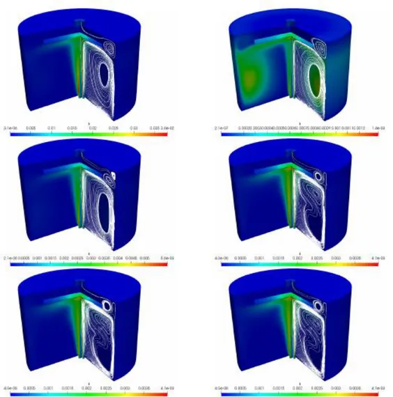
Fig. 4.20 - Turbulent kinetic energy κ and streamline profiles over the three-dimensional test component at t = 0, 4, 20, 80, 180, 580, 1780 and 2780s by using two-equation κ-ω turbulence model in OpenFoam. ... 130 Fig. 4.21 - Mass flow rate (top) and temperature (bottom) at the reference points S3 and S4 for k-ω (kw)

and k-ε (ke) turbulence models. ... 131 Fig. 4.22 - Mass flow rate for OpenFoam (OFS3 ), TrioCFD (TS3), Cathare stand-alone (CS3 ) and

experimental data (ES3) as a function of time. ... 131 Fig. 4.23 - On the left the inlet temperature for OpenFoam (OFS3), TrioCFD (TS3), Cathare

stand-alone (CS3) and experimental data (ES3) as a function of time. On the right the outlet temperature for OpenFoam (OFS4), TrioCFD (TS4), Cathare stand-alone (CS4) and experimental data (ES4). ... 132 Fig. 4.24 - Mass flow rate for OpenFoam (OFS3), TrioCFD (TS3), Cathare stand-alone (CS3) and

experimental data (ES3) as a function of time. ... 132 Fig. 4.25 - Temperature (right) and pressure (left) at the point S3 where boundary conditions are

imposed on a multi-scale interface from OpenFoam (3D) to Cathare (1D) as a function of time after the pump shutdown. ... 132 Fig. 5.1 – Power map of the ALFRED core generated by Serpent (top graph) and power distribution

within three FA at different position in the core. The different spatial gradients are clearly visible. ... 146 Fig. 5.2 – OpenFOAM CFD model of the single FA of ALFRED: the heat source qvol is retrieved from

Serpent, boundary conditions for velocity, temperature and pressure need to be provided, as well as the inter-assembly heat flux qIHX. ... 146 Fig. 5.3 – Serpent radial power map at mid-height in the core at cold condition (T=673K), associated to

keff=1.01027±3pcm (left); Serpent radial power map at hot condition (T=1073K), associated to keff=1.00772±3pcm (right). ... 147 Fig. 5.4 – Comparison of radial (left) and axial (right) power maps calculated with Serpent in cold and

hot conditions. ... 147 Fig. 5.5 – Coupling scheme and definition of simulation phases. ... 148 Fig. 5.6 – Identification of the concentric regions at the same temperature (generated by FRENETIC)

adopted for the Serpent run... 148 Fig. 5.7 – Axial temperature for fuel and coolant in three different FAs of the ALFRED core calculated

with FRENETIC. ... 149 Fig. 5.8 – Radial power distribution for each FA evaluated with FRENETIC (red), as compared with the

Serpent results averaged on the same spatial domain (blue). The identification of the radius along which the comparison is performed also provided. ... 149 Fig. 5.9 – Axial power distribution for three different FAs evaluated with FRENETIC (dotted), as

compared with the Serpent results (dashed), also averaged on the same spatial domain (solid). The localization of the observed FAs is also provided. ... 150 Fig. 5.10 – Pressure drop along the central FA calculated by FRENETIC and OpenFOAM (OF in the

(13)

13 di 213

Fig. 5.13 – Monte Carlo Serpent convergence behavior. The vertical black line indicates the boundary

between inactive and active cycles. ... 152

Fig. 5.14 – Neutron flux spectra computed by Serpent for selected regions of the core. Black dashed lines identify the 5-group energy subdivision originally adopted, while the blue dashed line identifies the additional group added to better account for the reflector spectrum. ... 152

Fig. 5.15 – Axial discretization for the FRENETIC model (black lines) on top of fine Serpent axial discretization for each radial region. ... 153

Fig. 5.16 – FRENETIC model of the ALFRED core. ... 153

Fig. 5.17 – Radial power map (in MW per FA) computed by Serpent (left) and FRENETIC (right) ... 154

Fig. 5.18 – Comparison between the linear power calculated by Serpent and FRENETIC for three selected FAs (left) and radial map of the relative error between the power per FA evaluated by the two codes (right). ... 154

Fig. 5.19 – Radial scheme of the improved FRENETIC model of the ALFRED core. ... 155

Fig. 5.20 – Comparison between the linear power calculated by Serpent and FRENETIC for three selected FAs (left) and radial map of the relative error between the power per FA evaluated by the two codes (right). ... 155

Fig. 5.21 – Linear power calculated by FRENETIC for three selected FAs (left) and axial temperature profiles for fuel and coolant in the same FAs (right) ... 156

Fig. 5.22 – Radial power (left) and peak fuel temperature (right) distribution computed in the coupled FRENETIC simulations. ... 156

Fig. 6.1 – Unstable behavior of Monte Carlo – CFD coupling (EPR case). Evolution of a) volumetric power, b) fuel temperature in the first 4 iterations. ... 171

Fig. 6.2 – The fixed-point coupling algorithm. ... 172

Fig. 6.3 – The stochastic approximation coupling algorithm ... 173

Fig. 6.4 – Radial view (a) and longitudinal view (b) of the SERPENT model of the ALFRED reactor. ... 173

Fig. 6.5 – Power peaking factor of one-fourth of ALFRED reactor core for BOC. ... 174

Fig. 6.6 – a) Geometry and b) mesh of ALFRED one-sixth of FA... 174

Fig. 6.7 – Relative power variation at each iteration for the fixed-point scheme. ... 175

Fig. 6.8 – Temperature profile calculated with the Monte Carlo – CFD coupling scheme. ... 175

Fig. 6.9 – Velocity profile calculated with the Monte Carlo – CFD coupling scheme. ... 176

Fig. 7.1 – Data exchange configuration ... 188

Fig. 7.2 – Coupling tool workflow ... 189

Fig. 7.3 – Geometry of the system ... 190

Fig. 7.4 – Stand-alone and coupled nodalizations ... 190

Fig. 7.5 – Case 1 results ... 191

(14)

14 di 213

Fig. 7.9 – Case 5 results ... 193 Fig. 7.10 – Temperature evolution in the low-pressure tank in case 3 ... 193 Fig. 7.11 – Geometrical features of the LIFUS5/Mod3.3 facility and nodalization scheme ... 194 Fig. 7.12 – SIMMER III nodalization of the LIFUS5/Mod3.3 facility (S1-B tank and ending injection

line part) ... 195 Fig. 7.13 – Initial conditions (from time = 0 to time =1) of the SB1 Tank – Fluids typology (LEFT),

PbLi temperature (CENTER) and Fluids density (RIGHT) ... 195 Fig. 7.14 – Time = 1.03 s (0.03 s after start of injection) - Fluids typology (LEFT), PbLi temperature

(CENTER) and Fluids density (RIGHT) ... 196 Fig. 7.15 – Time = 1.04 s - Fluids typology (LEFT), PbLi temperature (CENTER) and Fluids density

(RIGHT) ... 196 Fig. 7.16 – Time = 1.05 s - Fluids typology (LEFT), PbLi temperature (CENTER) and Fluids density

(RIGHT) ... 197 Fig. 7.17 – Time = 1.06 s - Fluids typology (LEFT), PbLi temperature (CENTER) and Fluids density

(RIGHT) ... 197 Fig. 7.18 – Time = 1.04 s - Fluids typology (LEFT), LiOH volume fraction (CENTER) and Li2O volume

fraction (RIGHT) ... 198 Fig. 7.19 – Time = 1.06 s - Fluids typology (LEFT), LiOH volume fraction (CENTER) and Li2O volume

fraction (RIGHT) ... 198 Fig. 8.1 – Methods (in bracket) and software packages (in grey) for simulating relevant phenomena in

nuclear fuel. ... 208 Fig. 8.2 – Integration of the Thermochimica thermochemistry library into the multiphysics ... 208 Fig. 8.3 – Coupling between the thermo-mechanical fuel code ALCYONE, the inert fission gas model

MARGARET, and the thermo-chemical code ANGE. ... 209 Fig. 8.4 – DSC curve of the system Pb – CeO2: temperature profile and heat flow curve. ... 209 Fig. 8.5 – Sample holder for XRD analysis: CeO2 (left) and Fe2O3 (right). ... 210 Fig. 8.6 – XRD patterns of Ce2O pellet after reactivity experiment with Pb at 550°C (top) and 750°C

(bottom). ... 210 Fig. 8.7 – XRD patterns of La2O3 pellet after reactivity experiment with Pb at 550°C. ... 211

(15)

15 di 213

L

IST OF TABLES

Tab. 1-1 – Collection of the helium solubility in oxide fuel [1.45] ... 30

Tab. 2-1 – CIRCE S100 main parameters ... 48

Tab. 2-2 – TEST IV boundary conditions ... 48

Tab. 2-3 – CIRCE-ICE nodalization scheme: main parameters ... 48

Tab. 3-1 – Dissymmetrical test: sequence of events ... 81

Tab. 3-2 – Seady state conditions ... 81

Tab. 4-1 – Thermocouples and temperature measurement. ... 115

Tab. 4-2 - STH modeling for TALL3D. Basic functions for the interface ICoCo class over the Salome platform. ... 115

Tab. 4-3 - Cathare modeling for TALL-3D. Interface functions for exchange data of the Cathare-Salome platform (ICoCo class). ... 115

Tab. 4-4 - OpenFOAM modeling for TALL-3D. Basic functions for interface construction of the OFclass over the SALOME platform for exchange data. ... 116

Tab. 4-5 - OpenFOAM modeling for TALL-3D. Interface functions of the OpenFOAM- SALOME platform. OpenFOAM solution 𝝓 mapped into MEDField 𝝓. ... 116

Tab. 4-6 - FemLCore modeling for TALL-3D. Basic functions for interface construction of the FEMUS class over the SALOME platform. ... 116

Tab. 4-7 - FemLCore modelling for TALL-3D. Interface functions of the FemLCore-SALOME platform. FemL-Core solution 𝝓 mapped into MEDField 𝝓. ... 117

Tab. 4-8 - TrioCFD modelling for TALL-3D. Basic functions for interface ICoCo class over the SALOME platform for exchange data. ... 117

Tab. 4-9 - TrioCFD modelling for TALL-3D. Interface functions of the TrioCFD-SALOME platform (ICoCo class). TrioCFD solution 𝝓 mapped into MEDField 𝝓. ... 117

Tab. 4-10 - Physical properties used in the modeling of the TALL-3D facility. ... 118

Tab. 4-11 - Initial state condition for the one-dimensional Problem C (cathare). The STH code initial condition satisfies the steady state equation. ... 118

Tab. 5-1 – Upper energy of the 5-group discretization adopted in the generation of cross sections for the Serpent-OpenFOAM/FRENETIC comparison. ... 145

Tab. 5-2 – Resulting energy group boundaries. ... 145

Tab. 5-3 – Temperatures values adopted for the Serpent runs used to evaluate the few-group cross sections. ... 145

Tab. 6-1 – Comparison of some core parameters. ... 169

(16)

16 di 213

Tab. 7-2 – Geometrical features of the LIFUS5/Mod3.3 facility... 186

Tab. 7-3 – Design data of the LIFUS5/Mod3.3 facility ... 186

Tab. 7-4 – Summary of the pressure drop coefficients implemented in the RELAP5 nodalization (LIFUS5/Mod3.3 facility) ... 187

Tab. 7-5 – Initial and boundary conditions for the SIMMER/RELAP5 simulation of LIFUS5 ... 187

Tab. 8.1 - Results of the DSC preliminary investigations ... 207

(17)

17 di 213

L

IST OF ABBREVIATIONS

AdP Accordo di Programma

ALFRED Advanced Lead Fast Reactor European Demonstrator

ATHENA Advanced Thermal Hydraulic Experiment for Nuclear Application BE Best Estimate

BEPU Best Estimate Plus Uncertainty BoP Balance of Plant

BoT Beginning of Transient

CEA Commissariat a l'Energie Atomique et aux Energies Alternatives CFD Computational Fluid Dynamics

CIRCE Circolazione Eutettico

CIRTEN Interuniversity Consortium for Technological Nuclear Research CHEOPEIII Chemistry Operation III Facility

CR Control Rod

DBA Design Base Accident DHR Decay Heat Removal DHRS Decay Heat Removal System DOC Design-Oriented Code DSA Deterministic Safety Analysis

ESFRI European Strategy Forum on Research Infrastructures EoT End of Transient

FA Fuel Assembly

FALCON Fostering ALFRED Construction FPC Fuel Performace Code

FR Fast Reactor

GIORDI Grid to Rod fretting facility HBS High Burnup Structure

HELENA Heavy Liquid Metal Experimental Loop for Advanced Nuclear Applications HLM Heavy Liquid Metal

HX or HEX Heat Exchanger

I&C Instrumentation and Control LBE Lead Bismuth Eutectic LECOR Lead Corrosion Loop

LEADER Lead-cooled Advanced Demonstration Reactor LIFUS5 Lead-Lithium for Fusion Facility (5)

LFR Lead Fast Reactor LM Liquid Metal LMR Liquid Metal Reactor LWR Light Water Reactor MA Minor Actinide

MABB Minor Actinides Bearing Blankets MOX (U-Pu) Mixed Oxide

NACIE Natural Circulation Experiment Loop NPPs Nuclear Power Plants

O&M Operation and Maintenance PAR Piani Annuali di Realizzazione

(18)

18 di 213

PSA Probabilistic Safety Analysis

RACHELE Reactions and Advanced chemistry for Lead RSE Ricerca Sistema Elettrico

RV Reactor Vessel

RVACS Reactor Vessel Air-Cooling System SA Safety Analysis

SET-PLAN Strategic Energy Technology Plan SG Steam Generator

SGTR Steam Generator Tube Rupture SISO Single Input Single Output

SYS System

SYS-TH System- ThermalHydraulics TH Thermal-Hydraulics TKE Turbulent Kinetic Energy TRL Technological Readiness Level TSO Technical Safety Organization ULOF Unprotected Loss of Flow UNIBO Università di Bologna UNIPI Università di Pisa

UNIROMA1 Università di Roma - Sapienza VOC Verification-Oriented Code V&V Verification & Validation AdP Accordo di Programma

ALFRED Advanced Lead Fast Reactor European Demonstrator BE Best Estimate

DSA Deterministic Safety Analysis LFR Lead Fast Reactor

PAR

PSA Probabilistic Safety Analysis RSE Ricerca Sistema Elettrico SA Safety Analysis

(19)

19 di 213

F

OREWORD

The Lead-cooled Fast Reactor (LFR) technology brings about the possibility of fully complying with all the Generation IV requirements. This capability being more and more acknowledged in international fora, the LFR is gathering a continuously increasing interest, with new industrial actors committing on LFR-related initiatives. In this context, the Italian nuclear community evaluates strategic to continue elevating the competences and capabilities, with the perspective of extending the support to the design and safety analysis of future LFR systems. The most appropriate framework for this advancement is the Accordo di Programma (AdP), within which ENEA and CIRTEN (the consortium gathering all Italian universities engaged in nuclear education, training and research) are already cooperating on the LFR technology since 2006, along with national industry as main stakeholder. Within the AdP, the LFR system chosen as reference for all studies and investigations is ALFRED, the Advanced Lead-cooled Fast Reactor European Demonstrator. As a demonstration reactor, indeed, it was reckoned as the system best fitting with the research and development (R&D) nature of the activities performed in the AdP, being demonstration the step that logically follows R&D in the advancement of the LFR technology by readiness levels. Moreover, ALFRED is envisaged as the key facility of a distributed research infrastructure of pan-European interest, open to scientists and technologists for relevant experiments to be performed on a fully LFR-representative and integral environment, with the long-term perspective of supporting to the safe and sustainable operation of future LFRs, thereby fulfilling the general objectives of the AdP itself.

In the wide spectrum of possible activities to support the further development of the LFR technology, and exploiting the specific expertise acquired by the universities in the past years, within the scope of the 2016 Piano Annuale di Realizzazione (PAR) it was decided to focus the cooperative efforts shared between ENEA and CIRTEN towards the development of an best estimate computational tools supporting the various stages of design and safety analyses of LFR systems, so to increase – or help in viewing how to fill the gaps – the modeling capabilities.

(20)

20 di 213

(21)

21 di 213

1 T

HERMO

-M

ECHANICS OF THE FUEL PIN

–

DEVELOPMENT AND ASSESSMENT OF MODELS AND ALGORITHMS DESCRIBING INERT GAS BEHAVIOR FOR USE IN

TRANSURANUS

(22)

22 di 213

(23)

23 di 213

1.1 Background and references

This activity is twofold: first, we present the derivation of two new correlations based on available literature data for helium solubility in oxide nuclear fuel; second, we present a new algorithm for the solution of coupled partial differential equations for inert gas behaviour modelling. Both these contributions are intended for implementation and use in the TRANSURANUS fuel performance code (FPC), for its application to fast reactors.

1.1.1 Helium solubility

The knowledge of helium behaviour in nuclear fuel is of fundamental importance for its safe operation and storage [1.1],[1.2]. This is true irrespectively of the fuel cycle strategy adopted. In fact, both open and closed fuel cycles tend towards operating nuclear fuel to higher burnups (i.e., keeping the fuel in the reactor for a longer time to extract more specific energy from it), thus implying higher accumulation of helium in the fuel rods themselves [1.3]. Moreover, considering open fuel cycles foreseeing the disposal of spent fuel, the helium production rate in the spent nuclear fuel is positively correlated with the burnup at discharge, and the production of helium (by α-decay of minor actinides) progresses during storage of spent fuel [1.4],[1.5]. On the other hand, closed fuel cycles imply the use of fuels with higher concentrations of minor actinides (e.g., minor actinides bearing blankets, MABB), thus being characterized by higher helium production rates during operation [1.4].

Helium is produced in nuclear fuel by ternary fissions, (n,α)-reactions and α-decay [1.6]-[1.8]. After its production, it precipitates into intra- and inter-granular bubbles and can be absorbed/released from/to the nuclear fuel rod free volume [1.9],[1.10]. Helium thus contributes to the fuel swelling (and eventually to the stress in the cladding after mechanical contact is established), to the pressure in the fuel rod free volume, and to the gap conductance (giving feedback to the fuel temperature) [1.11].

Among the several properties governing the behaviour of helium in nuclear fuel, its diffusivity and solubility govern the transport and absorption/release mechanisms [1.12]-[1.14]. Compared to xenon and krypton, helium presents both a higher solubility and a higher diffusivity in oxide nuclear fuel [1.5]-[1.17]. A considerable amount of experiments has been performed with the goal of determining the diffusivity and solubility of helium in nuclear fuel [1.12]-[1.5],[1.18]-[1.27]. In particular, several measurements have been made to determine the helium diffusivity as a function of temperature [1.13]-[1.15],[1.19]-[1.27] and its Henry’s constant as function of temperature [1.12]-[1.15],[1.18]-[1.20],[1.28].

In the light of the profound differences in microstructure of the samples, the correlations for He-UO2 Henry’s constant derived from rough data fitting must be critically analysed. No correlations are currently implemented in the TRANSURANUS code for this parameter, beside its expected modelling importance.

1.1.2 PolyPole-2 algorithm

The first and basic step of fission gas release (FGR) and gaseous swelling is gas atom transport to the grain boundaries. It follows that modelling of this process is a fundamental component of any fission gas behaviour model in a fuel performance code. Intra-granular fission gas transport occurs by thermal and irradiation-enhanced diffusion of single gas atoms, coupled to trapping in and irradiation-induced resolution from intra-granular bubbles. Diffusion of intra-granular bubbles becomes relevant at high temperatures, above ~1800°C [1.29],[1.30]. Thus, modelling the process of gas transport to the grain boundaries calls for the treatment of different concomitant processes, namely, diffusion coupled with trapping and resolution of gas atoms. Extensive literature deals with the evaluation of the parameters characterizing these mechanisms, both experimental and theoretical work, e.g., [1.29],[1.31]-[1.34]. In this activity, we deal with the numerical

(24)

24 di 213

analysis. In fact, the solution of these equations is required in each mesh point of the engineering FPCs. Efficient solutions are thus mandatory to guarantee acceptable overall computational times.

Speight [1.35] proposed a simplified mathematical description of intra-granular fission gas release. He lumped the trapping rate, β (s-1), the re-solution rate, α (s-1), and the diffusion coefficient, D (m2 s-1) into an effective diffusion coefficient, Deff = α / (α + β) D, restating the mathematical problem as purely diffusive, i.e., simplifying the system

in which c1 (at m -3

) is the single-atom gas concentration, m (at m-3) is the concentration of gas trapped in intra-granular bubbles, and yF (at fiss-1 · fiss m-3 s-1) is the production rate of gas atoms, to

where ctot (at m -3

) is the total gas concentration. Such simplification implies the assumption of equilibrium between trapping and re-solution (quasi-stationary approach). The formulation of Speight is universally adopted for models employed in fuel performance codes, e.g., [1.36]-[1.42]. In addition, the assumption of spherical grain geometry [1.10] is applied. The solution of the diffusion equation for constant conditions is well known. Nevertheless, time-varying conditions are involved in realistic problems. Therefore, the solution for time-varying conditions is the issue of interest for applications to fuel performance analysis, which calls for the development of dedicated numerical algorithms. As briefly stated above, given the very high number of calls of each local model (such as the fission gas behaviour model) in a fuel performance code there is a requirement of low computational cost (in addition to the requirement of suitable accuracy for the numerical solution). Clearly, the numerical solution of the diffusion equation in time-varying conditions may be obtained using a spatial discretization method such as a finite difference scheme. However, the high associated computational effort can make a space-discretization based solution impractical for application in fuel performance codes. Several alternative algorithms, which provide approximate solutions for Eq. 1.2 at high speed of computation and can be used in fuel performance codes, have been developed[1.36]-[1.38],[1.43].

We propose a numerical algorithm for the accurate and fast solution of both Eqs. 1.1, 1.2 in time-varying conditions, which we refer to as PolyPole. We verify the algorithms for Eqs. 1.1 with specifically designed numerical experiments.

As demonstrated in [1.44], the solution of this general system of PDEs (Eqs. 1.1) is of high engineering importance, especially related to modelling fission gas behaviour in the high burnup structure (HBS) during reactivity-initiated accidents (RIA).

1.2 Body of the report concerning the ongoing activities

In Sect. 1.2.1, we provide a complete overview of all the experimental results obtained for helium solubility 𝜕𝑐₁ 𝜕𝑡 = 𝐷∇2𝑐1− 𝛽𝑐1+ 𝛼𝑚 + 𝑦𝐹 𝜕𝑚 𝜕𝑡 = +𝛽𝑐1− 𝛼𝑚 (1.1) 𝜕𝑐_𝑡𝑜𝑡 𝜕𝑡 = 𝛼 𝛼 + 𝛽𝐷∇2𝑐𝑡𝑜𝑡+ 𝑦𝐹 (1.2)

(25)

25 di 213

complemented by an uncertainty analysis. These correlations represent a step forward in the development of a helium behaviour physics-based model in TRANURANUS, with respect to the diffusivity correlations derived as part of the POLIMI activities for the PAR 2016.

In Sect. 1.2.2, we describe an algorithm (PolyPole-2) dedicated to the solution of coupled partial differential equations relevant for inert gas behaviour modelling in fuel performance codes. The here presented algorithm is preliminary verified with a random numerical experiment. This algorithm extends the algorithm for the solution of the effective diffusion equation (PolyPole-1) developed as part of the POLIMI activities for the PAR 2015.

1.2.1 Helium solubility

After the verification of the validity of Henry’s law for the He-UO2 system and the classification of the resulting data based on the sample microstructure (not reported here for the sake of brevity, see [1.45]), we derive empirical correlations for Henry’s constant of helium in oxide fuel.

As a starting point, we recall Henry’s law

where kH (at m -3

MPa-1) is Henry’s constant and p (MPa) is the helium pressure. The solubility is thus a function of temperature and pressure. If Henry’s law is valid for the He-fuel system1_{, Henry’s constant is} solely a temperature function.

Following [1.45], we collect in Tab. 1-1 an overview of the available experimental data of solubility. Helium solubility in uranium dioxide have been also extensively studied theoretically by [1.46]-[1.49], but this results are not included in the current analysis. Theoretical results are overall in line with experimental ones[1.45].

Assuming the validity of Eq. 1.3, we need to derive a correlation for Henry’s constant as a function of temperature. The data presented in Tab. 1-1 are reported in Fig. 1.1, divided based on the microstructure of the sample, i.e., powders and single crystals. As expectable, powders show a generally higher apparent Henry’s constant in all the temperature range compared to single crystals, since helium is accumulated in-between different particles. Unfortunately, no data are available for polycrystalline materials (either experimental or lower-length scale simulation results).

Despite the large scatter of the experimental results for the helium solubility in uranium dioxide, the resulting clustering of the data motivated the derivation of two distinct correlations in the form kH = A exp(−B/kT). The best estimate correlation for Henry's constant in the powder samples is

and the best estimate correlation for Henry’s constant in the single crystal samples is

1_{The validity of Henry’s law in the system of interest can be verified with solubility data at different pressures and}

same temperature. The only dataset available with these characteristics is the one by [1.20], reported in Tab. 1-1. At each of three temperatures (1473 K, 1623 K, 1773 K) he performed infusions at three pressures (4.8 MPa, 6.9 MPa, 9.0

𝑐𝑆,He= 𝑘𝐻(𝑇)𝑝 (1.3)

(26)

26 di 213

Summarizing the uncertainty analysis concerning the fit of the solubility correlations, it is important to notice that the functional form used is Log kH = Log A – B/kT Log e. Thus, we have the following confidence intervals at 95% confidence level: Log A (at m-3 MPa-1) = 25.25 (23.91, 26.6) for Eq. 1.4, and 24.61 (23.41, 25.82) for Eq. 1.5; B (eV) = 0.41 (0.06, 0.75) for Eq. 1.4, and 0.65 (0.28, 1.01) for Eq. 1.5; the R2 are respectively 0.83 and 0.83, for Eq. 1.4 and Eq. 1.5. These fitting parameters have been derived applying the LAR (least absolute residuals) method.

Regarding the applicability, the correlation derived fitting the data concerning the powder samples (Eq. 1.4) is usable for the analysis of the helium behaviour in the fuel after the pulverization occurred during accidental temperature transients [1.30],[1.50]. On the other hand, the correlation proposed for Henry's constant in single crystals (Eq. 1.5) is of interest for calculations in meso-scale intra-granular and inter-granular models dealing with single fuel grains.

1.2.2 PolyPole-2 algorithm

In this Section, we present the new numerical algorithm solving Eqs. 1.1 in time-varying conditions, referred to as PolyPole-2 [1.44]. A simplified version of the same algorithm, referred to as PolyPole-1 [1.51], solving Eq. 1.2.

To simplify the notation, it is convenient to re-write Eqs. 1.1 as

in which u = [c1 m] and S = [yF 0] are vectors containing the gas concentrations and the fission source term, respectively. The diffusion D and exchange E operators are defined as

The boundary conditions of Eq. 1.6 are u(r = a, t) = 0 and ∂u/∂r|(r = 0) = 0. The initial condition is u(r, t = 0) = u0(r) = [c0(r) m0(r)].

Under the quasi-stationary approximation [35], the diffusion-exchange operator (D + E) is replaced by Dα/(α + β)∇2_{, S is replaced by yF and u is replaced by c}

tot = c1 + m (i.e., Eq. 1.2).

Here, the objective is to find an approximate solution u* for the case of time-varying (D + E) and S. With the ansatz that the solution can be approximated as

𝑘_𝐻 = 4.1 ∙ 1024_{exp⁡(−0.65/𝑘𝑇)} (1.5) 𝜕 𝜕𝑡𝑢 = (𝐃 + 𝐄)𝑢 + 𝐒 (1.6) 𝐃 = [𝐷∇₀2 0₀] (1.7) 𝐄 = [−𝛽 +𝛼_{+𝛽 −𝛼]} (1.8) 𝑢∗_{(𝑟, 𝑡) ≈ ∑ 𝑧} 𝑛∗(𝑡)𝜓𝑛(𝑟) = ∞ ∑ 𝐏_𝑛𝑧_𝑛(𝑡)𝜓𝑛(𝑟) ∞ (1.9)

(27)

27 di 213

in which zn(t) and 𝜓n(r) are the time coefficients and the spatial modes, respectively, of the solution for constant conditions (exponential in time and cardinal sine in space). The operator Pn embodies the correction for time-varying conditions and is applied to each mode of the solution. The formulation adopted in this work for this operator is made of two distinct polynomials of second order J

This definition of Pn reduces to a single polynomial correction factor for the PolyPole-1 algorithm [1.51]. The problem of finding an approximate solution for time-varying conditions is basically shifted to the problem of finding the coefficients of the polynomials in Pn. To calculate the coefficients pj and qj, 2J equations are needed. This set of equations is obtained by sampling the time-varying operators, D(t), E(t) and S(t), at J uniformly distributed instants along the time-step dt. The sets of sampled values, D[j], E[j] and S[j], contain the information on the variation of the operators along the time step and are used to calculate the corrective polynomials as follows.

The time coefficients z*(t) defined by Eq. 1.9 are assumed to satisfy Eq. 1.6 (here written in vector notation) at the sampling times t[j], ti ≤ t[j] ≤ ti+1

Eq. 1.11 defines a linear system of 2J equations for the polynomial coefficients pj and qj , and is used to determine the polynomial correction operator Pn. The time coefficients of the analytic solution for constant conditions, zn, are calculated using averages along the time step of the sampled values D[j], E[j] and S[j]. The PolyPole-2 (and PolyPole-1, identically) solution is then reconstructed as a linear combination of the spatial with the corrected time coefficients, according to Eq. 1.9. The series is approximated by a finite number of terms (M, number of modes). The value of M is determined based on a D'Alembert-like remainder criterion.

The verification of PolyPole-2 is performed via a random numerical experiment [1.44]. The numerical experiment consists of the application of the PolyPole-2 algorithm to the numerical solution of Eqs. 1.6 for many randomly generated histories. The results from the PolyPole-2 algorithm are compared to the reference solution provided by a finite difference (FD) algorithm (developed as part of previous activities. Details of this method can be found in [1.52]). This algorithm can be applied to obtain a reference solution of Eqs. 1.1 and 1.2 (in principle, up to any tolerance) for piecewise-linear operation histories. The considered histories, both for RIA-like and operational transients, are in terms of temperature and fission rate, from which the time-dependent parameters in the diffusion and exchange operators, D(t) and E(t), and in the source term, S(t), are calculated2.

The figure of merit chosen for this numerical experiment is the fractional intra-granular fission gas release at the end of the considered history, defined as

𝐏_𝑛= [ 1 + ∑ 𝑝𝑗𝑑𝑡𝑗 𝐽 𝑗=1 0 0 1 + ∑ 𝑞𝑗𝑑𝑡𝑗 𝐽 𝑗=1 ] (1.10) 𝜕(𝐏_𝑛𝑧_𝑛) 𝜕𝑡 |𝑡[𝑗]= ⟨𝜓𝑛|𝐃[𝑗] + 𝐄[𝑗]|𝜓𝑛⟩(𝐏𝑛𝑧𝑛) + ⟨𝜓𝑛|𝐒[𝑗]⟩ (1.11)

(28)

28 di 213

where tend (s) is the end time of each history considered.

In order to verify the PolyPole-2 algorithm in fast transient conditions, we consider RIA-like conditions. We considered two sets of representative random histories. The first one, which is referred to as centre, is designed to represent the intra-granular gas diffusion during an RIA transient in the centre of the pellet. The second one, referred to as rim, is designed to be representative of the intra-granular gas behaviour during a RIA transient in the high burnup structure (HBS) at the rim of the pellet (for which a specific formation model has been developed as part of POLIMI activities in previous PARs). These two sets of histories differ in the grain size a, which is assumed as 5.0 μm for the centre and as 150 nm for the rim, respectively. We consider an initial gas concentration corresponding to the gas generated during an irradiation up to 50 GWd tU-1. This initial gas concentration is assumed to be stored in the grains in the centre (70% as single atoms and 30% as atoms in bubbles) [1.39]. In the rim, the initial concentration is set to 1026 at m-3, corresponding to the asymptotic gas concentration achieved in the HBS grains [1.53],[1.54]. The RIA-like random histories have the following characteristics (identical for both centre and rim):

 The peak width, τRIA, is a random variable, sampled uniformly over 20-60 ms.

 The specific energy, ERIA, is a random variable, sampled uniformly over 400-800 J (gUO2) -1

.  The maximum specific power, PRIA (W g

-1

), is calculated as PRIA = 62.5 ERIA/τRIA [55,56].

 The power pulse shape is calculated according to the Nordheim-Fucks model [55,56].

 The initial temperature, T0 (K), is calculated as T0 = 883 (5 10-4 ERIA + 0.7772) (uniform in the range 863-1039 K) [55].

 The maximum temperature, Tmax (K) is calculated as Tmax = 2564 (5 10-4 ERIA + 0.7772) (uniform in the range 2506-3017 K) [55].

 The maximum temperature is reached after 2τRIA, i.e., at the end of the power pulse. The temperature increase in time is calculated as the integral of the power pulse.

 The end time is fixed at 300 ms after the beginning of the RIA-transient.  The final temperature, Tend (K), is calculated as Tend = 1227 (5 10

-4

ERIA + 0.7772) (uniform in the range 1200-1444 K) [55].

 Prior to RIA-transient each history has a plateau of 100 hours at T0, to ensure the establishing of equilibrium between single gas atoms and gas in bubbles.

The results of the RIA-like numerical experiment are presented in Fig. 1.2. Each data point in these figures corresponds to one of the randomly generated operation histories and represents the intra-granular fission gas release (Eq. 1.12) obtained with the PolyPole-2 algorithm versus the reference FD solution. The deviation from the 45° line is a measure of the accuracy of PolyPole-2. Results appear to be distributed between two clusters of data points. The higher intra-granular fission gas release results (5 to 15%, approximately) are the 𝜒 =∫ 𝑦𝐹(𝑡 ′_)d𝑡′ 𝑡𝑒𝑛𝑑 0 − 𝑐1(𝑡𝑒𝑛𝑑) − 𝑚(𝑡𝑒𝑛𝑑) ∫𝑡𝑒𝑛𝑑𝑦𝐹(𝑡′_)d𝑡′ 0 (1.12)

(29)

29 di 213

In Fig. 1.2, we also report the results from the FD solution of Eq. 1.2 for the same input histories. The comparison highlights the effect of the quasi-stationary approximation (implied in Eq. 1.2) for the analysis of fast transients. Results demonstrate that the quasi-stationary approximation is inadequate in describing the fast transients to relatively high temperatures (e.g., RIAs) considered in this study. In particular, the approximation leads to a strong unacceptable under-prediction of the intra-granular fission gas release. Besides accuracy, speed of computation is an essential feature for an algorithm to be effectively employed in a fuel performance code. The computational time (i.e., the time taken for the analysis of a single operation history) for the 2 and FD algorithms are compared in Fig. 1.3. The computational time of PolyPole-2 is approximately two orders of magnitude lower than that of the FD algorithm. Such efficiency of computation, combined with the demonstrated accuracy, makes PolyPole-2 suitable for implementation in TRANSURANUS.

1.3 Role of the activity, general goals and future development

The activity represents an ideal continuation of previous efforts carried out at POLIMI in modelling the impact of inert gas behaviour on the thermo-mechanical performance of oxide nuclear fuels and for the advancement of available numerical tools for the simulation of oxide fuel in LFR conditions [1.57],[1.58]. In this picture, helium solubility (herein treated in terms of its Henry’s constant) plays a fundamental role in determining oxide fuel swelling and fuel rod pressurization, thus affecting its thermo-mechanical behaviour under both normal operation and transient conditions. Moreover, since high burnups are attractive from an economical perspective, modelling the formation of the high burnup structure and its peculiar thermo-mechanical behaviour is of the utter relevance to the safe operation of oxide-fuelled rods in LFR systems. The exposed advancements in the numerical algorithm PolyPole, suited for the efficient solution of the governing equations of inert gas behaviour physics-based models in fuel performance codes, are essential in perspective to improve the numerical capabilities of fuel performance codes. Besides allowing for the treatment of inert gas behaviour models, these advancements pave the way for the treatment of other fundamental meso-scale phenomena (e.g., point defects and thermochemistry).

Future efforts will be devoted to further improvements of the description of helium behaviour. We have now all the instruments (developed among the POLIMI contribution to previous PAR and current PAR 2017) for the definition of a physics-based describing helium behaviour in oxide fuel and for its inclusion in TRANSURANUS. The next steps are going to be the development of the model itself, the implementation of the model in TRANURANUS exploiting the PolyPole algorithms, and the comparison of model results with experimental data. Moreover, the development of a burnup module allowing for accurate, yet fast, prediction of helium production rate is of interest for future activities in different kind of fuels of interest for lead cooled fast reactors (again, in continuity with previous POLIMI activities in PARs).

The overall goal of POLIMI activities within PARs is the set-up and application of an improved LFR-oriented TRANSURANUS version, with focus on the inert gas behaviour physics-based multi-scale modelling approach.

(30)

30 di 213

Reference Sample He infusion

pressure (MPa)

Solubility (at m-3) Temperature (K)

Powders

Belle (1961) UO2 powder

(≈0.16 μm) 0.1 2.13 ∙ 10

22

1073

Hasko and Szwarc (1963)

UO2 powder ₁₁ 9.91 ∙ 1022 ₁₀₇₃

Bostrom (as reported by Rufeh, 1964) UO2 powder (≈0.15 μm) 0.1 0.1 6.59 ∙ 1022 3.08 ∙ 1022 1073 1273

Rufeh et al. (1965) UO_{(≈4 μm)}2 powder 10 5 10 1.81 ∙ 1025 4.52 ∙ 1024 8.72 ∙ 1024 1473 1473 1573

Blanpain et al. (2006) UO_{(≈10 μm)}2 powder 0.2 0.2 0.2 1.26 ∙ 1023 1.14 ∙ 1023 1.07 ∙ 1023 1273 1473 1573 Single crystals

Hasko and Szwarc (1963)

UO2 single crystal ₁₁ 1.65⁡∙ 1022 ₁₀₇₃

Sung (1964) UO_{(≈1 μm)}2 single crystal 4.8 6.9 9.0 4.8 6.9 9.0 4.8 6.9 9.0 1.34⁡∙ 1023 2.61⁡∙ 1023 3.35⁡∙ 1023 1.72⁡∙ 1023 3.13⁡∙ 1023 4.05⁡∙ 1023 2.02⁡∙ 1023 4.05⁡∙ 1023 5.83⁡∙ 1023 1473 1473 1473 1623 1623 1623 1773 1773 1773

Blanpain et al. (2006) UO2 single crystal

(≈10 μm) 0.2 1.07⁡∙ 10

22

1573

Maugeri et al. (2009) UO2 single crystal 100

100 1.38⁡∙ 1023 2.16⁡∙ 1023 1523 1743 Nakajima et al. (2011) UO2 single crystal (≈18 μm) 90 1.03⁡∙ 10 25 1473

Talip et al. (2014) UO2 single crystal 98.7 1.99⁡∙ 10 23

1500

(31)

31 di 213

Fig. 1.1 – Plot of the experimental Henry's constant of helium in oxide fuel classified depending

on the microstructure of the sample (i.e., blue for the powder samples and red for the single

crystal samples). Each cluster is fitted by a distinct correlation (dark red and dark blue) [1.45]

(32)

32 di 213

Fig. 1.2 – Comparison between intra-granular fission gas release calculated by the reference

algorithm for the general PDE system (non-equilibrium) and the PolyPole-2 results – red points

– and the FD results for the quasi-stationary approximation (equilibrium) – black points –. Each

data point corresponds to a calculation with randomly generated RIA conditions. The distance

from the 45° dashed line is a graphical measure of accuracy [1.44]

(33)