Filogeografia comparata di alcuni anfibi italiani: implicazioni per la conservazione

U

NIVERSITÀ DEGLI

S

TUDI DELLA

T

USCIA

D

E

S

E

S

D

R

E

G

R

B

(XVIII C

)

T

D

:

F

C

A

A

I

:

I

C

DOTTORANDO

DR. DANIELE CANESTRELLI

COORDINATORE E TUTOR PROF. GIUSEPPE NASCETTI

A mia moglie Paola e mia figlia Alice, le mie buone notizie ogni mattina, i casi di studio che preferisco per le mie ricerche intorno alla diversità.

I

Premessa 1

1. Introduzione 2

1.1 Oscillazioni climatiche del Quaternario e pattern di diversità

genetica 3

1.2 Conservazione degli anfibi in Italia 6

1.3 Le specie studiate 9

2. Canestrelli D., Zangari F. & G. Nascetti. Genetic evidence for two distinct

species within the italian endemic Salamandrina terdigitata Lacépède, 1788 (amphibia: urodela: salamandridae). Herpetological Journal (in press) 12

2.1 Introduction 13

2.2 Materials and methods 14

2.2.1 Allozymes 14 2.2.2 Mitochondrial DNA 15 2.3 Results 16 2.3.1 Allozymes 16 2.3.2 Mitochondrial DNA 17 2.4 Discussion 18 2.5 Nomenclature designation 20 2.6 Conclusion 21

2.7 Tables and figures 23

3. Nascetti G., Zangari F. & D. Canestrelli. The spectacled salamanders,

Salamandrina terdigitata Lacépède, 1788 and S. perspicillata Savi, 1821: 1)

genetic differentiation and evolutionary history. Rendiconti Lincei - Scienze

Fisiche e Naturali 2005, 16:159-169. 34

3.1 Introduction 35

3.2 Materials and methods 35

3.2.1 Sampling 35 3.2.2 Allozyme analysis 36 3.2.3 mtDNA analysis 36 3.3 Results 37 3.3.1 Allozymes 37 3.3.2 mtDNA 38 3.4 Discussion 39

4. Canestrelli D., Verardi A. & G. Nascetti. Genetic differentiation and

history of populations of the Italian treefrog as revealed by the discrepancy between mitochondrial and nuclear genes. (Submitted) 48

4.1 Introduction 49

4.2 Materials and methods 51

4.2.1 Allozymes 52

4.2.2 mtDNA 52

4.2.3 Estimating FST and gene flow for comparative purposes 53

4.3 Results 54

4.3.1 Allozymes 54

4.3.2 mtDNA 56

4.4 Discussion 58

4.5 Conclusions 62

4.6 Tables and figures 64

5. Canestrelli D., Cimmaruta R., Costantini V. & G. Nascetti. Genetic

diversity and phylogeography of the Apennine yellow-bellied toad Bombina

pachypus (Anura: Discoglossidae), with implications for conservation.

(Submitted) 73

5.1 Introduction 74

5.2 Materials and Methods 77

5.2.1 Sampling 77

5.2.2 DNA extraction, amplification and sequencing 77

5.2.3 mtDNA data analysis 78

5.2.4 Allozyme electrophoresis 80

5.2.5 Allozyme data analysis 81

5.3 Results 82

5.3.1 mtDNA 82

5.3.2 Allozymes 85

5.4 Discussion 88

5.4.1 Genetic diversity and population structure 88

5.4.2 Conservation implications 93

5.5 Tables and figures 96

6. Discussione generale 106

6.1 Filogeografia comparata 106

6.2 Implicazioni per la conservazione 113

Ringraziamenti 115

P

Questa tesi si basa sull’analisi dei pattern di diversità genetica in alcune specie di anfibi italiani. Nel capitolo 1 vengono presentate le tematiche e gli obiettivi generali che hanno ispirato lo studio. Per ognuna delle specie studiate i risultati ottenuti sono stati elaborati, discussi ed inviati a riviste scientifiche peer-reviewed per la valutazione e l’eventuale pubblicazione. Ciascuno dei capitoli da 2 a 5 è in ogni sua parte conforme al manoscritto inviato ad una rivista, ad eccezione della letteratura citata che viene presentata in forma cumulativa nell’ultima sezione della tesi. Infine, nel capitolo 6 viene presentata una discussione generale dei risultati ottenuti ed una analisi della loro rilevanza ai fini degli obiettivi generali dello studio.

1. I

La Filogeografia è la disciplina che si occupa dei principi e dei processi che hanno determinato l’attuale distribuzione geografica delle linee genealogiche dei geni, all’interno delle specie e tra specie strettamente affini (Avise, 1987). Nonostante la sua origine recente, le ricerche svolte in quest’ambito hanno prodotto una letteratura scientifica straordinariamente copiosa (Avise, 2000). L’interesse suscitato da questa disciplina nasce dalla possibilità che essa offre di far luce sui processi storici che hanno concorso a strutturare l’attuale distribuzione geografica della variabilità genetica, ma anche sul possibile ruolo di fattori recenti, di origine antropica, nonché sui processi evolutivi a livello di popolazioni, quali pattern di dispersione, passate frammentazioni e/o fluttuazioni demografiche, ecc. (Bermingham & Moritz, 1998; Avise, 2000; Emerson & Hewitt, 2005). Tra i suoi sviluppi certamente più interessanti vi è la Filogeografia Comparata, ossia lo studio dei pattern di concordanza (e discordanza) filogeografica tra taxa aventi distribuzione geografica sovrapposta. La ricerca di pattern comuni nella distribuzione geografica delle specie, è stata al centro dell’attenzione della scienza sin dalla nascita della Biogeografia come disciplina (Wallace, 1869). L’utilizzo di metodiche di genetica biochimica e molecolare e lo sviluppo di studi di filogeografia comparata sta però dando alla biogeografia nuove spinte, consentendole tra l’altro di indagare questioni eco-evolutive classiche, su scale spaziali e temporali più piccole di quanto non fosse stato possibile in precedenza (Arbogast & Kenagy, 2001; Zink, 2002). Questo approccio sta permettendo infatti di individuare eventi criptici di vicarianza che hanno svolto un ruolo determinante nello struttuare le comunità biotiche, di far luce sul ruolo della geografia nei processi di speciazione, nonchè di studiare l’associazione tra cicli climatici e distribuzione geografica delle specie e della variazione genetica all’interno di esse (Bernatchez & Wilson, 1998; Bermingham & Moritz, 1998; Zink, 2002). Esso si sta inoltre rivelando uno strumento particolarmente utile alla pianificazione delle strategie di conservazione di taxa minacciati dal crescente impatto antropico sugli ecosistemi, perchè in grado di fornire informazioni circa l’esistenza di aree

geografiche evolutivamente divergenti e di hotspot di biodiversità genetica (Moritz & Faith, 1998; Avise, 2004).

Nel presente lavoro viene utilizzato un approccio basato sulla filogeografia comparata, per indagare il ruolo di alcuni importanti processi storico-evolutivi nel determinare i pattern di diversità genetica in taxa della penisola italiana, e per fornire informazioni utili alla pianificazione degli interventi di conservazione della batracofauna. Di seguito i due obiettivi verranno introdotti e presentati separatamente.

1.1 O

Q

PATTERN DI DIVERSITÀ GENETICA

Tra i fattori storici che hanno maggiormente contribuito a strutturare l’attuale distribuzione geografica delle specie e della variazione genetica all’interno di esse, vi sono le oscillazioni climatiche del Quaternario (Webb & Bartlein, 1992). L’entità e le modalità delle modificazioni indotte da tali eventi è assai diversa nelle diverse regioni del pianeta, particolarmente in dipendenza della posizione e distanza rispetto all’equatore e alle masse oceaniche, ed all’orientamento delle principali catene montuose (Hewitt, 2004a & 2004b e riferimenti all’interno). In Europa, durante le fasi pleniglaciali la calotta si estendeva a sud fino al 52° parallelo, gran parte della porzione centrale del continente era occupata da tundra e steppe fredde, ed il generale abbassamento del livello del mare di molte decine di metri determinò un arretramento della linea di costa che in alcuni casi, come in Adriatico, riguardò centinaia di chilometri (Van Andel & Tzedakis, 1996). Evidenze fossili, palinologiche e più recentemente genetiche, indicano che numerose specie animali e vegetali sopravvissero alle avverse condizioni climatiche vigenti durante queste fasi rifugiandosi prevalentemente nelle penisole meridionali iberica, italiana, balcanica e in Caucaso (ad es. Hewitt, 2000; ma vedi anche Stewart & Lister, 2001 and

ripristino di condizioni climatiche più favorevoli, durante le fasi interglaciali, gli habitat settentrionali sarebbero stati ricolonizzati a partire dalle aree di rifugio, con conseguente formazione di zone di contatto secondario e di ibridazione tra linee evolutive differenziatesi appunto in rifugi diversi. Il maggior contributo a tale processo di ricolonizzazione sarebbe venuto dalle popolazioni del rifugio balcanico, mentre per effetto dell’orientamento geografico dell’arco alpino e dei Pirenei, minore sarebbe stato il contributo dalla penisola iberica e soprattutto da quella italiana. Una delle principali implicazioni di questo scenario generale è il pattern così detto di “southern richness, northern purity” (Hewitt, 1996, 1999 & 2000), ossia la maggior variabilità genetica riscontrata in popolazioni meridionali (quelle cioè situate nelle aree ipotizzate di rifugio) rispetto a quelle settentrionali. Tale maggior diversità è stata spesso attribuita alla prolungata stabilità demografica che avrebbe caratterizzato queste popolazioni, rispetto a quelle più settentrionali fondate attraverso un processo (l’espansione verso nord dell’areale) implicante successivi colli di bottiglia (Hewitt, 1996 & 2000; ma vedi Bilton et al., 1998; Austerlitz et al., 2000; Petit et al., 2003). Più di recente, il gran numero di filogeografie publicate su taxa della penisola Iberica ha permesso di accostare a questo scenario classico, che implica l’esistenza nelle penisole meridionali di popolazioni grandi e demograficamente stabili per lunghi periodi (di qui in avanti definito scenario P.D.S.), uno scenario in parte alternativo definito di “refugia-within-refugia” (di qui in avanti R.F.R.; Sanz et al., 2000; Guillame et al., 2000; Gomez & Lunt, 2004). Esso prevede che la maggior diversità all’interno della penisola iberica sia da attribuire ad una significativa strutturazione geografica delle popolazioni imputabile almeno in parte all’esistenza di più aree di rifugio, o di fattori comunque in grado di determinare differenziamento allopatrico all’interno di questa penisola. Questa ipotesi, supportata da un crescente numero di evidenze (Jaarola & Searle, 2004; Vila et al., 2005; per una rassegna v.d. Gomez & Lunt, 2004), ha diverse implicazioni. Anzitutto, per effetto della frammentazione, il processo di perdita di variabilità genetica durante la ricolonizzazione degli habitat settentrionali avrebbe avuto luogo a partire da un subset del pool genico originario, e sarebbe perciò stato più drastico. Inoltre, a questi eventi di micro-allopatria avrebbero potuto seguire fenomeni di contatto secondario, il cui ruolo nella formazione degli attuali pattern di

distribuzione della diversità e dei livelli di variabilità genetica delle popolazioni all’interno della penisola potrebbe essere stato fino ad oggi sottostimato.

Anche per quanto riguarda la penisola italiana, uno scenario di P.D.S. è stato ritenuto un plausibile tratto comune della storia di molti taxa, sia da quegl’autori che ne hanno enfatizzato il ruolo come rifugio glaciale e sorgente per le successive ricolonizzazioni degli habitat settentrionali, sia da coloro i quali ne favoriscono una visione come area ad elevata endemicità ma non come sorgente per le ricolonizzazioni (Hewitt, 1996; Bilton et al., 1998; Petit et al., 2003). La recente letteratura relativa a casi di studio dalla penisola iberica suggerisce tuttavia la possibilità che altri processi evolutivi abbiano contribuito a generare tale pattern. Primo obiettivo dello studio che viene qui proposto è dunque quello di valutare quale sia stato il contributo relativo degli scenari P.D.S. e R.F.R. nel determinare l’attuale distribuzione geografica della variazione genetica in taxa della penisola italiana. A tal fine si è scelto di concentrare l’attenzione sulla fauna anfibia, ed in particolare su tre specie di anfibi endemici italiani: Salamandrina terdigitata, Hyla intermedia, Bombina pachypus. Per ciascuna di esse verranno presentate analisi della struttura genetica delle popolazioni, studiata mediante l’utilizzo di marcatori sia nucleari (allozimi) che mitocondriali. I risultati ottenuti verranno valutati sia separatamente per ciascuna delle specie, che comparandoli tra loro e con altri casi di studio al fine di apprezzarne la generalizzabilità.

Alcuni tratti della biologia degli anfibi li hanno resi ormai da lungo tempo organismi molto apprezzati per studi di genetica delle popolazioni. In particolare, la loro generale tendenza ad una modesta vagilità e spiccata filopatria ne determina una scarsa abilità nell’oltrepassare barriere geografiche costituite da habitat sfavorevoli anche di modesta entità (e.g. Austin et al., 2002). Ne consegue che essi siano organismi ideali per lo studio dell’influenza dei diversi fenomeni storici sui pattern di diversità genetica all’interno e tra le popolazioni. Inoltre, anche in virtù delle caratteristiche poc’anzi ricordate, è lecito supporre che specie con caratteristiche ecologiche diverse potrebbero aver risposto in modi diversi alle medesime vicende

storici su un particolare ambiente e le specie ad esso legate, la scelta di studiare specie tra loro diverse in quanto a scelta dell’habitat (vedi paragrafo 1.3) è sembrata la strategia più appropriata. Considerato che le specie di anfibi qui studiate sono anche le prime in Italia peninsulare per le quali saranno disponibili dati da marcatori sia nucleari che mitocondriali, questa scelta consentirà inoltre di estendere le possibilità di comparazione dei risultati ottenuti ad un maggior numero di casi.

1.2 C

I

Nel contesto della generale crisi della biodiversità, particolare attenzione sta ricevendo da ormai più di quindici anni il Declino Globale degli Anfibi, ossia il crollo demografico e l’estesa perdita di popolazioni che si sta verificando praticamente in tutto il pianeta a carico di questa classe di vertebrati. La World Conservation Union (IUCN) ha recentemente pubblicato il Global Amphibian Assessment, concludendo che almeno il 43% delle 5743 specie note di anfibi ha popolazioni in declino, ed il 32% è minacciata di estinzione. Questa percentuale è assai elevata, soprattutto se confrontata con quella relativa ad uccelli e mammiferi (12% e 23% rispettivamente; IUCN, 2004), due gruppi il cui stato di conservazione è universalmente considerato preoccupante. Un ulteriore elemento di preoccupazione deriva dal fatto che gli anfibi sono considerati ottimi indicatori dello stato di conservazione degli ambienti naturali (Vitt et al., 1990; Blaustein & Wake, 1990; Barinaga, 1990; Blaustein & Wake, 1995; Beebee, 1996; Blaustein & Johnson, 2003), sicché un loro declino a livello globale rappresenta certamente un allarmante segnale circa l’attuale condizione degli ecosistemi (Baringa, 1990; Blaustein & Wake, 1995). Tra le maggiori cause del fenomeno vi sono certamente la distruzione e le gravi alterazioni degli habitat naturali da parte dell’uomo, il recente sviluppo epidemico di alcune infezioni, l’introduzione di fauna alloctona, ecc… (per estese revisioni si vedano ad es. Alford & Richards, 1999 e Gardner, 2001). Tuttavia una cospicua mole di casi di declino si sono verificati all’interno di aree protette o comunque non direttamente interessate da attività umane (ad es. Lips, 1998; Stallard, 2001; Blaustein & Kiesecker, 2002). Ciò, se da un lato ha determinato notevole

preoccupazione per l’impossibilità di indicare cause semplici e dirette del fenomeno, dall’altro ha portato allo sviluppo di una gran quantità di ricerche e all’utilizzo dei più diversi strumenti di indagine attraverso i quali è stato possibile giungere all’individuazione di diverse cause complesse ed interazioni tra fattori (Blaustein & Kiesecker, 2002; Blaustein & Johnson, 2003).

Tra i diversi paesi dell’area paleartica occidentale, l’Italia può essere considerata di gran lunga quello a maggior ricchezza di specie di anfibi, oltre la metà delle quali endemiche (Borkin, 1999). Tuttavia, a causa della scarsità di indagini sulla consistenza delle popolazioni attuali e dell’assenza di una adeguata documentazione storica (Shaffer et al., 1998; Andreone & Luiselli, 2000), quadri organici sulla situazione conservazionistica degli Anfibi italiani sono decisamente scarsi, e si basano per lo più su considerazioni di carattere qualitativo (ad es. Bruno, 1973 e 1983; Andreone & Luiselli, 2000). Inoltre, per quanto riguarda gli studi di monitoraggio svolti su singole popolazioni, particolarmente grave è da ritenersi la carenza di dati relativi a lunghi periodi di tempo. Infatti, come ormai accertato da numerosi autori (ad es. Pechmann et al., 1991; Pechmann & Wilbur, 1994; Skelly et al., 1999; Skelly et al., 2003) studi a breve termine hanno scarsissimo valore a fini conservazionistici, non potendo discriminare tra gli eventi di effettivo declino delle popolazioni e le fluttuazioni demografiche naturali caratterizzanti le sottopopolazioni di un sistema a metapopolazione (Hansky, 1994; Hecnar & M’Closkey, 1996; Marsh, 2001).

Per quanto riguarda le singole specie, il maggior contributo alla conservazione degli anfibi italiani è certamente venuto da studi di genetica delle popolazioni. Basti ricordare la profonda revisione che tali studi hanno determinato nell’assetto tassonomico di quasi tutti i gruppi investigati, con l’individuazione di numerose specie criptiche, molte delle quali endemiche. Ricordiamo in proposito, tra gli altri, il caso della raganella italiana (Nascetti et al., 1995), della rana appenninica (Picariello et al., 1990), della salamandra di Lanza (Nascetti et al., 1988), delle diverse specie appartenenti ai generi Hydromantes (Nascetti et al., 1996) e

Picariello, 2000). Tuttavia, molte specie non sono ancora state studiate e soprattutto, nei soli casi delle due salamandre alpine Salamandra atra e Salamandra lanzai sono attualmente disponibili dati circa la struttura e la variabilità genetica relativamente a marcatori sia nucleari sia mitocondriali (Nascetti et al., 1988; Riberon et al., 2001 & 2002). Quest’ultimo aspetto costituisce per gli anfibi italiani un elemento di grave anomalia nel contesto internazionale degli studi di genetica delle popolazioni e genetica della conservazione. In anni recenti si sono infatti andate accumulando evidenze sempre maggiori del fatto che l’utilizzo di un solo marcatore genetico può facilmente portare a conclusioni parziali od errate, e che per contro il confronto dei risultati ottenuti con marcatori aventi modalità di trasmissione ereditaria ed evoluzione diverse, possa costituire in molti casi l’unico strumento attraverso cui giungere ad una corretta documentazione dello stato delle popolazioni e soprattutto alla comprensione dei fenomeni storici che tale stato hanno maggiormente contribuito a determinare (vedi ad es. Piel & Nutt, 2000; Shaw, 2002).

Da quanto fin qui detto emerge come a tutt’oggi non esista un quadro d’insieme tale da costituire quella base scientifica fondamentale per una corretta pianificazione degli interventi di gestione delle specie e di prioritizzazione conservazionistica delle aree geografiche dove esse insistono.

Come sopra ricordato, gli studi di filogeografia e filogeografia comparata possono fornire informazioni di grande rilievo per la biologia della conservazione, in particolare consentendo l’identificazione di aree geografiche evolutivamente divergenti, su cui basare una zonazione “eco-evolutiva” (da contrapporsi all’attuale “politico-aministrativa”) degli interventi di conservazione, nonché di possibili hotspot di diversità genetica verso cui dirigere prioritariamente tali interventi. Ciò individua il secondo obiettivo del presente lavoro, ossia quello di contribuire alla conservazione degli anfibi italiani fornendo il primo contributo utile proprio all’identificazione di tali aree.

L

Le specie oggetto di questo studio, lo ricordiamo, sono tre: la salamandrina dagli occhiali, la raganella italiana, l’ululone appenninico. Di seguito, ciascuna di esse viene presentata brevemente.

La salamandrina dagli occhiali, Salamandrina terdigitata (Lacépède, 1788), è

una specie endemica italiana, diffusa lungo l’arco appenninico dalla Liguria alla Calabria. Essa è anche l’unica rappresentate del suo genere, che tuttavia doveva avere un tempo una diffusione più ampia come testimoniano reperti fossili trovati in Sardegna e Grecia (Lanza, 1988 e riferimenti all’interno). La distribuzione altitudinale di questa specie è abbastanza ampia, dal livello del mare ad oltre 1300 m s.l.m., sebbene sia più frequente nella fascia compresa tra i 200-900 m s.l.m. (e.g. Lanza, 1983; Mazzotti et al., 1999; Corsetti & Angelini, 2000). L’habitat per l’ovideposizione è costituito prevalentemente da torrenti e ruscelli poco profondi e a corso lento, ma non di rado vengono utilizzati i più diversi tipi di ambienti umidi, quali piccoli fossi, pozze effimere, fontanili.

Per quanto riguarda l’inquadramento conservazionistico, la salamandrina dagli occhiali è citata negli Allegati II e IV della Direttiva Habitat (Direttiva 92/43/CEE) ed è inserita in Appendice II della Convenzione di Berna. Essa è inoltre protetta in Italia da leggi a carattere regionale. Tra le molteplici cause di preoccupazione conservazionistica vanno certamente annoverate la frammentazione degli habitat, nonchè l’inquinamento e le alterazioni strutturali dei siti riproduttivi (regimentazionedelle acque, captazione, ...) e delle aree ad essi associati, ad es. mediante esbosco (ad es. Corsetti & Angelini, 2000).

La raganella italiana, Hyla intermedia (Boulenger, 1882), è una specie

endemica dell’Italia e della Sicilia, fino a pochi anni fa attribuita alla specie H. arborea e rivalutata quale buona specie in seguito a ricerche di genetica biochimica (Nascetti et al., 1995). La raganella italiana è un anfibio che nei periodi di attività mostra abitudini spiccatamente arboricole. Attiva principalmente nelle prime ore notturne,

oltre che in pozze di acqua sulfurea (Cucchiara et al., 1996). Per quanto riguarda la distribuzione altitudinale la raganella italiana mostra una spiccata preferenza per le aree di pianura sia costiere che interne. Da quanto riportato negli atlanti erpetologici regionali sembra che l’80-90% delle popolazioni siano situate a quote inferiori ai 400 m s.l.m. (v.d. ad es. Venchi, 2000; Mazzotti et al., 1999; Gasc et al., 1997), sebbene soprattutto nelle porzione meridionale dell'areale esistano segnalazioni di piccole popolazioni situate al di sopra dei 1000 m s.l.m. (c.a. 1500 m s.l.m. presso i Monti della Laga, Ri).

Inserita in Appendice II della Convenzione di Berna (sotto Hyla arborea) e protetta in Italia da leggi regionali, mancano a tutt’oggi studi organici circa lo stato di conservazione di questa specie. Tuttavia è noto che nel corso dell'ultimo secolo essa è scomparsa da estese porzioni dell'areale. Basti citare il caso della Pianura Padana e dell’Agro Pontino, aree che fino circa a metà del secolo scorso la specie popolava con continuità e con popolazioni straordinariamente consistenti, e dove oggi essa risulta invece ampiamente frammentata. Tra le principali cause di minaccia vanno certamente ricordate la distruzione degli habitat riproduttivi, come le così dette zone umide minori, l’inquinamento e la frammentazione di quelli ancora esistenti, l’introduzione di fauna alloctona (soprattutto ittica) e la diffusione di pratiche agricole monocolturali (per più estese discussioni in proposito si vedano Canestrelli, 2002 e Scoccianti, 2001).

L’ululone appenninico, Bombina pachypus (Bonaparte, 1838), è un anfibio

anuro endemico dell’ Italia peninsulare, presente lungo tutto l’arco appenninico dalla Liguria alla punta della Calabria (Lanza, 1983). La sua presenza in Sicilia, pur segnalata per il settore nord-orientale (Bruno, 1970), attende ulteriori conferme. Specie prevalentemente diurna, i siti di riproduzione sono costituiti per lo più da pozze temporanee di piccole dimensioni, poco profonde e soleggiate. Dal punto di vista altitudinale, l’ululone appenninico predilige quote comprese tra 200 e 800 metri s.l.m. (Caputo et al., 1985; Doria & Salvidio 1994; Mazzotti et al., 1999; Sarrocco & Bologna, 2000), anche se occasionalmente lo si può ritrovare fino a 1800 m s.l.m., o al livello del mare (Lanza, 1983; Mazzotti et al., 1999; Sarrocco & Bologna, 2000). Complessivamente dunque, sia dal punto di vista latitudinale sia altitudinale, la

distribuzione geografica di questa specie risulta ampiamente sovrapposta a quella della salamandrina dagli occhiali.

La specie (sotto B. variegata, della quale era fino a poco tempo fa considerata sottospecie) è inserita negli Allegati II e IV della Direttiva Habitat (Direttiva 92/43/CEE) ed è citata in Appendice II della Convenzione di Berna. Essa è inoltre protetta in Italia su base regionale. L’areale di distribuzione della Bombina pachypus risulta fortemente frammentato ed è stato più volte suggerito che diverse popolazioni stanno subendo declino (vedi ad es. Sarrocco & Bologna, 2000; Caputo et al., 1985; Doria & Salvidio, 1994 e riferimenti all’interno). Inoltre diversi autori hanno sottolineato come le popolazioni esistenti siano spesso costituite da un numero esiguo di individui (ad es. Sarrocco & Bologna, 2000). Come per le specie precedenti, tra le cause di minaccia sono certamente da annoverare la distruzione degli habitat riproduttivi e la frammentazione di quelli ancora esistenti, anche a seguito dei cambiamenti nelle tecniche agricolturali. Inoltre per questa specie è stato segnalato il rinvenimento in popolazioni dell’ Appennino settentrionale di individui affetti da Batrachochytrium dendrobatidis (Stagni et al., 2002), un fungo patogeno che ha causato gravi fenomeni di declino in popolazioni di diverse specie di Anfibi da molte parti del pianeta (Daszak, & Hyatt, 2003).

2. G

Salamandrina terdigitata

L

,

1788 (

:

:

).

DANIELE CANESTRELLI, FRANCESCA ZANGARI & GIUSEPPE NASCETTI.

A

Genetic variation in 12 populations of the Italian endemic spectacled salamander, Salamandrina terdigitata (Lacépède, 1788) was investigated through the analysis of 29 allozyme loci and partial sequences of two mitochondrial genes (cytochrome b, 629 bp and 12s rRNA, 444 bp). Both nuclear and mitochondrial markers fully agreed in identifying two well-differentiated population groups, one ranging from Tusco-Emilian Apennine to southern Latium, the other comprising populations from central Campania to Calabria. At the nuclear level, nine diagnostic and four highly differentiated loci led to an average genetic distance of DNEI= 0.47 between both

groups, while within them DNEI ranged from 0.00 to 0.05. At the mitochondrial

level two alternatively fixed haplogroups were found, with an average Kimura-2-parameter sequence divergence of 17% and 8% at the cytochrome b and 12s rRNA genes respectively. The observed genetic structure and the comparison between the levels of divergence recorded with respect to those reported for other salamanders, strongly suggest that two distinct species were so far included within Salamandrina terdigitata. The names Salamandrina perspicillata (Savi, 1821) and S. terdigitata are here proposed for the species from central and southern Italy respectively.

KEYWORDS:Salamandrina terdigitata, Salamandrina perspicillata, spectacled salamander, allozymes, mitochondrial genes, cytochrome b, 12s rRNA, molecular taxonomy.

2.1 I

Since their emergence, biochemical and molecular techniques have allowed the study of the genetic structure of populations, providing evidence for the existence of cryptic biodiversity that was previously unsuspected. For amphibians, which are generally conservative in their morphological evolution (Cherty et al., 1978; Hass et al., 1995; Richards & Moore, 1996), the routine use of these tools has led to the identification of an astonishing number of morphologically “cryptic” species (e.g. Duellman, 1993; Nascetti et al., 1996; Hanken, 1999; Frost, 2002), even in the well-studied European batrachofauna, as recently reviewed by Veith (1996) and Borkin (1999). In fact, the number of amphibian species recognized for the European area has almost doubled during the last four decades (Mertens & Wermuth, 1960; Frost, 2002), but it should be borne in mind that several species have not yet been investigated. Among these, Salamandrina terdigitata constitutes an interesting case study. Many aspects of its natural history are well known, it is of particular concern to Italian zoologists because it is the only Italian endemic terrestrial vertebrate genus (Lanza, 1988), and is protected by international and regional laws (it is listed in the Annexes II and IV of the EU Council Directive for the Conservation of Natural Habitats and of Wild Fauna and Flora). In spite of this, no studies have investigated its geographic variation and genetic population structure to date. This paper is therefore aimed at filling this gap.

The spectacled salamander, Salamandrina terdigitata, is a stream-breeding species endemic of peninsular Italy, mainly distributed on the western side of the Apennine chain from 200m to 900m a.s.l. (Lanza, 1983a; Mazzotti et al., 1999; Corsetti & Angelini, 2000, see Figure 1). It is the only known representative of a genus which, according to the morphological and molecular analysis done by Titus & Larson (1995), is an ancient lineage that separated from other newt lineages very shortly after the split between newts and true salamanders. Fossil records revealed that its distribution was once wider than now, comprising at least Sardinia and

structure and history (e.g. Piel & Nutt, 2000; Shaw, 2002), we here provide data on the genetic population structure of the spectacled salamander assessed by means of allozyme electrophoresis (i.e. a set of nuclear markers) and partial sequences of two mitochondrial genes, cytochrome b and 12s rRNA. Finally, the taxonomic implications of our results will be also discussed.

2.2 M

We collected 149 specimens of Salamandrina terdigitata from 12 populations covering almost the entire species range (Fig.1). The geographical origin of the samples studied and sample sizes are presented in Table 1. Each specimen was anaesthetized in the field with 3-aminobenzoic acid ethyl ester (MS222) following the protocol of Heyer et al. (1994) and tail-clipped (about 2 cm) before being released in the same place. Tail samples were transported to the laboratory in liquid nitrogen containers and stored at –80 °C until further analyses. In order to adjust technical procedures and score liver-active enzymes, five specimens from each sampling site were euthanasized with an excess of MS222, then samples of skeletal muscle and liver were obtained and stored at –80 °C.

2.2.1 ALLOZYMES

Tissues from each specimen were crushed in 0.1 ml of distilled water and adsorbed onto chromatography paper labels. Horizontal electrophoresis was carried out onto 10% starch gels. We studied electrophoretically 20 enzymes encoded by 29 presumptive loci (see Table 2 for description of systems and electrophoretic conditions). Isozymes were numbered in order of decreasing mobility from the most anodal one (Ldh-1 and Ldh-2 correspond to Ldh-A and Ldh-B respectively). Alleles at each locus were designated by their mobility (in mm, standardized conditions) relative to the most common one (100) in the reference population (Taverna, Calabria).

Allele frequencies and estimates of genetic variability (mean observed and expected heterozygosity, percentage of polymorphic loci, and average number of

alleles per locus) were calculated for each population using the software BIOSYS-2 (Swofford & Selander, 1999). Exact significance tests for Hardy-Weinberg equilibrium (HW) were conducted for each locus and sample, then the Bonferroni correction for multiple tests was applied (Rice, 1989).

Genetic distances between populations were calculated with Nei’s (1972) standard genetic distance matrix, which was then used to build an UPGMA phenogram. 1000 bootstrap pseudoreplicates over loci were run to test the reliability of the UPGMA phenogram with the BOOTDIST option in BIOSYS-2. The consensus UPGMA was then obtained using the subroutines NEIGHBOR and CONSENSE in the software PHYLIP 3.5c (Felsenstein, 1993). The cophenetic correlation coefficient, which measures the correlation between distance values calculated during tree building and the observed distance, was also computed. In addition, a hierarchical analysis of molecular variance (AMOVA; Excoffier et al., 1992) was carried out in order to partition total genetic variance into covariance components due to differences within populations, among populations within groups and between groups, using ARLEQUIN 2.000 (Schneider et al., 1999).

2.2.2 MITOCHONDRIAL DNA

Total genome DNA was extracted from frozen tissues following standard phenol/chloroform extraction protocol (Sambrook et al., 1989). We amplified partial sequences of two mitochondrial genes: the cytochrome b and the ribosomal 12s rRNA (12s) via polymerase chain reaction (PCR). For both fragments PCRs were carried out in a final volume of 50 µl containing: 1 µl of genomic DNA, 30 mM KCl, 10 mM Tris HCl pH 8.3, 2.5 mM MgCl2, 0.2 µM of each primer, 0.2 mM of

each dNTP, and 2.5 units of Taq polymerase. PCR cycles for cytochrome b consisted of: 5 minutes of denaturation at 95°C, followed by 40 cycles including denaturation at 93°C for one minute, annealing at 45°C for 45 seconds and extension at 72°C for one minute and 30 seconds, followed by a final extension of 10 minutes at 72°C. PCR cycles for 12s were the same except for the annealing step (50°C for 45

Ethidium Bromide for the staining under UV light. The purified PCR products were double-sequenced using the same PCR primers on an ABI3730 XL automatic DNA sequencer with the standard protocol of the BigDye Terminator v3.1 Cycle Sequencing Kit.

The sequencing chromatograms were analyzed with the program CHROMAS ver. 2.23 (Technelysium Pty Ltd, Australia). Alignments were produced with the software CLUSTALX 1.81 (Thompson et al, 1997). All haplotypes found were deposited in Genbank (Accession Numbers AY695901- AY695907).

We calculated the number of substitutions and genetic distances between haplotypes according to Kimura-2-parameter model (K2P; Kimura, 1980) as implemented in the software MEGA 2.1 (Kumar et al., 2001). This widely-used model (K2P) was chosen because to compare our results with previous studies. Phylogenetic analyses were performed using Maximum Parsimony (MP) and Neighbor Joining (NJ) methods as implemented in PAUP* 4.0b10 (Swofford, 2003). Bootstrap resampling was performed on 1000 pseudoreplicates. Unweighted MP trees were obtained using the exhaustive search. Salamandra lanzai was used as outgroup (GenBank Accession Number AF356699; Riberon et al., 2002).

2.3 R

2.3.1 ALLOZYMES

Thirteen out of twenty-nine loci analyzed (G3pdh, Ldh2, Mdh1, Icdh1, 6Pgdh, G6pdh, Sod1, Aat2, Ck, Adk, PepB2, PepD1, and Pgm1) were monomorphic in all populations surveyed. Allele frequencies at the sixteen polymorphic loci are presented in Table 3. None of the tests for HW equilibrium was significant after Bonferroni correction. Based on allele frequencies at polymorphic loci, the samples can be grouped into two well-differentiated groups, one comprising populations from central Italy (samples 1 to 6), and the other including those from southern Italy (samples 7 to 12). This subdivision is reflected by the two main clusters in the UPGMA phenogram showed in Figure 2 (cophenetic correlation coefficient CCC = 0.995). Nine loci (Mdhp1, Mdhp2, Gapdh, Aat1, Alat, PepB1, PepD2, Tpi, Pgm2)

were fully diagnostic between both groups of populations, while at the other four loci (Ldh1, Icdh2, Mpi, Gpi) distinct alleles were found at moderate to high frequencies in only one of these groups (see Table3). Pairwise values of Nei’s (1972) genetic distances are presented in Table 4. Genetic distances between groups ranged from DNEI=0.41 to DNEI=0.52, with an average value of DNEI=0.47 (standard

deviation -SD- = 0.03), whereas within each of the two groups it varied from DNEI=0.00 to DNEI=0.05, with an average value of DNEI=0.02 (SD = 0.02). Within

the southern group, populations 11 and 12 (Calabria) were the most differentiated, with high bootstrap support (88%) in the UPGMA analysis and presenting an average genetic distance of DNEI=0.03 (SD = 0.01) with respect to the other

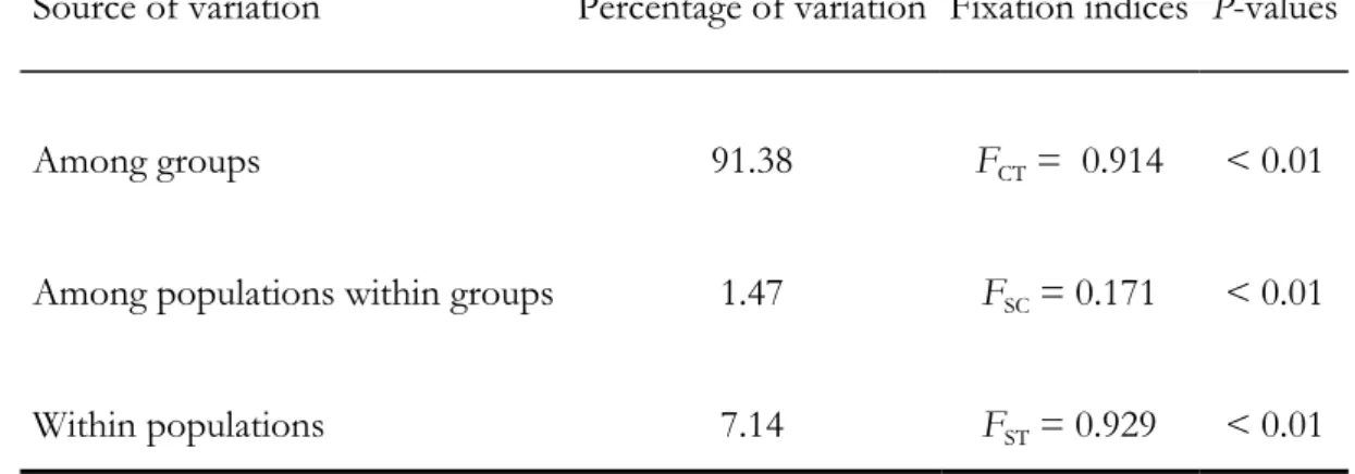
southern samples. When populations were grouped into the two main groups identified by the UPGMA analysis, the results of the AMOVA analysis (Table 5) indicated that up to 91 % of the total genetic variability found in our dataset can be attributed to differences among groups.

Estimates of genetic diversity are presented in Table 3. Expected heterozygosity varied from 0.00 to 0.08, with the highest values in populations from the central group (populations 1, 5 and 6). Within the southern group, the population from Amalfi completely lacks genetic diversity, and that from Serino was polymorphic at only one locus (Ldh1), with HE = 0.01. Other measures of genetic

variability (observed heterozygosity, percentage of polymorphic loci and average number of alleles per locus) exhibited the same geographical pattern as HE.

2.3.2 MITOCHONDRIAL DNA

The amplified fragments of the cytochrome b gene yielded unambiguous sequences of 629 bp without indels, while 12s sequences varied in length from 436 to 444 bp.

For cytochrome b, five distinct haplotypes were defined by 95 variable positions (79 at third positions, 11 at first and five at second, including nine aminoacid replacements). The NJ analysis (Figure 3) identified two

well-steps in length, consistency index CI = 1.00, retention index RI = 1.00, homoplasy index HI = 0.00). All southern specimens (samples 7 to 12) shared a single haplotype (s1), which was never found in samples from central Italy (samples 1 to 6). In the latter, four haplotypes (c1-c4) were found to differ in at most two nucleotide substitutions. Haplotypes c3 and c4 were both observed only once in the population from Percile, whereas c2 was found in a single specimen from Bagno di Romagna. All other specimens from the central-Italy population group shared the haplotype c1.

Nucleotide variation was less pronounced at the 12s fragment: only two distinct haplotypes with a K2P genetic distance of 0.08 were detected, one in each group of samples.

2.4 D

We observed a particularly significant pattern of genetic differentiation among the studied populations. In fact, both mitochondrial and nuclear markers fully coincide in delimiting two well-defined clusters of closely related samples, one comprising the samples from Tusco-Emilian Apennine to southern Latium (samples 1-6), and the other including those from central Campania to southern Calabria (samples 7-12). As evidenced by the AMOVA analysis, most of the genetic variation observed at allozymes (91 %) can be attributed to differences between both groups, with only a small amount of the total variation attributable to within-group variation.

Levels of genetic divergence were found to be unexpectedly high considering the restricted distribution of this species (it is an Apennine endemism [e.g. Lanza, 1983a]), as well as its apparent morphological homogeneity. The pattern of genetic divergence observed with allozymes (nine diagnostic loci, and four other that were highly differentiated at allele frequencies, leading to an average DNEI = 0.47)

resembles that found between several congeneric species of salamanders. For instance, Nascetti et al. (1996) found values of DNEI ranging from 0.33 to 0.40

strinatii), whereas among species of Hydromantes from eastern Sardinia (H. flavus, H. imperialis and H. supramontis) the same authors (see also Lanza et al., 1995) found DNEI values ranging from 0.47 to 0.48. Similar values have been also reported for

some species of the genus Triturus (e.g. Macgregor et al., 1990). At the mitochondrial level, the values of K2P divergence observed within S. terdigitata (17 % for cytochrome b and 8 % for 12s) exceed those reported in the literature for other congeneric species of salamanders. For instance, Riberon et al. (2001) reported K2P values for the widely studied cytochrome b gene ranging from 10.6% to 12.8 % between Salamandra atra and S. salamandra. These values are close to those found by García-París et al. (2003) between S. salamandra and S. algira (10.4%) and by Caccone et al. (1997) between Euproctus platycephalus and E. montanus (11.7 %). Several other case studies of congeneric species of amphibians presenting comparable degrees of divergence at cytochrome b sequences have been reviewed by Johns & Avise (1998). These authors evidenced how in the majority of pairwise congeneric species comparisons, K2P divergence ranges from 10 to 20 % in amphibians. But to our knowledge, no case study has been described to date showing two conspecific lineages of salamander diverging at cytochrome b gene sequences to as great an extent as those we found within Salamandrina terdigitata.

Following the above arguments, the two well-differentiated evolutionary lineages found within the spectacled salamander might represent two distinct taxa, for which we propose the rank of species. As will be discussed below, we suggest the name Salamandrina perspicillata for the northern species, while S. terdigitata should be retained for the southern one.

A substantial genetic homogeneity was found within both species, notwithstanding the fact that within S. terdigitata the populations from Calabria are distinctive according to allozymes. For several populations of Salamandrina, levels of genetic diversity resemble the average values reported by Nevo & Beiles (1991) for representatives of the family Salamandridae (HE = 0.058; P = 24.0%). However, the

from a combination of both factors. At this time we are unable to distinguish between these possible causes, even if the poor conservation status and fragmentation of the habitats in the Italian peninsula are likely to have played some role.

2.5 N

As mentioned by Lanza (1988), the spectacled salamander was originally described by Lacépède (1788) with the name Salamandra ter-digitata on the basis of a single specimen collected by M. le Comte de Milly from Vesuvius. Fifteen years later, the species was also described (under the name Salamandra tridactyla) by Daudin (1803), who based his description on a specimen collected by De Nesle in the same locality. Later, another description was published by Savi (1821), who described the new species Salamandra perspicillata from cool and shady sites of Tuscan Apennine and particularly Mugello. He believed that he had found a new salamander species, because Lacépède’s salamander was described as having four toes on the hind feet, but only three toes on the front feet. Later studies indicated that the two salamanders belonged to the same species, the original description by Lacépède being based on a poorly preserved specimen. Following the principle of priority of the International Code of Zoological Nomenclature, the species was given the name chosen by Lacépède, changed into terdigitata by removing the hyphen. Finally, Fitzinger (1826) proposed that the species belonged to a distinct monotypic genus, which he named Salamandrina. Other names have subsequently been proposed for the species, but they were all later synonymised (e.g. Salamandra imperati Costa, 1828; Salamandra savi Cuvier, 1829).

According to the principle of chronological priority and the geographic origin of our samples, we suggest that the name Salamandrina perspicillata (Savi, 1821) be used for the species from central Italy, while the name Salamandrina terdigitata (Lacépède, 1788) be retained for the southern species. However this new nomenclatural arrangement will need to be further discussed, depending on the identity of the type specimens being confirmed. The analyses of type specimens will

follow the completion of morphological analyses, now in progress, to identify potential morphological differences of diagnostic value between the two species. At present the two species can be diagnosed based on their genetic divergence, as assessed at both mtDNA sequence (Cytochrome-b and 12s rRNA genes) and diagnostic allozyme loci (Mdhp1, Mdhp2, Gapdh, Aat1, Alat, PepB1, PepD2, Tpi, Pgm2). Moreover, the geographic origin of specimens is also of diagnostic value, although the species assignment of populations from the central portion of the Volturno river drainage basin still needs to be assessed (see Figure 1).

2.6 C

The main outcome of this study has been the recognition of two distinct species within the Italian endemic Salamandrina terdigitata. Future efforts will be focused on two main fields: morphological variation, and genetic analyses of intermediate populations.

In many amphibians, previously undescribed morphological variation has often been assessed after species recognition in genetic studies (e.g. Nascetti et al., 1988; Nascetti et al., 1995). Since no studies to date have investigated morphological variation within the spectacled salamander, future studies will attempt to identify potential differences of diagnostic value between S. terdigitata and S. perspicillata at the level of chromatic, morphological and osteological characters. However, preliminary observations suggest that some chromatic differences do exist between the species. The ventral surface of the tail exhibits a bright red in S. terdigitata, whereas it looks reddish to brownish-orange in S. perspicillata. In addition, the demarcation between the dorsal and ventral coloration of the tail is sharper in S. terdigitata than in S. perspicillata.

With respect to genetic studies, further sampling will be focused on presumed or potential contact zones, such as mid-altitude areas of the Volturno

case, to delimitate it and to address what kind of genetic and ecological interactions are occurring between both species in this area.

Finally, the split of the former S. terdigitata into two distinct species with restricted geographical distributions, strongly suggests the necessity of a careful evaluation of their conservation status, as well as the importance that they be included in the main international lists of threatened species, such as the IUCN Red List.

2.7 T

Table 1. Geographic origin and sample size (n) of the 12 populations of S. terdigitata studied.

Region n Sample code Locality Altitude

(m a.s.l.) Allozymes mtDNA

1 Bagno di Romagna 460 Emilia-Romagna 20 3

2 Barbarano Romano 340 Latium 9 4

3 Tolfa 480 Latium 7 5

4 Percile 575 Latium 11 5

5 Bassiano 560 Latium 12 6

6 M.te San Biagio 140 Latium 10 4

7 Serino 630 Campania 18 4

8 Amalfi 15 Campania 12 5

9 S. Severino Lucano 880 Basilicata 14 5

10 Viggianello 560 Basilicata 8 4

11 Taverna 670 Calabria 18 8

Table 2. Enzymes studied in S. terdigitata, their commission number (EC), encoding loci, buffer systems and tissues used in electrophoresis (M = skeletal muscle, L = liver).

Enzyme EC Encoding loci Buffer systems Tissue Glycerol-3-phosphate dehydrogenase 1.1.1.8 G3pdh 5 M Lactate dehydrogenase 1.1.1.27 Ldh-1 4 M Ldh-2 4 M Malate dehydrogenase 1.1.1.37 Mdh-1 5 M

Malate dehydrogenase (NADP+_{) 1.1.1.40 Mdhp-1 2,5 M, L}

Mdhp-2 2,5 M, L

Isocitrate dehydrogenase 1.1.1.42 Icdh-1 6 M

Icdh-2 6 M 6-Phosphogluconate dehydrogenase 1.1.1.44 6Pgdh 5 M Glucose-6-phosphate dehydrogenase 1.1.1.49 G6pdh 1 M Glyceraldehyde-3-phosfate dehydrogenase _1.2.1.12 Gapdh 6 M

Superoxide dismutase 1.15.1.1 Sod-1 3 M

Aspartate transaminase 2.6.1.1 Aat-1 5 L, M

Aat-2 5 L, M

Alanine transaminase 2.6.1.2 Alat 2, 7 L

Creatine kinase 2.7.3.2 Ck 2 L

Adenylate kinase 2.7.4.3 Adk 2 L

L-LeucylGlycylGlycine Peptidase 3.4.13 Pep-B1 7 M, L

Pep-B2 7 M, L

Table 2. (continue)

Pep-D2 2, 7 M, L

Carbonic anhydrase 4.2.1.1 Ca-2 3 M

Triose-phosphate isomerase 5.3.1.1 Tpi 2 L

Mannose phosphate isomerase 5.3.1.8 Mpi 3 M

Glucose phosphate isomerase 5.3.1.9 Gpi 3 M

Phosphoglucomutase 5.4.2.2 Pgm-1 4 M

Pgm-2 4 M

Pgm-3 4 M

Pgm-4 4 M

Buffer systems: 1) Discontinous Tris/Citrate pH 8.7 (Poulik, 1957); 2) Continous Tris/Citrate pH 8.0 (Selander et al., 1971); 3) Tris/Versene/Borate pH 8.0 (Brewer & Sing, 1970); 4) Tris/Maleate pH 7.4 (Brewer & Sing, 1970); 5) Phosfate-Cytrate pH 6.3 (Harris, 1966); 6) Histidine/Citrate pH 7 (Cheliak & Pitel, 1984); 7) Lithium-borate pH 8.3 (Soltis et al., 1983).

Table 3. Allele frequencies and estimates of genetic variability at 16 polymorphic loci for the twelve populations of Salamandrina terdigitata sampled. Populations are numbered as in Table 1. Population 1 2 3 4 5 6 7 8 9 10 11 12 Locus Ldh1 100 0.79 0.83 0.90 0.95 0.93 1.00 0.17 - 0.23 0.06 0.97 0.80 110 0.21 0.17 0.10 0.05 0.07 - - - - 112 - - - 0.83 1.00 0.77 0.94 0.03 0.20 Mdhp1 100 - - - 1.00 1.00 1.00 1.00 1.00 1.00 102 0.17 - - - - - 104 0.83 1.00 1.00 1.00 0.36 0.25 - - - - 108 - - - - 0.64 0.75 - - - - - - Mdhp2 100 - - - 1.00 1.00 1.00 1.00 1.00 1.00 112 1.00 1.00 1.00 1.00 1.00 1.00 - - - - Icdh2 88 1.00 1.00 1.00 1.00 1.00 1.00 - - 0.27 0.42 0.50 0.44 100 - - - 1.00 1.00 0.73 0.58 0.50 0.56 Gapdh 100 - - - 1.00 1.00 1.00 1.00 1.00 1.00 110 1.00 1.00 1.00 1.00 1.00 1.00 - - - -

Table 3. (continue) Aat1 100 - - - 1.00 1.00 1.00 1.00 1.00 1.00 120 0.50 1.00 0.88 1.00 1.00 0.25 - - - - 130 0.28 - 0.12 - - 0.75 - - - - - - 140 0.22 - - - - - Alat 70 0.10 - - - - - 80 0.90 1.00 1.00 1.00 1.00 1.00 - - - - 100 - - - 1.00 1.00 1.00 1.00 1.00 1.00 PepB1 95 1.00 1.00 1.00 1.00 1.00 1.00 - - - - 100 - - - 1.00 1.00 1.00 1.00 1.00 1.00 PepD2 100 - - - 1.00 1.00 0.94 0.88 1.00 1.00 105 0.17 - - 0.06 - - - - - 110 0.83 1.00 0.88 0.56 0.50 0.85 - - - - 115 - - - 0.06 0.12 - - 120 - - 0.12 0.38 0.50 0.15 - - - - - - Ca2 90 - - - 0.19 0.25 0.40 100 1.00 1.00 1.00 1.00 1.00 1.00 1.00 1.00 1.00 0.81 0.75 0.60 Tpi 100 - - - 1.00 1.00 1.00 1.00 1.00 1.00 105 1.00 1.00 1.00 1.00 1.00 1.00 - - - - Mpi 95 0.70 0.69 0.60 0.70 0.83 0.85 - - - -

Table 3. (continue) Gpi 95 0.15 0.44 0.30 0.23 0.29 0.25 - - - - - - 100 0.85 0.56 0.70 0.77 0.71 0.75 1.00 1.00 1.00 1.00 1.00 1.00 Pgm2 100 - - - 1.00 1.00 1.00 1.00 1.00 1.00 103 - - - - 0.07 0.30 - - - - - - 106 1.00 1.00 1.00 1.00 0.93 0.70 - - - - - - Pgm3 90 - - - - - - - 0.03 - 100 1.00 1.00 1.00 1.00 1.00 1.00 1.00 1.00 1.00 1.00 0.94 1.00 108 - - - - - - - 0.03 - Pgm4 90 - - - - - - - 0.04 - 100 1.00 1.00 1.00 1.00 1.00 1.00 1.00 1.00 0.92 1.00 0.89 0.95 106 - - - - - 0.08 - 0.07 0.05 P95 24.1 10.3 17.2 10.3 20.7 20.7 3.4 0.0 13.8 13.8 13.8 17.2 A 1.3 1.1 1.2 1.2 1.2 1.2 1.0 1.0 1.1 1.1 1.2 1.2 (0.1) (0.1) (0.1) (0.1) (0.1) (0.1) (0.0) (0.0) (0.1) (0.1) (0.1) (0.1) HE 0.08 0.04 0.06 0.05 0.07 0.08 0.01 0.00 0.04 0.04 0.04 0.06 (0.03) (0.02) (0.03) (0.03) (0.03) (0.03) (0.01) (0.00) (0.02) (0.02) (0.02) (0.03) HO 0.09 0.04 0.06 0.03 0.07 0.07 0.01 0.00 0.04 0.03 0.03 0.06 (0.03) (0.02) (0.03) (0.02) (0.03) (0.03) (0.01) (0.00) (0.02) (0.02) (0.01) (0.03) P95 = percentage of polymorphic loci with the most common allele not exceeding 95%. A

= mean number of alleles per locus. HE = average expected heterozygosity assuming

Hardy-Weinberg equilibrium. HO = average observed heterozygosity. Standard errors in

Table 4. Pairwise values of standard Nei’s (1972) genetic distances among the 12 populations of Salamandrina terdigitata sampled. Populations are numbered as in Table 1.

Population 1 2 3 4 5 6 7 8 9 10 11 12 1 - 2 0.01 - 3 0.01 0.00 - 4 0.01 0.01 0.00 - 5 0.03 0.03 0.02 0.02 - 6 0.03 0.05 0.04 0.05 0.03 - 7 0.47 0.51 0.49 0.49 0.49 0.49 - 8 0.48 0.52 0.50 0.51 0.51 0.50 0.00 - 9 0.45 0.48 0.46 0.46 0.47 0.46 0.00 0.01 - 10 0.45 0.48 0.47 0.47 0.47 0.47 0.01 0.01 0.00 - 11 0.41 0.45 0.43 0.43 0.43 0.42 0.04 0.05 0.02 0.03 - 12 0.42 0.46 0.44 0.44 0.44 0.43 0.03 0.04 0.02 0.02 0.00 -

Table 5. AMOVA results for S. terdigitata data as obtained using ARLEQUIN 2.000

(Schneider et al.. 1999). Groups were defined as the two main clusters identified by the UPGMA cluster analysis (Figure 2).

Source of variation Percentage of variation Fixation indices P-values

Among groups 91.38 FCT = 0.914 < 0.01

Among populations within groups 1.47 FSC = 0.171 < 0.01

Figure 1. Species range (A) and geographic location of the 12 populations sampled of S.

Figure 2. UPGMA tree showing genetic relationships among the 12 populations of S.

terdigitata, based on Nei’s (1972) standard genetic distance values. Bootstrap values > 70% over 1000 pseudoreplicates are indicated. Populations are numbered as in Table 1.

Figure 3. Neighbour Joining tree based on Kimura-2-parameter divergence values (K2P) for cytochrome b haplotypes (629bp) observed within S. terdigitata. Bootstrap values over 1000 pseudoreplicates are shown at the nodes when exceeding 70% .

3. T

,

Salamandrina terdigitata

L

, 1788

S. perspicillata

S

, 1821: 1)

.

GIUSEPPE NASCETTI, FRANCESCA ZANGARI & DANIELE CANESTRELLI.

A

Recent genetic investigations revealed the existence of two distinct species within the former Salamandrina terdigitata, once considered the only representative of its Italian endemic genus. The pattern of genetic differentiation between Salamandrina terdigitata and S. perspicillata, as previously assessed with both allozyme and mitochondrial markers, was further analyzed and compared with that observed among other congeneric species of European salamanders. Partial sequences of cytochrome b and 12S rRNA mtDNA genes were therefore obtained from four European species of the genus Salamandra. Genetic differentiation was particularly high within Salamandrina at mitochondrial level, with values of K2P divergence (17 % and 6 % for cytochrome b and 12s respectively) exceeding those of many other species of related salamander. The presence of a Salamandrina Miocenic fossil record from Sardinia suggests that the common ancestor of S. terdigitata and S. perspicillata could have been a Corsica-Sardinian element. The distribution and the depth of genetic divergence between the two species could be the result of a vicariance event, through the separation of the Calabro-Peloritan massif from Sardinia (7.8-8.6 Myr ago), followed by a subsequent dispersal from Corsica-Sardinia plate toward the continent during late Messinian (about 5-6 Myr ago), or through one of the Plio-Pleistocenic land-bridges between the Corsica-Sardinia plate and the Tuscan Archipelago.

KEYWORDS: spectacled salamanders, Salamandrina terdigitata, Salamandrina

3.1 I

The Italian endemic Salamandrina FITZINGER,1826 (Urodela: Salamandridae) is the only European endemic terrestrial vertebrate genus (Lanza, 1988). According to the morphological and molecular analysis of Titus & Larson (1995), it is considered an ancient lineage that separated from the other newt lineages around the time of the split between the remaining newts and the true salamanders. Fossil records have revealed that its distribution was once wider, comprising at least Sardinia and Greece (e.g. Vanni & Nistri, 1997).

Salamandrina terdigitata LACÉPÈDE, 1788 has long been considered the only living species of the genus. However, recent genetic studies based on both nuclear and mitochondrial markers (Canestrelli et al., in press), revealed the existence of two well differentiated species within the spectacled salamander. Consequently, populations spanning from Liguria to central Campania have been recognized under the name Salamandrina perspicillata SAVI, 1821, whereas the name Salamandrina terdigitata LACÉPÈDE, 1788 was retained for populations from central Campania to the tip of Calabria. The Volturno river drainage basin (Figure 1) was suggested as the area of possible close contiguity between the two species, although their reciprocal distribution (i.e., if allopatric or parapatric) has not yet been clarified.

In this paper, the pattern of genetic divergence between Salamandrina terdigitata and S. perspicillata is further investigated and compared with that observed among other species of European salamanders. Moreover, hypotheses about the historical events which led to the observed pattern of divergence are discussed.

3.2 M

individual was carried to the laboratory, euthanasized with an excess of 3-aminobenzoic acid ethyl ester (MS222) and then samples of skeletal muscle and liver were removed and stored at –80 °C. These specimens were used to adjust experimental protocols and to score liver-active enzymes. The second sampling session was carried out in the same collection sites, but this time each specimen was anesthetized in the field with MS222 following suggestions given by Heyer et al. (1994) and tail-clipped (2-3 cm) before being released in the same place. Tissue samples were carried to the laboratory in liquid nitrogen containers and stored at -80 °C to await further analysis. Geographic origin of samples studied and sample size are given in Table 1.

3.2.2 ALLOZYME ANALYSIS

Standard horizontal starch gel electrophoresis was used to study genetic variation at level of 20 enzymes encoded by 29 presumptive loci. The following loci were studied: G3pdh, Ldh-1, Ldh-2, Mdh-1, Mdhp-1, Mdhp-2, Icdh-1, Icdh-2, 6Pgdh, G6pdh, Gapdh, Sod-1, Aat-1, Aat-2, Alat, Ck, Adk, Pep-1, PepB-2, PepD-1, PepD-2, Ca-2, Tpi, Mpi, Gpi, Pgm-1, Pgm-Ca-2, Pgm-3, Pgm-4. Details of the electrophoretic techniques implemented can be found in Canestrelli et al. (in press).

Genetic distances among population were estimated using Nei’s (1972) standard genetic distance (DNEI) and Rogers (1972) distance (DR), using the software

BIOSYS-2 (Swofford & Selander, 1999). DNEI was then used to build an UPGMA

phenogram, whose reliability was assessed with 1000 bootstrap replicates over loci. 3.2.3 MTDNA ANALYSIS

As described in Canestrelli et al. (in press), genomic DNA was extracted following standard phenol:chloroform protocol (Sambrook et al., 1989). Partial sequences of the mitochondrial cytochrome b gene (629bp) and 5’-end of the 12S rRNA (436 to 444 bp) were obtained by means of PCR-amplification using primers’ pairs MVZ15-MVZ16 and 12SZL-12SFH respectively (Moritz et al., 1992; Goebel et al., 1999), followed by double-sequencing on a ABI3730 XL automatic DNA sequencer. In this study, the 3’-end of the 12S rRNA fragment was also sequenced in order to obtain the almost complete sequence of this mtDNA region for all the

previously sequenced specimens. With this aim, a PCR-amplification was carried out using the primers’ pair 12SAL-tRNAvalH (Palumbi et al., 1991; Goebel et al., 1999) and PCR protocol as for the 5’-end fragment. Since the two 12S rRNA fragments were partially overlapping, they were here joined and analyzed as a single sequence (836-844 bp).

For comparative purposes, partial sequences of the same two mitochondrial genes were also obtained from alcohol preserved specimens of the following species (Nascetti legit; two specimens each): Salamandra salamandra from Volpaia (Italy), S. corsica from Vizzavona (Corsica), S. atra from Asiago (Italy) and S. lanzai from Pian del Re (Italy). Sequence for S. luschani was obtained from GenBank (Accession Numbers: AF154053).

The sequences were aligned using CLUSTALX 1.81 (Thompson et al., 1997). All the haplotypes found were deposited in Genbank (Accession Numbers: AY695901- AY695907, AY928613-AY928621).

Number of substitutions and genetic distances between haplotypes according to Kimura-2-parameters model (K2P; Kimura, 1980) were assessed using the software MEGA 2.1 (Kumar et al., 2001). This software was also used to implement the Tajima’s relative rate test (1993), under the null hypothesis of constant substitution rate among sequences. Ambystoma mexicanum was used as outgroup (Accession Number: NC005797).

3.3 R

3.3.1 ALLOZYMES

As shown in Table 2, genetic distances between the two species ranged from DNEI=0.41 to DNEI=0.52 and from DR=0.37 to DR=0.42, with average values of

DNEI=0.47 (0.03 SD) and DR=0.39 (0.01 SD). Within S. perspicillata, DNEI varies

ranging from 0.00 to 0.05 (mean: 0.02 [0.01 SD]) and DR from 0.01 and 0.06 (mean:

0.04 [0.02 SD]).

This pattern is reflected in the UPGMA analysis (Figure 2), where populations of each species clustered together achieving 100% of bootstrap support. 3.3.2 MTDNA

For the spectacled salamanders, partial sequences of 629 bp and 836-844 bp were obtained for cytochrome b and 12S rRNA respectively.

At the cytochrome b fragment, all S. terdigitata specimens shared a single haplotype (s1), that was never found within S. perspicillata samples. In these latter samples, four haplotypes (c1-c4) were found differing at most in two nucleotide substitutions. However, all but three specimens shared the haplotype c1 (haplotypes c3 and c4 were both observed only once in the sample 4, whereas the haplotype c2 was found in one specimen from sample 1). Within Salamandrina, cytochrome b haplotypes were defined by 95 variable positions (79 at the third position, 11 at the first and 5 at the second, with a comprehensive number of 9 aminoacid replacements), and lead to an average genetic distance between the two species of K2P = 0.17 (0.02 SD).

Not surprisingly, genetic divergence between the two species was less pronounced at the 12S rDNA gene. In fact, only two distinct haplotypes were found, alternatively fixed within the two species, differing at level of 45 nucleotide substitution and 5 indels (4 of 1 bp and one of 6 bp in length), with a genetic distance of K2P = 0.06.

Pairwise genetic divergence among the five European species of the genus Salamandra, based on partial sequences of cytochrome b (486 bp) and 12S rRNA (824-837 bp) is shown in Table 3. Within this group of species, ranges of K2P divergence were 0.06-0.22 and 0.03-0.09 for cytochrome b and 12S respectively, with the most differentiated species being S. luschani. This latter species showed an average K2P divergence of 0.20 (0.02 SE) and 0.08 (0.01 SE) at cytochrome b and 12S respectively, compared with the other Salamandra species.

The null hypothesis of constant substitution rate, as assessed by the Tajima’s relative rate test (1993), couldn’t be rejected for any of the 42 tests performed (all P > 0.01).

Assuming 12 Myr of divergence between S. luschani and the other Salamandra species (according to Weisrock et al., 2001), the divergence rate for the mtDNA genes studied here could be estimated at 1.67% and 0.67 % per million years for cytochrome b and 12S respectively.

3.4 D

The recent finding of two well differentiated species within the former Salamandrina terdigitata was a really unexpected result (Canestrelli et al., in press), especially when considering its limited geographic range (restricted to the Apennine chain [e.g. Lanza, 1983a]) as well as the apparent lack of chromatic or morphological variation (with the exception of few chromatic variant described at local level [reviewed by Lanza & Canestrelli, 2002]).

Levels of differentiation found at allozymes between Salamandrina terdigitata and S. perspicillata (DNEI = 0.47, DR=0.39), resemble that found between several

other congeneric species of salamander. For instance, among three Hydromantes species from mainland Italy, Nascetti et al. (1996) found values of DNEI ranging from

0.33 to 0.40, whereas among three Hydromantes species from eastern Sardinia the same authors (see also Lanza et al., 1995) reported values of DNEI ranging from 0.47

to 0.48. Within the genus Triturus (Macgregor et al., 1990), similar values were found between the species pair T. carnifex - T. cristatus (DNEI =0.38), T. carnifex – T. pygmaeus

(DNEI =0.58), T. vulgaris meridionalis – T. pygmaeus (DNEI =0.52) and between T.

pygmaeus and T. marmoratus (DNEI =0.19) which have only recently been recognized

as distinct species (Garcia-Paris et al., 2001).

exceed those achieved by many other species of related salamander. For instance, in the majority of pairwise comparisons among European species of the genus Salamandra (see Table 3), we found values of K2P lower (in same case the half) than that found within Salamandrina. For comparative purpose, we have also recalculated values of K2P for sequences of cytochrome b gene from Pleurodeles and related genera, from recently published data (Veith et al., 2004). As shown in Table 4, K2P genetic divergence between Salamandrina terdigitata and S. perspicillata (17%) results much higher than that found within the genus Pleurodeles and, astonishingly, equals or resembles that found between distinct genera (but “naïve” speculations about taxonomic implications of this observation should be avoided).

The lack of fossil records within the present range of the genus Salamandrina and the lack of a clear geographic barrier to dispersal in the putative area of close contiguity between S. terdigitata and S. perspicillata, permit us neither to unambiguously indicate an historical event nor to directly calibrate molecular clocks, in an attempt to explain the observed pattern and depth of genetic divergence between the two species. Therefore, both tempo and mode of divergence between them have to be estimated indirectly.

By applying to allozymes data a divergence rate of to 0.07 DNEI / Myr,

estimated for plethodontid salamanders (Maxson & Maxson, 1979), the time of divergence between S. terdigitata and S. perspicillata was estimated at 6.71 (±0.43) Myr ago. For mitochondrial sequences, the divergence rates of 1.67% and 0.67% per million year for cytochrome b and 12S respectively, lead to a split-time estimate of 8.96-10.18 Myr ago. Although estimates based on allozymes and mtDNA data don’t overlap, and regardless of the vagaries of molecular clocks (e.g. Ayala, 1997), the depth of genetic differentiation between S. terdigitata and S. perspicillata suggests that their divergence began in the upper Miocene (11-5 Myr ago).

The presence of a Salamandrina Miocenic fossil record from Sardinia suggests that the common ancestor of S. terdigitata and S. perspicillata could have been a Corsica-Sardinian element. Following this argument, and considering the depth of genetic differentiation found between the two species, the most probable paleogeographic event leading to their divergence could have been the separation of