© 2012 ACEEE
Spiking Neural Networks as Analog Dynamical
Systems: Basic Paradigm and Simple Applications
Mario Salerno, Gianluca Susi, Andrea D’Annessa, Alessandro Cristini, and Yari Sanfelice. Institute of Electronics, Rome University at Tor Vergata
E-mail: [email protected]
Abstract — A class of fully asynchronous Spiking Neural Networks is proposed, in which the latency time is the basic effect for the spike generation. On the basis of the classical neuron theory, all the parameters of the systems are defined and a very simple and effective analog simulator is developed. T he p roposed simulator is then a pp lied to elementary exa mp les in wh ich some p rop erties a nd in terestin g applications are discussed.
Index Terms — Neuron, Spiking Neural Network (SNN), Latency, Event-Driven, Plasticity, Threshold, Neuromorphic, Neuronal Group Selection.
I. INTRODUCTION
Spikin g Neural Networ ks (SNN) r epresen t a ver y simple class of simulated neuromorphic systems in which the neural activity consists of spiking events generated by firing neurons [1], [2], [3], [4]. A basic problem to realize realistic SNN concerns the apparently random times of arrival of the synaptic signals [5], [6], [7]. Many methods have been proposed in the technical literature in order to properly desynchronizing the spike sequences; some of these consider transit delay times along axons or synapses [8], [9]. A different approach introduces the spike latency as a neuron property depending on the inner dynamics [10]. Thus, the firing effect is not instantaneous, as it occurs after a proper delay time which is different in various cases. These kinds of neural networks generate apparently random spikes sequences as a number of desynchonizing effects that introduce continuous delay times in the spike generation. In this work, we will suppose this kind of desynchronization as the most effective for SNN simulation. Spike latency appears as intrinsic continuous time delay. Therefore, very short sampling times should be used to carry out accurate simulations. However, as sampling times grow down, simulation processes become more time consuming, and only short spike sequences can be emulated. The use of the event-driven approach can overcome this difficulty, since continuous time delays can be used and the simulation can easily proceed to large sequence of spikes [11],[12].
The class of dynamical neural networks represents an innovative simulation paradigm, which is not a digital system, since time is considered as a continuous variable. This property presents a number of advantages. It is quite easy to simulate very large networks, with simple and fast simulation approach [13]. On the other hand, it is possible
to pr opose very simple logical circuits, wh ich can represent useful examples of applications of the method. The paper is organized as follows: description of some basic properties of the neuron, such as threshold and latency; simulation of the simplified model and the network structure on the basis of the previous analysis; fin ally, discussion of some examples of effective applications of the proposed approach.
II. ASYNCHRONOUSSPIKINGNEURAL NETWORKS
Many properties of neural networks can be derived from the classical Hodgkin-Huxley Model, which represents a quite complete representation of the real case [14], [15]. In this model, a neuron is characterized by proper differential equations describing the behaviour of the membrane potential Vm. Starting from the resting value Vrest , the membrane potential can vary when external excitations are received. For a significant accumulation of excitations, the neuron can cross a threshold, called Firing Threshold (TF), so that an output spike can be generated. However, the output spike is not produced immediately, but after a proper delay time called latency. Thus, the latency is the delay time between exceeding the membrane potential TF and the actual spike generation.
This phenomenon is affected by the amplitude and width of the input stimuli and thus rich dynamics of latency can be observed, making it very interesting for the global network evolution.
The latency concept depends on the definition of the threshold level. The neuron behaviour is very sensitive with respect to small variations of the excitation current [16]. Nevertheless, in the present work, an appreciable maximum value of latency will be accepted. This value was determined by simulation and applied to establish a reference threshold point [13]. When the membrane potential becomes greater than the threshold, the latency appears as a function of Vm Th e laten cy times make th e n etwor k spikes desynchronized, in function of the dynamics of the whole network. As shown in the technical literature, some other solution s can be con sider ed to accoun tin g for desynchronization effects, as, for instance, the finite time spike transmission on the synapses [8], [9], [10].
A simple neural network model will be considered in this paper, in which latency times represent the basic effect to characterize the whole net dynamics.
To this purpose, significant latency properties have been an alysed usin g th e NEURON Simulation 17
© 2012 ACEEE
Environment, a tool for quick development of realistic models for single neurons, on the basis of Hodgkin-Huxley equations [17].
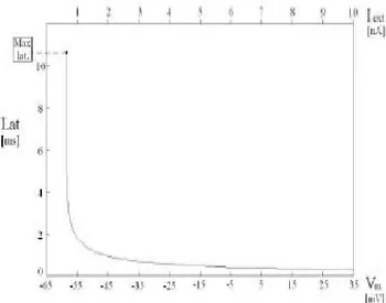
Simulating a set of examples, the latency can be determined as a function of the pulse amplitude, or else of the membrane potential Vm . The latency behaviour is shown in Fig. 1, in which it appears decreasing, with an almost hyperbolic shape. These results will be used to introduce the simplified model, in the next section. Some other significant effects can easily be included in the model, as the subthreshold decay and the refractory period [10] . The consideration of these effects can be significan t in the evolution of th e wh ole n etwork.
Figure 1. Latency as a function of the membrane potential (or else of the current amplitude Iext , equivalently)
III. SIMPLIFIED NEURON MODELIN VIEWOF NEURAL NETWORK
SIMULATION
In or der to in tr oduce th e networ k simulator in wh ich th e laten cy effect is pr esent, th e n eur on is modelled as a system characterized by a real nonnegative in n er state S. Th is state S is modified addin g to it the input signals Pi (called burning signals), coming from the synaptic inputs. They consist of the product of the presynaptic weights (depending on the preceding firing neurons) and the postsynaptic weights, different for each burning neuron and for each input point [13]. Defining th e normalized thr eshold S0 ( > 1) , two
different working modes are possible for each neuron: a) S < S0 , for the neuron in the passive mode;
b) S > S0 , for the neuron in the active mode.
In the passive mode, a neuron is a simple accumulator, as in the Integrate and Fire approach. Some more significant effects can be considered in this case, as the subthreshold decay, by which the state S is not constant with time, but goes to zero in a linear way. Thus, the expression S = Sa – ld is used, in which Sa is the previous state, is the time interval and ld is the decay constant.
In the active mode, in order to introduce the latency
effect, a real positive time-to-fire tf , is considered. It represents the time interval in which an active neuron still remains active, before the firing event. After the time tf , the firing event occurs (Fig. 2) .
Figure 2. Proposed model for the neuron
Th e fir in g even t is con sider ed in stan tan eous an d consists in the following steps:
a) generation of the output signal Pr , called presynaptic weight, which is transmitted, through the output synapses, to the receiving neurons, said the burning neurons ; b) reset of the inner state S to 0 , so that the neuron comes back to its passive mode.
In addition , in active mode, a biun ivocal correspondence between the inner state S and tf holds, called the firing equation . In the model, a simple choice of the normalized firing equation is the following one:
tf = 1/ (S - 1) , for S > S0 .
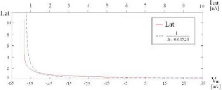
The time tf is a measure of the latency, as it represents the time interval in which the neuron remains in the active state. If S0 = 1 + d (with d > 0), the maximum value of time-to-fire is equal to 1 / d . The above equation is a simplified model of the behaviour shown in Fig. 1. Indeed, as the latency is a func-tion of the membrane potential, time-to-fire depends from the state S, with a similar shape, like a rectangular hyperbola. The simulated and the firing equation behaviours are compared in Fig. 3.
The following rules are then applied for the active neurons.
a) If appropriate inputs are applied, the neuron can enter in its active mode, with a pr oper state SA an d a corresponding time-to-fire tfA = 1/ (SA - 1) .
b) According to the biunivocal firing equation, as the time increases of tx ( < tfA) , the time-to-fire decreases to the value tfB = tfA – tx and the corresponding inner state SA increases to the new value SB = 1 + 1/ tfB.
c) If, after the time interval tx , a new input is received, th e n ew in n er state SB must be con sider ed. As a consequence, the effect of the new input pulse becomes less relevant for greater values of tx .(namely for greater values of SB ).
© 2012 ACEEE
Figure 3. Comparison between the latency behaviour and that of the denormalized firing equation. The two behaviours are
similar to rectangular hyperbola
The proposed model is similar to the original integrateand-fir e model, except for th e in tr oduction of a modulated delay for each firing event. This delay time strictly depends from the inner dynamics of the neuron. Time-to-fire an d firing equation ar e basic con cepts to make asyn ch r on ous th e wh ole n eur al network. Indeed, if no firing equation is introduced, timeto-fire is always equal to zero and any firing event is produced exactly when the state S becomes greater than S0 . Thus, the network activity is not time modulated and
the firing events are produced at the same time. On the other hand, if neuron activity is described on the basis of continuous differential equations, the simulation will be very complex and always based on discrete integration times. The introduction of the continuous time-to-fire makes the evolution asynchronous and dependent on the way by which each neuron has reached its active mode.
In th e classical n eur omor ph ic models, n eur al networks are composed by excitatory and inhibitory neurons. The consideration of these two kinds of neurons is important since all the quantities involved in the pr ocess ar e always positive, in pr esen ce of on ly excitatory firing events. The inhibitory firing neurons generate negative presynaptic weights Pr , and the inner states S of the related burning neurons can become lower. For an y bur ning neur on in th e active mode, since different values of the state S correspond to different tf , time-to-fire will decrease for excitatory, and increase for inhibitory events. In some particular case, it is also possible that some neuron modifies its state from active to passive mode, without any firing process, in the case of proper inner dynamics and proper inhibitory burning event. In conclusion, in presence of both excitatory and inhibitory burning events, the following rules must be considered.
a. Passive Burning. A passive neur on still remains passive after the burning event, i.e. its inner state is always less than the threshold.
b. Passive to Active Burning. A passive neuron becomes active after the burning event, i.e. its inner state becomes greater than the threshold, and the proper the time-to-fire can be evaluated. This is possible only in the case of excitatory firing neurons.
c. Active Burning. An active neuron affected by the burning event, still remains active, while the inner state
can be increased or decreased and the time-to-fire is properly modified.
d. Active to Passive Burning. An active neuron comes back to the passive mode without firing. This is only possible in the case of inhibitory firing neurons. The inner state decreases and becomes less than the threshold. The related time-to-fire is cancelled.
The simulation program for continuous-time spiking neural networks is realized by the event driven method, in which time is a continuous quantity computed in the process. The program consists of the following steps: 1. Define the network topology, namely the burning neurons connected to each firing neuron and the related values of the postsynaptic weights.
2. Define the presynaptic weight for each excitatory and inhibitory neuron.
3. Choose the initial values for the inner states of the neurons.
4. If all the states are less than the threshold S0 no active neurons are present. Thus the activity is not possible for all the network.
5. If this is not the case, evaluate the time-to-fire for all the active neurons. Apply the following cyclic simulation procedure:
5a. Find the neuron N0 with the minimum time-tofire tf0 .
5b. Apply a time increasing equal to tf0 . According to this choice, update the inner states and the timeto-fire for all the active neurons.
5c. Fir in g of the n eur on N0 . Accordin g to this event, make N0 passive and update the states of all the directly connected burning neurons, according to the previous burning rules.
5d. Update the set of active neurons. If no active neurons are present the simulation is terminated. If this is not the case, repeat the procedure from step 5a.
In order to accoun ting for the pr esence of external sources, very simple modifications are applied to the above pr ocedur e. In par ticular, in put sign als ar e considered similar to firing spikes, though depending fr om exter n al even ts. In put fir in g sequen ces ar e connected to some specific burning neurons through proper external synapses. Thus, the set of input burning neurons is fixed, and the external firing sequences are multiplied by proper postsynaptic weights. It is evident that the parameters of the external sources are never affected by the network evolution. Thus, in the previous procedure, when the list of active neurons and the timeto-fire are considered, this list is extended also to all the external sources.
In pr evious wor ks [13], the above meth od was applied to very large neural networks, with about 105
n eur on s. The set of postsyn aptic weigh ts was continuously updated according to classical Plasticity Rules and a number of interesting global effects have been investigated, as the well known Neuronal Group 19
© 2012 ACEEE
Selection, introduced by Edelman [18], [19], [20], [21]. In the present work, the model will be applied to small neural structures in order to realize useful logical behaviours. No plasticity rules are applied, thus the scheme and the values of presynaptic and postsynaptic weights will be considered as constant data. Because of the presence of the continuous time latency effect, the proposed structures seem very suitable to generate or detect continuous time spike sequences. The discussed neural structures are very simple and can easily be connected to get to more complex applications. All the proposed neural schemes have been tested. by a proper MATLAB simulator.
IV. ELEMENTARYSTRUCTURES
In th is section , a n umber of elemen tar y applications of the simplified neuron model will be presented. The purpose is to introduce some neural structures in order to generate or detect particular spike sequences. Since the considered neural networks can generate analog time sequences, time will be considered as a continuous quantity in all the applications. Thus, very few neurons will be used and the properties of the simple n etwor ks will be ver y easy to descr ibe. A. Analog time spike sequence generator.
In th is section, a neural str ucture, called n eural chain, will be defined. It consists of m neurons, called N1 , N2 , … , Nm , connected in sequence, so that the synapses fr om the neuron Nk to th e neuron Nk+1 is always present, with k = 1, 2, 3, … , m-1 (Fig. 4). In the figure, EI1 represents the external input, Nk the neuron k, and P(Nk, Nk-1) the product of the presynaptic and the postsynaptic weights, for the synapses from neurons Nk-1 to neuron Nk .
If all the quantities P(Nk, Nk-1) are greater than the threshold value S0 = 1 + d , any neuron will become active in presence of a single in put spike from the preceding neuron in the chain . This kind of excitation mode will be called, level 1 working mode. It means that a single excitation spike is sufficient to make active the receiving neuron. If all the neurons 1, 2, .. m , are in the level 1 working mode , it is evident that the firing sequence of the neural chain can proceed from 1 to m if the external input EI1 is firing at a certain initial time. This of course is an open neural chain, but, if a further synaptic connection from neuron Nm to neuron N1 is
Figure 4. Open neural chain
present, the firing sequence can repeat indefinitely and a closed neural chain is realized (Fig. 5).
The basic quantity present in the structure is the sequence of the spiking times generated in the chain.
Figure 5. Closed neural chain
Indeed, since all the positive quantities P(Nk, Nk-1) - S0
can be chosen different with k , different latency times will be gen er ated, th us th e spikin g times can be modulated for each k with the proper choice of P(Nk, Nk-1) .
In this way, a desired sequence of spiking times can be obtained. The sequence is limited for open neural chain, periodic for closed neural chain.
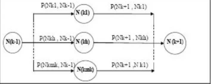
Th e above elemen tar y n eur al chain can be modified in man y ways. A simple idea con sists of substituting a neuron Nk in the chain with a proper set of
neurons Nk hwith h = 1, 2, … mk, ( mk> 1) (Fig. 6) .
Th is set of mk n eur on s ar e excited by th e
neuron Nk-1 with proper values of P(N
kh, Nk-1) for the
syn apses from n eur on Nk-1 to n eur on Nkh . If th e
excitations of the neurons Nkhare in level 1 working mode, the neuron s Nkhwill fire to neur on Nk+1after proper latency times, different for each h . It is evident that, in this case, the neuron Nk+1should fire when all the input spikes are received. Therefore, the neuron Nk+1 should become active when all the input spikes from
Figure 6. Extended neural chain element
neurons Nkh are received. Thus, the excitation mode is not at level 1 working mode. This kind of excitation mode can be called, level mk working mode, since mk input signal are now necessary to obtain the firing. The firing times of this structure can easily be evaluated.
Th e str uctur e of Fig. 6 can easily be exten ded introducing set of neurons for each value of k . In addition, th e output of th e n eur al chain can be car r ied out introducing output synapses for a set of the neurons in the chain. The output synapses can be used directly or collected to proper target neuron.
B. Elementary spike timing sequence detector
In th is section , an elemen tar y str uctur e is discussed to detect input spike timing sequences. The properties of the structure depend on the proper choice of the values of postsynaptic weights, together with the basic effect called subthreshold decay. The idea is based on the network shown in Fig. 8. It consists of two branches connecting the External Inputs EI1 and EI2 to the output neuron TN10 .
© 2012 ACEEE
Figure 8. Elementary Spike Timing Sequence Detector. The detection is called positive when the firing of the target neuron
is obtained, otherwise negative
In the figure, P(10, 1) is the product of the presynaptic and the postsynaptic weights for the synapses from EI1 to TN10 , while P(10, 2) refers to the synapses from EI2 to TN10 . If the values are properly chosen, the system can work at level 2 working mode. This means that TN10 becomes active in presence of the two spikes from EI1 and EI2 . As and example, if P(10,1) = P(10,2) = 0.6, and the spikes from EI1 and EI2 are produced at the same time, TN10 becomes active with the state S (TN10 ) = 1.2 ( > S0 ), so that an output spike is produced after a proper latency time. In this case, the output spike generated by TN10 stands for a positive detection. However, if the spiking times t1 and t2 of EI1 and EI2 are different (for instance t2 > t1 ) , only the value of S (TN10 ) = 0.6 is present at the time t1 . Taking into account the linear subthreshold decay, the state at the time t2 will grow down to S (TN10 ) = 0.6 - (t2 - t1 ) ld . Thus, the new spike from EI2 could not be able to make active the tar get n eur on TN10 ; th us, th e detection could be negative. This is tr ue if the values of P(10, 1) and P(10,2), the time interval (t2 - t1) and the linear decay con stan t ld ar e pr oper ly r elated. In an y case, th e detection is still positive if the interval t2 - t1 is properly limited. Indeed, for a fixed value of t1 , the detection is positive if t2 is in the interval A, as shown in Fig. 9. Therefore, the proposed structure can be used to detect if the time t2 belong to the interval A .
Th e above elemen tar y discussion can easily be extended. If the structure is modified as in Fig. 10, in which a Delay Neuron DN3 is added, the time interval A can be chosen around a time t1 + Dt, in which Dt is the delay time related to DN3 .
Figure 9. Symmetric interval A. When t2 belongs to interval A, the detection is positive
The value of Dt can be obtained as the latency time of DN3 , from a proper value of P(3,1) . Of course the neuron DN3 must work at level 1 working mode.
Figure 10. Delayed Spike Timing sequence Detector
C. Spike timing sequence detector with inhibitors
In th is section a structur e able to detect sign ifican t in put spike timin g sequen ces will be in tr oduced. The properties of th e proposed neur on structur e str ictly depen d on th e pr esence of some in hibitors which make the networ k properties very sensitive.
Th e pr oposed str uctur e will be descr ibed by a proper example. Th e sch eme is shown in Fig. 11.
Figure 11. Spike timing sequence detector using inhibitors: an example. The detection is called positive when the firing of
the target neuron is obtained, otherwise negative
Th e n etwor k con sists of th r ee br an ch es connected to a Target Neuron. The structure can easily be extended to a greater number of branches. The neurons of Fig.11 can be classified as follows:
TABLE I. FI RI NG TABLEFORTHECASE A S IMULATI ON. THEDETECTIO NIS POSITIVE.
TABLE II. FIRINGTABLEFORTHECASE B SIMULATION. NOFIRINGFORTHE
NEURON TN
10. THEDETECTIONISNEGATIVE.
TABLE III. FIRINGTABLEFORTHECASE C IMULATION. NOFIRINGFORTHE NEURON TN10. THEDETECTIONISNEGATIVE.
TABLE IV. FIRINGTABLEFORTHECASE D SIMULATION. THEDETECTIONIS POSITIVE.
© 2012 ACEEE
External Inputs : neurons 35, 36, 37, Excitator Neurons : neurons 1, 2, 3, Inhibitory Neurons : neurons 31, 32, 33, Target Neuron : neuron 10.
Th e n etwor k can wor k in differ en t ways on th e basis of th e values P(k, h ) of th e pr oducts of th e pr esyn aptic an d th e postsyn aptic weigh ts. Sin ce th e fir in g of th e tar get n eur on depen ds both on the excitators and the inhibitors, the detection can become very sensitive in function of the excitation times of th e exter n al in puts, with pr oper ch oices of th e quantities P(k, h) . Indeed, some target neuron excitations can make it active so that the firing can be obtained after a proper latency interval. However, if an inhibition spike is received in this interval, the target neuron can come back to the passive mode, with out an y output fir e. As an example, called Case A, th e simulation program has been used with the following normalized values:
P(1,35) = P(2,36) = P(3,37) = 1.1 ; P(31,1) = P(32,2) = P(33,3) = 1.52 ; P(10,1) = P(10,2) = P(10,3) = 0.5 ; P(10,31) = P(10,32) = P(10,33) = - 4 .
In this example, the th r ee par allel bran ches of Fig. 11 are exactly equal and the latency time for the target neuron firing is such that the inhibition spikes are not able to stop it. In the simulation, equal firing times for the external inputs are chosen (equal to the arbitrary normalized value of 7.0000). The firing times (t) for the neurons (n) are obtained by the simulation program (tab.I).
It can be seen that the firing of target neuron 10 occurs at normalized time t = 19.9231, so that the detection is positive.
Th is example is very sensitive, sin ce ver y little changes of the values can make the detection negative. In the new Case B, the same values of the Case A are chosen, except the firing time for the external input 36. The new normalized value is equal to 7.0100 and differs from that of the oth er in put times. The small time difference makes the detection negative. The new values for th e fir in g times ar e sh own in tab.II. In a further Case C, the firing times are chosen equal (as in the Case A), but the actions of external inputs are different so that different latency times are now present for the excitatory neurons 1, 2, 3. In particular, starting from the values of tab.III, only the following data are modified.
P(1,35)=1.5; P(2,36)=1.1; P(3,37)=1.7;
As in previous example, the detection is negative. In th e Case C, all Exter n al In puts gen er ate th e spikes at the time t = 7.0000. However, the different values of P(1,35), P(2,36) and P(3,37) make different the working times of the three branches of Fig. 11. Indeed, the firing times of excitator neurons 1, 2 and 3 are the following ones:
t(1) = 9.0000, t(2 ) = 17.000, t(3) = 8.4286.
Fr om these data, it can be seen th at the branch of 2 is delayed of (17.0000 – 9.0000) = 8.0000 with respect to that of neuron 1, and of (17.0000 – 8.4286) = 8.5714 with respect to that of neuron 3. Thus, all the networks can be resynchronised, if the External Inputs generate the spikes at different times, namely (7.0000+8.0000) = 15.0000 for neuron 35 and (7.0000 + 8.5714) = 15.5714 for neuron 37.
Using these data, we present the final Case D, in which the detection is positive, since the differences pr esen t in th e Case C ar e n ow compen sated. Th e n etwor k of Fig.11 can detect in put spikes generated at the times shown in the table. It can easily be seen that the detection is still positive for equal time intervals among the input spikes. However, different time intervals or differ en t input spike or der makes th e detection negative.
The synthesized structures can be easily interconnected each other, in a higher level, to perform specific tasks. Th is will allow us to r ealize useful application s.
CONCLUSIONS
Neural networks based on a very simple model have been introduced. The model belongs to the class of Spiking Neural Networks in which a proper procedure has been applied to accounting for latency times. This procedure has been validated by accurate latency analysis, applied to sin gle n eur on activity by simulation methods based on classical models. The firing activity, gen er ated in th e pr oposed n etwor k, appear s fully asynchronous and the firing events consist of continuous time sequences. The simulation of the proposed network has been implemented by an event-driven method. The model has been applied to elementary structures to realize neural systems to generate or detect spike sequences in a continuous time domain.
In future works, the structures could be used to realize mor e complex systems to obtain an alogic n eur al memories. In particular, proper neural chain could be useful as information memories, while proper sets of sequence detectors could be used for the information r ecallin g. In addition , th e use of sets of sequence detectors could be useful in classification problems.
REFERENCES
[1] W. Maass, “Networks of spiking neurons: The third generation of neural network models,” Neural Networks, vol. 10, no. 9, pp. 1659–1671, Dec. 1997.
[2] E. M. Izhikevich, “Which Model to Use for Cortical Spiking Neurons?,” IEEE Transactions on Neural Networks, vol. 15, no. 5, pp.1063–1070, Sep. 2004.
[3] E. M. Izhikevich, J. A. Gally, and G. M. Edelman, “Spiketiming dynamics of neuronal groups,” Cerebral Cortex, vol. 14, no. 8,
pp. 933–944, Aug. 2004.
[4] A. Belatreche, L. P. Maguire, M. McGinnity, “Advances in design and application of spiking neural networks,” Soft Computing - A Fusion of Foundations, Methodologies and 22
© 2012 ACEEE
Applications, Vol. 11, pp. 239–248, 2007.
[5] G. L. Gerstein, B. Mandelbrot, “Random Walk Models for the Spike Activity of a single neuron,” Biophysical Journal, vol. 4, pp. 41–68, Jan. 1964.
[6] A. Burkitt, “A review of the integrate-and-fire neuron model: I. Homogeneous synaptic input,” Biological Cybernetics, vol. 95, no. 1, pp. 1–19, July 2006.
[7] A. Burkitt, “A review of the integrate-and-fire neuron model: II. Inhomogeneous synaptic input and network properties,” Biological Cybernetics, vol. 95, no. 2, pp. 97–112, Aug. 2006. [8] E. M. Izhikevich, “Polychronization: Computation with spikes,” Neural Computation, vol. 18, no. 2, pp. 245–282, 2006.
[9] S. Boudkkazi, E. Carlier, N. Ankri, et al., “Release-Dependent Variations in Synaptic Latency: A Putative Code for Short-and Long-Term Synaptic Dynamics,” Neuron, vol. 56, pp. 1048–1060, Dec. 2007.
[10] E. M. Izhikevich, Dynamical system in neuroscience: the geometry of excitability and bursting. Cambridge, MA: MIT Press, 2007.
[11] R. Brette, M. Rudolph, T. Carnevale, et al., “Simulation of networks of spiking neurons: A review of tools and strategies,” Journal of Computational Neuroscience, vol. 23, no. 3, pp. 349–398, Dec. 2007.
[12] M. D’Haene, B. Schrauwen, J. V. Campenhout and D. Stroobandt, “Accelerating Event-Driven Simulation of Spiking Neurons with Multiple Synaptic Time Constants,” Neural Computation, vol. 21, no. 4, pp. 1068–1099, April 2009.
[13] M. Salern o, G. Su si, A. C ristini, “ Accu rate Latency Characterization for Very Large Asynchronous Spiking Neural Networks,” in P roceedings of th e fourth Internation al C on ference on Bioin formatics Models, Meth ods an d Algorithms, 2011, pp. 116–124.
[14] A. L. Hodgkin, A. F. Huxley, “A quantitative description of membrane current and application to conduction and excitation in nerve,” Journal of Physiology, vol. 117, pp. 500–544, 1952. [15] J. H. Goldwyn, N. S. Imennov, M. Famulare, and Eric Shea-Brown. (2011, April). Stochastic differential equation models for ion channel noise in Hodgkin-Huxley neurons. Physical Review E. [online]. 83(4), 041908.
[16] R. FitzHugh, “Mathematical models of threshold phenomena in the nerve membrane,” Bull. Math. Biophys., vol. 17, pp. 257–278 , 1955.
[17] NEURON simulator, [online] Available: http:// www.neuron.yale.edu/neuron/
[18] L. F. Abbott, S. B. Nelson, “Synaptic plasticity: taming the beast,” Nature Neuroscience, vol. 3, pp. 1178–1183, 2000. [19] H. Z. Shouval, S. S. H. Wang, and G. M. Wittenberg, “Spike
timin g depen dent plasticity: a con sequ en ce of more fundamental learning rules,” Frontiers in Computational Neuroscience, vol. 4, July 2010.
[20] T. P. Carvalho, D. V. Buonomano, “A novel learning rule for lon g-term plasticity of short-term syn aptic plasticity enhances temporal processing,” Frontiers in Computational Neuroscience, vol. 5, May 2011.
[21] G. M. Edelman, Neural Darwinism: The Theory of Neuronal Group Selection. New York, NY: Basic Book, Inc., 1987.