A Python data analysis library for genomics and its application to biology

(1)

POLITECNICO DI MILANO

School of Industrial and Information Engineering Master of Science in Computer Science and Engineering Department of Electronics, Information and Bioengineering

A PYTHON DATA ANALYSIS LIBRARY

FOR GENOMICS AND ITS

APPLICATION TO BIOLOGY

Laboratory of Bioinformatics and Web Engineering

Supervisor: Prof. Stefano Ceri Co-supervisor: Dott. Pietro Pinoli

Second supervisor (Politecnico di Torino): Elena Baralis

Master Thesis of: Luca Nanni, Matr 850113

(2)

(3)

(4)

(5)

Abstract

Genomics is the study of all the elements that compose the genetic material within an organism. The new DNA sequencing technologies (NGS) have opened new lines of research, which include the study of diseases like cancer or genetic conditions. The huge amount of data produced by these new methods makes the genomic data management one of the current biggest big data problems.

In this context, GMQL, a declarative language built on top of big data technologies, was developed by the Bioinformatics group at Politecnico di Milano.

The first aim of this thesis is to enlarge the scope of this language by designing and implementing a Python package capable of interfacing with the big data engine, to extract the results and convert them in a useful data structure and to give the user the possibility to work with GMQL in a full interactive environment. The package will be able to perform computations both on the local machine and using a remote GMQL server and will interface with the main data science and machine learning python packages.

The second focus of this work is on applying the developed package to concrete biological problems. In particular we will concentrate on the study of Topologically Associating Domains (TADs), which are genomic regions within which the physical interactions occur much more frequently than out of them. We will use the package to analyze these data, extract new knowl-edge about them and derive their physical properties.

(6)

(7)

Sommario

La genomica è lo studio di tutti gli elementi che compongono il materiale genetico di un organismo. Le nuove tecnologie di sequenziamento del DNA (NGS) hanno aperto, negli ultimi anni, nuove frontiere di ricerca fra cui lo studio dei tumori e delle malattie ereditarie su larga scala. La grande quantità di dati prodotti da questi nuovi metodi rendono la gestione di dati genomici uno dei problemi più grandi nel campo dei big data.

In questo contesto, presso il laboratorio di bioinformatica e web engi-neering del Politecnico di Milano è stato sviluppato il sistema GMQL, che consiste in un linguaggio dichiarativo il quale, utilizzando tecnologie di pro-cessamento big data, permette l’esecuzione di query genomiche su grandi moli di dati.

Lo scopo primario di questa tesi è di estendere questo linguaggio at-traverso il design e l’implementazione di una libreria python che possa in-terfacciarsi con il sistema di processamento dati, estrarre i dati di interesse, convertirli in una struttura dati efficiente e rappresentativa e infine fornire un ambiente di sviluppo interattivo. La libreria sarà anche in grado di eseguire localmente o tramite l’utilizzo di un cluster remoto, nonché potrà interfac-ciarsi con le principali librerie python di data science e machine learning.

In secondo luogo, la libreria verrà testata direttamente nella risoluzione di complessi problemi biologici. In particolare verrà posta l’attenzione sullo studio dei domini topologici, i quali sono particolari regioni genomiche carat-terizzate da un aumentata densità di interazioni fisiche. Durante lo studio si utilizzerà la libreria per analizzare i dati ed estrarne nuova conoscenza al fine di derivare le proprietà fisiche di queste particolari regioni.

(8)

(9)

Ringraziamenti

Naturalmente non posso che iniziare i miei ringraziamenti ringraziando il mio relatore Stefano Ceri e il mio corelatore Pietro Pinoli, che mi hanno seguito, incoraggiato e sempre sostenuto in questo percorso. Un forte ringraziamento anche a tutto il gruppo di bioinformatica presso il quale ho lavorato in questi ultimi mesi e in particolare Arif e Abdo, che mi hanno sempre aiutato in caso di bisogno. Ringrazio inoltre Michele, Andrea, Ilaria B., Ilaria R., Eirini.

Un ringraziamento particolare ai ragazzi del gruppo dell’Alta Scuola Po-litecnica, che mi hanno seguito e sopportato in questi due anni di lavoro: Gianluca, Paolo, Diletta, Flavio e Antonio.

Un particolare ringraziamento naturalmente va a Francesco, Riccardo, Filippo, Lorenzo, Andrea, Mirco, Giacomo, Francesca, Lisa, Ezia, senza i quali probabilmente tutto quello che ho fatto finora non avrebbe significato. Un grazie a i miei coinquilini, che in questi due anni mi hanno sopportato e hanno riso con me: Ale, Lorenzo ed Elia.

E come nei più classici ringraziamenti, ma soprattutto perché è la verità, il più grande ringraziamento va a tutta la mia famiglia, che mi ha sostenuto in tutto e per tutto da sempre.

E (perchè no?) un grazie anche a me stesso, che ha sempre guardato avanti e cercato di migliorarsi ad ogni passo lungo questa difficile, ma bellis-sima esperienza.

(10)

(11)

List of Figures

1.1 The DNA structure. Taken from [14] . . . 2

1.2 Time-line of the Human Genome Project. Taken from [4]. . . 3

1.3 Differences between Primary, Secondary and Tertiary analy-sis. Taken from [20]. . . 4

1.4 The role of GMQL in the genomic data analysis pipeline. Taken from [16] . . . 4

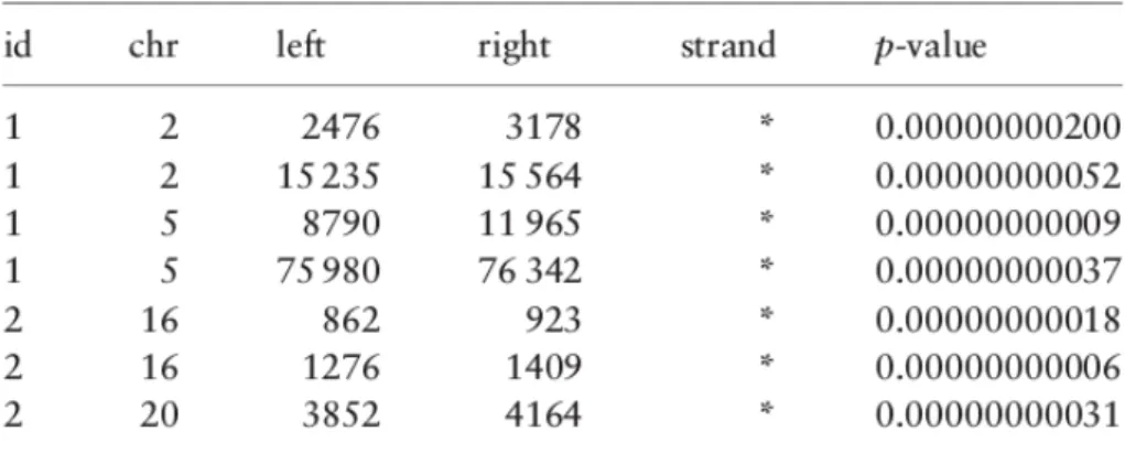
2.1 A part of region data from a dataset having two ChIP-Seq samples . . . 11

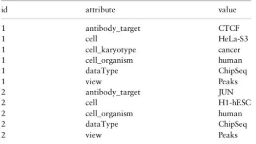
2.2 A part of metadata from a dataset having two ChIP-Seq sam-ples. These metadata correspond to the samples shown in figure 2.1 . . . 12

2.3 Accumulation index and COVER results with three different minAcc andmaxAcc values. . . 18

2.4 Example of map using one sample as reference and three sam-ples as experiment, using the Count aggregate function. . . . 20

2.5 Different semantics of genometric clauses due to the ordering of distal conditions; excluded regions are gray. . . 23

2.6 First version of GMQL. The architecture. . . 27

2.7 Current architecture of GMQL. Taken from [19] . . . 28

2.8 Command line interface for sending GMQL queries.. . . 29

2.9 Example of web interface usage for GMQL . . . 30

2.10 Complete abstract DAG for the query. . . 34

3.1 Process of compilation of a Scala program . . . 36

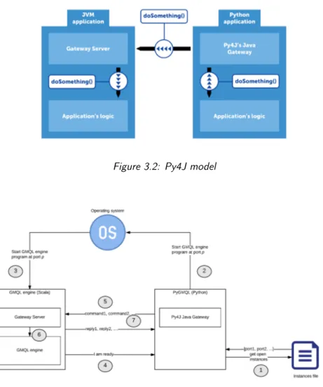
3.2 Py4J model . . . 41

3.3 Process of creation of the Scala back-end and interaction with PyGMQL. . . 41

3.4 Steps in the Spark Submit mode of execution . . . 42

3.5 High level diagram of the first architecture proposal. . . 45

(16)

3.7 High level diagram of the third architecture proposal . . . 48

4.1 High level view of the whole GMQL system. . . 50 4.2 Architecture of the PyGMQL package . . . 51 4.3 Main interactions between the Python library and its Scala

back-end . . . 52 4.4 An example of programming work-flow using PyGMQL. . . . 53 4.5 The process of materialization depending on the execution

mode of PyGMQL. In the image we can see both the execution at the API level and at the server level. Each square represents a step and the arrows represent information exchange. . . 55 4.6 Example of DAG renaming where the server has to rename

the dataset names, in all the loading nodes, to Hadoop file system paths . . . 57 4.7 PyPi work-flow from the point of view of both the package

maintainer and final user. . . 58

5.1 Interaction between a GMQLDataset and the Scala back-end for storing the variable information . . . 60 5.2 Visual representation of the region data and the metadata

structures in a GDataframe. Notice how the sample ids must be the same and coherent in both the tables. . . 69 6.1 Schematic representation of the Hi-C method . . . 77 6.2 Schematic representation of two TADs and the boundary

be-tween them. Taken from [11] . . . 78 6.3 Descriptive data about the two TADs dataset used in the study 79 6.4 Distribution of sizes in the two TADs dataset used in the study 80 6.5 Schematic illustration of the gene expression process . . . 80 6.6 Distribution of samples in the different tissues present in the

GTEx database . . . 82 6.7 Comparison of gene correlation in the same and cross sets in

the brain tissue, using TADs from [11] . . . 85 6.8 Comparison of gene correlation in the same and cross sets in

the ensemble of brain, breast and liver tissues, using TADs from [11]. . . 85 6.9 Comparison of gene correlation in the same and cross sets in

the muscle tissue, using TADs from [11] . . . 85 6.10 Comparison of gene correlation in the same and cross sets in

(17)

6.11 Comparison of gene correlation in the same and cross sets in the ensemble of brain, breast and liver tissues, using TADs from [26]. . . 87 6.12 Comparison of gene correlation in the same and cross sets in

the muscle tissue, using TADs from [26] . . . 87 6.13 Some example in four tissue/tumor comparison. Red dashed

line: tumor same. Blu dashed line: tumor cross. Red contin-uous line: normal same. Blu contincontin-uous line: normal cross . . 88 6.14 Comparison of gene correlation in the same and cross sets

in the ensemble of brain, breast and liver tissues, using the mouse TADs . . . 92 6.15 Example of a ChIA-PET dataset as two GMQL dataset with

a common id column . . . 93 6.16 Visualization of the dendrogram of the hierarchical clustering

with a cutting point at distance 350 . . . 95 6.17 Aggregate statistics for the found clusters using the

(18)

(19)

List of Tables

3.1 Table of the main soft requirements and hard requirements of the Python API for GMQL . . . 43 3.2 Table of the main users of the library. . . 44 5.1 Mapping between the GMQL aggregate operator and their

equivalent in PyGMQL. . . 63 5.2 Mapping between the genometric predicates of GMQL and

the ones of PyGMQL. . . 64 6.1 Cell lines for each TAD dataset considered in the study . . . 79 6.2 For each tumor type the difference of correlation between the

normal and tumor tissue. . . 89 6.3 Cluster statistics for the gene expression clustering . . . 96

(20)

Chapter 1

Introduction

”Frankly, my dear, I don’t give a damn.”

Gone with the wind

1.1 Genomics and the Human Genome Project

With the term Genomics we mean the study of all the elements that compose the genetic material within an organism [21].

The most important chemical structure studied in genomics is the De-oxyribonucleic acid (DNA). This chemical compound contains all the infor-mation needed to guide, develop and support the life and development of all the living organisms. DNA molecules are composed of two twisting paired strands. Each strand is made of four units called nucleotide bases (Adenine, Timine, Guanine, Cytosine): these bases pair each other on the two strands following specified rules (A - T, C - G). The information is encoded in the DNA by the order in which these bases are placed in the molecule.

A gene is a portion of DNA that is taught to carry the information used to build a (set of) protein(s). Proteins are large molecules having a lot of different functions and one of the most important molecular structure for living organisms.

The genes are packed into larger structures called chromosomes. These big sections of DNA are paired together: for example, in the human organism we have 23 pairs of chromosomes.

In figure 1.1we can see the full structure of the DNA.

The study of genes and their role on the expression of human traits is one of the main problems of modern medical research. Genes and their mutations

(21)

Figure 1.1: The DNA structure. Taken from [14]

have been proven to be at the base of several diseases. In particular in these years the subfield of cancer genomics is getting a lot of attentions. Computations biologists, geneticists and cancer researchers are looking at the genome level in order to understand the low level interactions leading to the development of tumors.

These new lines of research are now possible thanks to the new tech-nologies for DNA sequencing. Sequencing the DNA means to determine the exact order of the bases in a strand of it [21]. From the 1990 to 2003 an international project called Human Genome Project was carried out with the aim to develop sequencing techniques for the full mapping of the human genome (see figure 1.2for a time-line of the project).

The project was a success and in the first decade of the new millennium a new sequencing paradigm was developed, called Next Generation Sequenc-ing. NGS enabled high-throughput, high-precision and low-cost sequencing making the DNA mapping a standardized process.

(22)

Figure 1.2: Time-line of the Human Genome Project. Taken from [4]

1.2 Big data in biology and genomics

NGS technologies and the success of the human genome project opened a new era in genomics. Never before such a great amount of data was publicly available for conducting biological research.

Of course the high volume of data produces a wide range of technical problems:

• Storage: data must be stored in public accessible databases

• Heterogeneity: data can have a potentially infinite number of formats

• Computational power : analyzing the data and applying algorithms to them must take into account their cardinality

These problems and the requirements that they produce configure the analysis of genomic data as one of the biggest and most important current big data problem.

The analysis of genomic data can be divided in three main categories, as explained in figure1.3. Primary analysis deals with hardware generated data like sequence reads. It is the first mandatory step for extracting information from biological samples. Secondary analysis takes the reads of the previous step and filters, aligns and assembles them in order to find relevant features. Tertiary analysis works at the highest level of the pipeline and it is dedicated to the integration of heterogeneous data sources, multi-sample processing or enrichment of the data with external features.

(23)

Figure 1.3: Differences between Primary, Secondary and Tertiary analysis. Taken from [20]

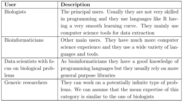
Figure 1.4: The role of GMQL in the genomic data analysis pipeline. Taken from [16]

1.3 Motivations and requirements

In this thesis we will address the problem of organizing, explore and analyze tertiary genomic data. In particular we will implement and use a python package for manipulating such data. We will design this library on the basis of the already existent GMQL system, which is a big genomic data engine developed at the Department of Electronics, Information and Bioengineering of the Politecnico of Milano (see figure 1.4). This python package will be validated through testing and also by applying it to a specific biological research problem. This will demonstrate the quality of the product, its usefulness and its applicability to a wide range of problems.

(24)

Biologists and researchers in genomics usually organize their work-flow in pipelines. A pipeline is a chain of operations applied to a set of data. Usually researchers work with files locally in their computer or in a local server and use the most common programming languages or frameworks for data analysis (Python, Perl, Matlab, ecc...). The problem of this approach is the low scalability and the implicit difficulty in the writing of a good, reliable and repeatable algorithm.

Therefore in this work we focused on the development of an integrated python environment having the following main characteristics

• Ease of use: biologists and researchers must be able to use this soft-ware even without solid computer science background. Therefore the complexity of the algorithms must be encapsulated into atomic and semantically rich operations.

• Efficient processing: The package must be able to interface to big data processing engines. This is a very crucial point as data used in tertiary analysis are often too big to be handled locally by the user machine. In particular, as we have said, we will interface with the GMQL sys-tem which will provide the computational power for doing genomic operations on big data.

• Data Browsing and exploration: this requirements comes directly from the previous one. Since we are dealing with high volumes of data, we must provide a way to explore them easily in order to understand the best pipeline.

• Personalization: the user must be able to define arbitrary complex pipelines using the atomic operations provided by the package.

We will apply this package to an open biological problem, which is the study of Topologically Associated Domains (TADs). TADs are large locations of the genomes that are thought to carry functional information. We will try to extract information about TADs by clustering them based on the expression profiles of the genes inside them.

1.4 The Python library in a nutshell

From the above requirements and through a design process that evaluated different solutions (which can be found in section3.5) we developed a python package called PyGMQL.

(25)

The package place itself above the GMQL engine and exploits it using its Scala API or through a remote REST interface. The library therefore enables the user to operate in two different modes: in local mode the execution is performed in the user machine like any other python package; in remote mode the query is sent to the remote server and the results are downloaded, when they are ready, to the local machine at the end of execution. This creates some coherency problems that we will describe later with their solution.

Each GMQL operator has been mapped to an equivalent python function to be applied to a GMQLDataset, which represents the python abstraction of a GMQL variable.

An appropriate data structure for holding the query results has been designed. In particular this structure, the GDataframe, is very useful for performing python specific tasks or applying machine learning algorithms. A Machine Learning module is being currently developed by Anil Tuncel for his master project.

In chapter 4 we will deepen into the implementation and specifications of the python library.

1.5 Biological application

The effectiveness of the library was evaluated through its direct application to some biological problems. As first thing we applied it to some known bio-logical problems that were already addressed by the classical GMQL system. After this, a very complex and open biological problem was addressed: the understanding of the functional role of Topologically associating domains, which are genomic regions within which the physical interactions occur much more frequently than out of them.

We approached this problem by studying the relationship between these regions and the gene inside of them. We compared the correlation of genes in the same TAD with respect to genes across different TADs. We did this operation also considering tumor and normal expressnion profiles for the same gene.

We discovered a strong relationship between gene expression and TADs: genes on the same TAD show an higher correlation than across them. Addi-tionally, the correlation increases when we substitute the normal expression profile with the tumor one.

We also analyzed the intersection between human and mouse TADs in order to prove their conservation across different species reaching a coverage of 60%.

(26)

Finally we performed cluster analysis of TADs by using expression profiles and ChIA-PET links (which are basically protein binding sites connections across the genome). We show how TADs can be clustered together and the characteristics of the clusters.

In chapter 6can be found a deep explanation of these problems and the biological pipelines that were setup for solving them.

1.6 Outline of the work

This document is structured as follows:

• Chapter 2: we will give a deep background about the GMQL system. This part is fundamental in order to understand the design choices and the different architectures that were proposed and evaluated during the process.

• Chapter 3: we will deepen into the problems that making interact a python package with a Scala one. The proposed solution for exchang-ing data between the two languages is presented. Since GMQL is a declarative language that works in a batch execution, we will present also the problems in shifting this paradigm to an interactive and pro-grammatic one.

• Chapter 4: here we will present the full architecture of the python module and the Scala back-end

• Chapter 5: we will deepen into the mapping between GMQL opera-tors and python functions, also describing the defined data structures holding the results of a query

• Chapter 6: the final part of the work will explain the TADs problem and how the developed library was used to analyze it and trying to address important biological questions.

• We will conclude with an overview of the possible future enhancements and new research lines that can be opened.

(27)

(28)

Chapter 2

Background

”I’m gonna make him an offer he can’t refuse.”

The Godfather

In this chapter we will deepen into the features, the architecture and the design of the Genometric Query language (GMQL). This will serve as a starting point for the next sections in which we will explain the process and the solution that has been designed on top of this technology.

In particular we will explain the following concepts:

1. The Genomic Data Model: a formal framework for representing ge-nomic data

2. The Genometric Query Language: a declarative language that gives the user the ability to perform queries on the data defined in the Genomic Data Model

3. The system architecture: the kind of services that are offered and their limitations

4. The query execution strategy: how a submitted query is executed

2.1 Genomic Data Model

We have seen that in biology and genomics there is a huge variety of data formats. The Genomic Data Model (GDM) tries to abstract the file format and represents genomic data as the combination of two kinds of information: • Region data: the physical coordinates of the considered genome zone with the addition of specific fields having different value for each region. A set of regions is called a sample.

(29)

• Metadata: descriptive attributes of a sample (set of regions). They de-scribe the biological, clinical and experimental properties of the sample. It must be noticed that while for the region representation there exist several data formats, there is no agreed standard for modeling metadata. In GDM metadata are modeled as attribute-value pairs. There is total freedom in the definition of both the attributes and the values1.

Region data, in order to be comparable between different datasets, should follow some rules defining their structure: these rules are encoded in a schema. Each GDM dataset has a schema and it must include at least the following information: the chromosome, the start and end positions of the region (encoded as an integer number). Optional parameter is the strand, which represents the direction of DNA reading.

2.1.1 Formal model

In [20] a formal definition of the GDM is provided. Here we will report it and deepen into the various design choices.

The atomic unity of a GDM dataset is the genomic region. A region is defined by a set of coordinates

c =< chr, lef t, right, strand > and a set of features

f =< f eature1, f eature2, ..., f eatureN >

The concatenation of these two arrays of values creates the region r =< c, f >

The order of the coordinates and the features is fixed in all the regions of a dataset and it is dictated by the schema. In addition, these fields are all typed (for the coordinates we have respectively string,integer,integer,string).

On the other side, metadata are arbitrary attribute-value pairs < a, v >. It must be noticed that the same attribute can appear multiple times in the same sample. This is allowed due to the need of specify, in some dataset, multiple conditions for the same metadata (for example adiseasemetadata could have multiple values for the same patient).

A set of regions is called sample and it is structured like follows: s =< id, {r1, r2, ...}, {m1, m2, ...} >

(30)

Figure 2.1: A part of region data from a dataset having two ChIP-Seq samples

Each sample is therefore identified by an id, which is unique in all the dataset. A sample has multiple regions ri and multiple attribute-value pairs of

meta-data mi.

A GDM dataset is simply a set of samples having the same region schema and a sample id which is unique. This identifier provides a many-to-many connection between regions and metadata of a sample. In figure2.1and2.2 we can see the relations between the metadata and the region data in the GDM.

2.2 Genometric query language

Having defined the data model we now have to explain how to query this kind of data. The language that enables us to do so is called GMQL (GenoMet-ric Query Language). It is a declarative language inspired by the classical languages for database management [20].

GMQL extends the conventional algebraic operations (selection, projec-tion, join, etc...) with domain specific operations targeting bioinformatics applications. The main objectives of the language are:

• Provide a simple and powerful interface for biologists and bioinformati-cians to huge dataset enabling them to explore and combine heteroge-neous sources of informations.

• Being highly efficient and scalable

• Being as general as possible in order to tackle a great variety of prob-lems and biological domains

(31)

Figure 2.2: A part of metadata from a dataset having two ChIP-Seq samples. These metadata correspond to the samples shown in figure2.1

We can express a GMQL query as a sequence of statements crafted as follows [16]:

<var> = operation(<parameters>) <vars>

Each<var>is a GDM dataset and operations can be unary or binary and returns one result variable.

The resulting dataset will have inherited or new generated id s depending on the operation.

The declarative nature of the language implies that the user needs to specify the structure of the results and he does not care about the imple-mentation of the operations.

2.3 GMQL operations

We can divide the set of operations in GMQL in two sets:

• Relational operations: these are classical operators that can be found in all the classical data management systems (SELECT,PROJECT, EXTEND, MERGE,GROUP,SORT,UNION and DIFFERENCE)

• Genomic-specific operations: designed to address the specific needs of biological applications (COVER,MAP andJOIN).

(32)

2.3.1 Relational operators

Select

<S2> = SELECT([SJ_clause ;][<pm>][; <pr>]) <S1>

It keeps in the result all the samples which existentially satisfy the metadata predicate<pm>and then selects those regions of selected samples which satisfy the region predicate<pr>. The result will have ids belonging to S1.

We can use semi-join clauses to select the samples using informations from an other dataset. They have the syntax: <A> IN <extV>. The predicate is true for a given sample si of S1 with attribute ai iff there exists a sample

in the variable denoted asextV with an attribute aj and the two attributes

ai and aj share at least one value. Formally, if ME denotes the metadata of

samples ofextV, then:

p(ai, aj) ⇐⇒ ∃ (ai, vi) ∈ Mi, (aj, vj) ∈ ME : vi = vj

Semi-joins are used to connect variables, e.g. in the example below: OUT = SELECT(Antibody IN EXP2) EXP1

which requests that the samples of EXP1 are selected only if they have the same Antibodyvalue as at least one sample of EXP2.

Project

<S2> = PROJECT([ <Am1> [AS <f1>], .., <Amn> [AS <fn>]] [; <Ar1> [AS <f1>], .., <Arn> [AS <fn>]]) <S1>

It keeps in the result only the metadata (Am) and region (Ar) attributes ex-pressed as parameters. New attributes can be constructed as scalar expres-sions fi. If the name of existing schema attributes are used, the operation updates region attributes to new values. Identifiers of the operand S1 are assigned to the result S2.

Extend

<S2> = EXTEND ( <Am1> AS <g1>, .., <Amn> AS <gn> ) <S1>

It creates new metadata attributes Am as result of aggregate functions g, which is applied to region attributes; aggregate functions are applied sample by sample. The supported aggregate functions includeCOUNT(with no argu-ment), BAG(applicable to attributes of any type) and SUM, MIN, MAX, AVG, MEDIAN, STD. In the example below:

(33)

OUT = EXTEND (RegionCount AS COUNT, MinP AS MIN(Pvalue)) EXP

for each sample ofEXP, two new metadata attributes are computed,RegionCount as the number ofsample regions, and MinP as the minimum Pvalue of the sample regions. Group <S2> = GROUP([<Am1>..<Amn>; <Gm1> AS <g1>, .., <Gmn> AS <gn>] [; <Ar1>..<Arn>; <Gr1> AS <g1>, .., <Grn> AS <gn>]) <S1>;

It is used for grouping both regions and metadata according to distinct val-ues of the grouping attributes. For what concerns metadata, each distinct value of the grouping attributes is associated with an output sample, with a new identifer explicitly created for that sample; samples having missing values for any of the grouping attributes are discarded. The metadata of output samples, each corresponding a to given group, are constructed as the union of metadata of all the samples contributing to that group; conse-quently, metadata include the attributes storing the grouping values, that are common to each sample in the group. New grouping attributes Gm are added to output samples, storing the results of aggregate function evalua-tions over each group. Examples of typical metadata grouping attributes are the Classification of patients (e.g., as cases or controls) or their Disease values.

When the grouping attribute is multi-valued, samples are partitioned by each subset of their distinct values (e.g., samples with a Disease at-tribute set both to ’Cancer’ and ’Diabetes’ are within a group which is distinct from the groups of the samples with only one value, either’Cancer’ or ’Diabetes’). Formally, two samples si and sj belong to the same group,

denoted as s_iγAsj, if and only if they have exactly the same set of values for

every grouping attribute A, i.e.

siγAsj ⇐⇒ {v|∃(A, v) ∈ Mi} = {v|∃(A, v) ∈ Mj}

Given this definition, grouping has important properties: • reflexive: siγAsi

• commutative: siγAsj ⇐⇒ sjγAsi

(34)

When grouping applies to regions, iby default it includes the grouping at-tributeschr, left, right, strand; this choice corresponds to the biological application of removing duplicate regions, i.e. regions with the same coordi-nates, possibly resulting from other operations, and ensures that the result is a legal GDM instance. Other attributes may be added to grouping attributes (e.g., RegionType); aggregate functions can then be applied to each group. The resulting schema includes the attributes used for grouping and possibly new attributes used for the aggregate functions. The following example is used for calculating the minimumPvalue of duplicate regions:

OUT = GROUP (Pvalue AS MIN(Pvalue)) EXP

Merge

<S2> = MERGE ([GROUPBY <AM1,..,<AMn>]) <S1>

It builds a dataset consisting of a single sample having as regions all the regions of the input samples and as metadata the union of all the attribute-values of the input samples. When aGROUP_BYclause is present, the samples are partitioned by groups, each with distinct values of grouping metadata attributes (i.e., homonym attributes in the operand schemas) and the cover operation is separately applied to each group, yielding to one sample in the result for each group, as discussed in Section2.3.1.

Order

<S2> = ORDER([[DESC]<Am1>,.., [DESC]<Amn> [; TOP <k> | TOPG <k>]] [; [DESC]<Ar1>,.., [DESC]<Arn> [; TOP <k> | TOPG <k>]]) <S1>; It orders either samples, or regions, or both of them; order is ascending as default, and can be turned to descending by an explicit indication. Sorted samples or regions have a new attributeOrder, added to either metadata, or regions, or both of them; the value ofOrderreflects the result of the sorting. Identifiers of the samples of the operand S1 are assigned to the result S2. The clause TOP <k> extracts the first k samples or regions, the clauseTOPG <k> implicitly considers the grouping by identical values of the first n − 1 ordering attributes and then selects the first k samples or regions of each group. The operation:

OUT = ORDER (RegionCount, TOP 5; MutationCount, TOP 7) EXP

extracts the first 5 samples on the basis of their region counter and then, for each of them, 7 regions on the basis of their mutation counter.

(35)

Union

<S3> = UNION <S1> <S2>

It is used to integrate possibly heterogeneous samples of two datasets within a single dataset; each sample of both input datasets contributes to one sam-ple of the result with identical metadata and merged region schema. New identifers are assigned to each sample.

Two region attributes are considered identical if they have the same name and type; the merging of two schemas is performed by concatenating the schema of the first operand with the attributes of the second operand which are not identical to any attribute of the first one; values of attributes of either operand which do not correspond to a merged attribute are set toNULL. For what concerns metadata, homonym attributes are prefixed with the strings LEFTor RIGHT so as to trace the dataset to which they refer.

Difference

<S3> = DIFFERENCE [(JOINBY <Att1>, ..,<Attn>)]<S1> <S2>;

This operation produces a sample in the result for each sample of the first operand S1, with identical identifier and metadata. It considers all the regions of the second operand, that we denote as negative regions; for each sample s1 of S1, it includes in the corresponding result sample those regions which do not intersect with any negative region.

When theJOINBYclause is present, for each sample s1 of the first dataset S1 we consider as negative regions only the regions of the samples s2 of S2 that satisfy the join condition. Syntactically, the clause consists of a list of attribute names, which are homonyms from the schemas of S1 and of S2; the strings LEFTor RIGHT that may be present as prefixes of attribute names as result of binary operators are not considered for detecting homonyms. We formally define a simple equi-join predicate ai == aj, but the generalization

to conjunctions of simple predicates is straightforward. The predicate is true for given samples s1 and s2 iff the two attributes share at least one value, e.g.:

p(ai, aj) ⇐⇒ ∃ (ai, vi) ∈ M1, (aj, vj) ∈ M2: vi = vj

The operation:

(36)

extracts for every pair of samples s₁, s2 of EXP1 and EXP2 having the same

value of Antibody the regions that appear in s1 but not in s2; metadata of

the result are the same as the metadata of s₁.

2.3.2 Domain-Specific Operations

Cover

<S2> = COVER[_FLAT|_SUMMIT|_HISTOGRAM]

[( GROUPBY <Am1>, .., <Amn>)] <minAcc>, <maxAcc> ; ] [<Ar1> AS <g1>, .., <Arn> AS <gn> ] <S1>

The COVER operation responds to the need of computing properties that re-flect region’s intersections, for example to compute a single sample from several samples which are replicas of the same experiment, or for dealing with overlapping regions (as, by construction, resulting regions are not over-lapping.)

Let us initially consider the COVER operation with no grouping; in such case, the operation produces a single output sample, and all the metadata attributes of the contributing input samples in S1 are assigned to the result-ing sresult-ingle sample s in S2. Regions of the result sample are built from the regions of samples in S1 according to the following condition:

• Each resulting region r in S2 is the contiguous intersection of at least minAcc and at most maxAcc contributing regions r_i in the samples of S1 2;minAccand maxAcc are called accumulation indexes3.

Resulting regions may have new attributes Ar, calculated by means of ag-gregate expressions over the attributes of the contributing regions. Jaccard Indexes4 are standard measures of similarity of the contributing regions ri,

added as default attributes. When aGROUP_BYclause is present, the samples are partitioned by groups, each with distinct values of grouping metadata attributes (i.e., homonym attributes in the operand schemas) and the cover

2

When regions are stranded, cover is separately applied to positive and negative strands; in such case, unstranded regions are accounted both as positive and negative.

3

The keyword ANY can be used as maxAcc, and in this case no maximum is set (it is equivalent to omitting themaxAcc option); the keyword ALL stands for the number of samples in the operand, and can be used both forminAccandmaxAcc. These can also be expressed as arithmetic expressions built by usingALL (e.g.,ALL-3, ALL+2, ALL/2); cases whenmaxAccis greater thanALLare relevant when the input samples include overlapping regions.

4

TheJaccardIntersectindex is calculated as the ratio between the lengths of the inter-section and of the union of the contributing regions; theJaccardResultindex is calculated as the ratio between the lengths of the result and of the union of the contributing regions.

(37)

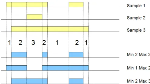
Figure 2.3: Accumulation index and COVER results with three different minAcc and

maxAccvalues.

operation is separately applied to each group, yielding to one sample in the result for each group, as discussed in Section2.3.1.

For what concerns variants:

• The_HISTOGRAM variant returns the nonoverlapping regions contribut-ing to the cover, each with its accumulation index value, which is as-signed to the AccIndex region attribute.

• The_FLATvariant returns the union of all the regions which contribute to theCOVER(more precisely, it returns the contiguous region that starts from the first end and stops at the last end of the regions which would contribute to each region of theCOVER).

• The _SUMMIT variant returns only those portions of the result regions of the COVER where the maximum number of regions intersect (more precisely, it returns regions that start from a position where the num-ber of intersecting regions is not increasing afterwards and stops at a position where either the number of intersecting regions decreases, or it violates the max accumulation index).

Example. Fig. ?? shows three applications of theCOVER operation on three samples, represented on a small portion of the genome; the figure shows the values of accumulation index and then the regions resulting from setting the minAcc andmaxAcc parameters respectively to (2, 2), (1, 2), and (2, 3).

(38)

The following COVER operation produces output regions where at least 2 and at most 3 regions of EXP overlap, having as resulting region attributes the min p-Value of the overlapping regions and their Jaccard indexes; the result has one sample for each inputCellLine.

RES = COVER(2, 3; p-Value AS MIN(p-Value) GROUP_BY CellLine) EXP

Map

<S3> = MAP [(JOINBY <Am1>, .., <Amn>)]

(<Ar1> AS <g1>, .., <Arn> AS <gn>] <S1> <S2>;

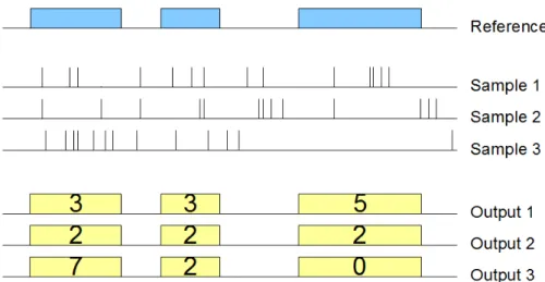
MAP is a binary operation over two datasets, respectively called reference and experiment. Let us consider one reference sample, with a set of ref-erence regions; the operation computes, for each sample in the experiment, aggregates over the values of the experiment regions that intersect with each reference region; we say that experiment regions are mapped to reference re-gions. The operation produces a matrix structure, called genomic space, where each experiment sample is associated with a row, each reference region with a column, and the matrix entries is a vector of numbers5_{. Thus, a}_MAP

operation allows a quantitative reading of experiments with respect to the reference regions; when the biological function of the reference regions is not known, the MAPhelps in extracting the most interesting regions out of many candidates.

We first consider the basic MAP operation, without JOINBY clause. For a given reference sample s1, let R1 be the set of its regions; for each

sam-ple s2 of the second operand, with s2 =< id2, R2, M2 > (according to the

GDM notation), the new sample s₃ =< id3, R3, M3 > is constructed; id3

is generated from id1 and id26, the metadata M3 are obtained by merging

metadata M1 and M2, and the regions R3 = {< c3, f3 >} are created such

that, for each region r₁ ∈ R₁, there is exactly one region r₃ ∈ R₃, having the same coordinates (i.e., c3 = c1) and having as features f3 obtained as

the concatenation of the features f₁ and the new attributes computed by the aggregate functions g specified in the operation; such aggregate functions are applied to the attributes of all the regions r2 ∈ R2 having a non-empty

5

Biologists typically consider the transposed matrix, because there are fewer exper-iments (on columns) than regions (on rows). Such matrix can be observed using heat maps, and its rows and/or columns can be clustered to show patterns.

6

The implementation generates identifiers for the result by applying hash functions to the identifiers of operands, so that resulting identifiers are unique; they are identical if generated multiple times for the same input samples.

(39)

intersection with r₁. A default aggregateCountcounts the number of regions r2 ∈ R2 having a non-empty intersection with r1. The operation is iterated

for each reference sample, and generates a sample-specific genomic space at each iteration.

When theJOINBYclause is present, for each sample s1 of the first dataset S1 we consider the regions of the samples s2 of S2 that satisfy the join condition. Syntactically, the clause consists of a list of attribute names, which are homonyms from the schemas of S1 and of S2; the stringsLEFT or RIGHT that may be present as prefixes of attribute names as result of binary operators are not considered for detecting homonyms.

Figure 2.4: Example of map using one sample as reference and three samples as exper-iment, using the Count aggregate function.

Example. Fig. ?? shows the effect of thisMAPoperation on a small portion of the genome; the input consists of one reference sample and three mutation experiment samples, the output consists of three samples with the same regions as the reference sample, whose features corresponds to the mumber of mutations which intersect with those regions. The result can be interpreted as a (3 × 3) genome space.

In the example below, the MAP operation counts how many mutations occur in known genes, where the datasetEXPcontains DNA mutation regions and GENEScontains the genes.

RES = MAP(COUNT) GENES EXP;

Join

(40)

<S1> <coord-gen> <S2>;

TheJOINoperation applies to two datasets, respectively called anchor (the first one) and experiment (the second one), and acts in two phases (each of them can be missing). In the first phase, pairs of samples which satisfy the JOINBY predicate (also called meta-join predicate) are identified; in the second phase, regions that satisfy the genometric predicate are selected. The meta-join predicate allows selecting sample pairs with appro-priate biological conditions (e.g., regarding the same cell line or antibody); syntactically, it is expressed as a list of homonym attributes from the schemes ofS1and S2, as previously. The genometric join predicate allows expressing a variety of distal conditions, needed by biologists. The anchor is used as startpoint in evaluating genometric predicates (which are not symmetric). The join result is constructed as follows:

• The meta-join predicates initially selects pairs s₁ of S1 and s₂ of S2 that satisfy the join condition. If the clause is omitted, then the Carte-sian product of all pairs s1 of S1 and s2 of S2 are selected. For each

such pair, a new sample s₁₂is generated in the result, having an identi-fier id12, generated from id1 and id2, and metadata given by the union

of metadata of s₁ and s₂.

• Then, the genometric predicate is tested for all the pairs < r_i, rj >

of regions, with r1 ∈ s1 and rj ∈ s2, by assigning the role of anchor

region, in turn, to all the regions of s1, and then evaluating the join condition with all the regions of s2. From every pair < ri, rj > that

satisfies the join condition, a new region is generated in s12.

From this description, it follows that the join operation yields to results that can grow quadratically both in the number of samples and of regions; hence, it is the most critical GMQL operation from a computational point of view. Genometric predicates are based on the genomic distance, defined as the number of bases (i.e., nucleotides) between the closest opposite ends of two regions, measured from the right end of the region with left end lower coordinate.7 A genometric predicate is a sequence of distal conditions, defined as follows:

• UP/DOWN8denotes the upstream and downstream directions of the genome. They are interpreted as predicates that must hold on the region s2 of 7_{Note that with our choice of interbase coordinates, intersecting regions have distance}

less than 0 and adjacent regions have distance equal to 0; if two regions belong to different chromosomes, their distance is undefined (and predicates based on distance fail).

(41)

the experiment;UPis true when s₂is in the upstream genome of the an-chor region9. When this clause is not present, distal conditions apply to both the directions of the genome.

• MD(K)10 denotes the minimum distance clause; it selects the K regions of the experiment at minimal distance from the anchor region. When there are ties (i.e., regions at the same distance from the anchor region), regions of the experiment are kept in the result even if they exceed the K limit.

• DLE(N)11denotes the less-equal distance clause; it selects all the regions of the experiment such that their distance from the anchor region is less than or equal to N bases12.

• DGE(N)13 denotes the greater-equal distance clause; it selects all the regions of the experiment such that their distance from the anchor region is greater than or equal to N bases.

Genometric clauses are composed by strings of distal conditions; we say that a genometric clause is well-formed iff it includes the less-equal distance clause; we expect all clauses to be well formed, possibly because the clause DLE(Max) is automatically added at the end of the string, where Max is a problem-specific maximum distance.

Example. The following strings are legal genometric predicates: DGE(500), UP, DLE(1000), MD(1)

DGE(50000), UP, DLE(100000), (S1.left - S2.left > 600) DLE(2000), MD(1), DOWN

MD(100), DLE(3000)

Note that different orderings of the same distal clauses may produce different results; this aspect has been designed in order to provide all the required biological meanings.

9

Upstream and downstream are technical terms in genomics, and they are applied to regions on the basis of their strand. For regions of the positive strand (or for unstranded regions),UPis true for those regions of the experiment whose right end is lower than the left end of the anchor, andDOWNis true for those regions of the experiment whose left end is higher than the right end of the anchor. For the negative strand, ends and disequations are exchanged.

10_{Also: MINDIST, MINDISTANCE.} 11_{Also: DIST <= N , DISTANCE <= N .}

12_{DLE(-1) is true when the region of the experiment overlaps with the anchor region;}

DLE(0) is true when the region of the experiment is adjacent to or overlapping with the anchor region.

(42)

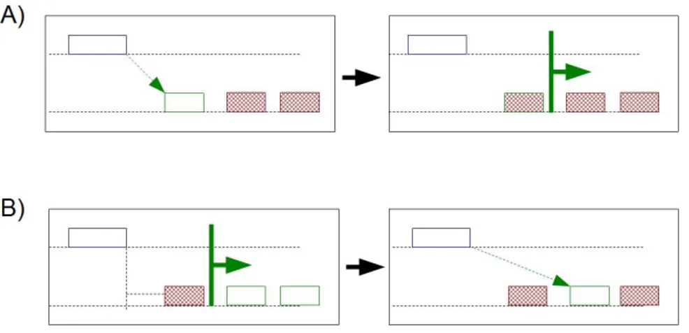
Figure 2.5: Different semantics of genometric clauses due to the ordering of distal conditions; excluded regions are gray.

Examples. In Fig. ?? we show an evaluation of the following two clauses relative to an anchor region: A: MD(1), DLE(100); B: DLE(100), MD(1). In case A, theMD(1)clause is computed first, producing one region which is next excluded by computing theDLE(100)clause; therefore, no region is produced. In case B, theDLE(100)clause is computed first, producing two regions, and then theMD(1) clause is computed, producing as result one region14.

Similarly, the clausesA: MD(1), UPandB: UP, MD(1)may produce differ-ent results, as in case A the minimum distance region is selected regardless of streams and then retained iff it belongs to the upstream of the anchor, while in case B only upstream regions are considered, and the one at minimum distance is selected.

Next, we discuss the structure of resulting samples. Assume that regions ri of si and rj of sj satisfy the genometric predicate, then a new region

rij is created, having merged features obtained by concatenating the feature

attributes of the first dataset with the feature attributes of the second dataset as discussed in Section2.3.1. The coordinates cij are generated according to

thecoord-genclause, which has four options15:

1. LEFTassigns to r_ij the coordinates c_i of the anchor region. 2. RIGHT assigns to rij the coordinates cj of the experiment region.

3. INTassigns to r_ij the coordinates of the intersection of r_iand r_j; if the

14_{The two queries can be expressed as: produce the minimum distance region iff its}

distance is less than 100 bases and produce the minimum distance region after 100 bases.

15_{If the operation applies to regions with the same strand, the result is also stranded in}

(43)

intersection is empty then no region is produced.

4. CAT (also: CONTIG) assigns to rij the coordinates of the concatenation

of r_i and r_j (i.e., the region from the lower left end between those of ri and rj to the upper right end between those of ri and rj).

Example. The following join searches for those regions of particular ChIP-seq experiments, called histone modifications (HM), that are at a minimal distance from the transcription start sites of genes (TSS), provided that such distance is greater than 120K bases16. Note that the result uses the coordinates of the experiment.

RES = JOIN(MD(1), DLE(12000); RIGHT) TSS HM;

2.3.3 Materialization of the results

Having performed a series of operations on a set of variables, at a certain point the user will have to declare that he wants to compute the resulting dataset w.r.t. a particular variable. This can be done using theMATERIALIZE operator.

MATERIALIZE <S1> INTO file_name; The result is saved in a file.

It must be noticed that all the dataset defined in GMQL are temporary in the sense that their content is not stored in memory if the corresponding variable is not materialized.

All the declarations before a MATERIALIZE operation are merely a decla-ration of intent : no opedecla-ration is performed until a materialization. This is a very important point and it will be crucial in the definition of our solution.

2.3.4 Some examples

In the following we show a set of examples demonstrating the power of the language:

Find somatic mutations in exons

We have a set of samples representing mutations in human breast cancer cases. We want to quantify how many mutation there are for each exon17

16_{This query is used in the search of enhancers, i.e., parts of the genome which have an}

important role in gene activation.

17_{An exon is a portion of a gene which will encode part of the RNA codified by that}

(44)

and select the ones that have at least one mutation. As a final step we also want to order the result, given as a set of samples, by the number of exons present in each sample.

Mut = SELECT(manually_curated|dataType == ’dnaseq’ AND

clinical_patient|tumor_tissue_site == ’breast’) HG19_TCGA_dnaseq; Exon = SELECT(annotation_type == ’exons’ AND

original_provider == ’RefSeq’) HG19_BED_ANNOTATION; Exon1 = MAP() Exon Mut;

Exon2 = SELECT(count_Exon_Mut >= 1) Exon1; Exon3 = EXTEND(exon_count AS COUNT()) Exon2; Exon_res = ORDER(exon_count DESC) Exon3; MATERIALIZE Exon_res INTO Exon_res

The first operation retrieves the mutations in which we are interested: it uses the datasetHG19_TCGA_dnaseq that provides DNA sequencing data in various cancer types and selects the ones about breast cancer. The second operation works on HG19_BED_ANNOTATION which represents the full genome annotated in significant parts and gets all the coordinates of the exons. Both these dataset are aligned to the hg19 reference genome18.

A MAPoperation follows which counts, for every exon, how many muta-tions happen to be on it. This is the most important operation in the query as it contains basically all the main logic of the program. Follows a simple selection to filter out exons having no mutations.

TheEXTEND operation is used to put in the metadata of each sample how many exons are present in it. Follows the ordering which uses the metadata exon_countjust created and puts the samples in descending order.

The query ends with a typical materialization.

Find distal bindings in transcription regulatory regions

We want to Find all enriched regions (peaks) in CTCF transcription factor (TF) ChIP-seq samples from different human cell lines which are the nearest regions farther than 100 kb from a transcription start site (TSS). For the same cell lines, find also all peaks for the H3K4me1 histone modifications (HM) which are also the nearest regions farther than 100 kb from a TSS. Then, out of the TF and HM peaks found in the same cell line, return all TF peaks that overlap with both HM peaks and known enhancer (EN) regions.

18

A reference genome is a DNA sequence database that is used by scientists to align their experiments to a common point of reference. There are several versions for different species, based on the recency and accuracy

(45)

TF = SELECT(dataType == ’ChipSeq’ AND view == ’Peaks’ AND antibody_target == ’CTCF’) HG19_ENCODE_NARROW; HM = SELECT(dataType == ’ChipSeq’ AND view == ’Peaks’

AND antibody_target == ’H3K4me1’) HG19_ENCODE_BROAD; TSS = SELECT(annotation_type == ’TSS’

AND provider == ’UCSC’) HG19_BED_ANNOTATION; EN = SELECT(annotation_type == ’enhancer’

AND provider == ’UCSC’) HG19_BED_ANNOTATION;

TF1 = JOIN(distance > 100000, mindistance(1); output: right) TSS TF; HM1 = JOIN(distance > 100000, mindistance(1); output: right) TSS HM; HM2 = JOIN(distance < 0; output: int) EN HM1;

TF_res_0 = MAP(joinby: cell) TF1 HM2;

TF_res = SELECT(count_HM2_TF1 > 0) TF_res_0; MATERIALIZE TF_res INTO TF_res;

The first four operations prepare the variables of the relative dataset for the later computation; in particular:

• We load fromHG19_ENCODE_NARROWintoTFall the samples representing peaks relative to the CTCF transcription factor.

• We load fromHG19_ENCODE_BROAD intoHM all the samples representing peaks relative to the H3K4me1 histone modification

• Using HG19_BED_ANNOTATION find all the coordinates relative to en-hancers (EN) and transcription starting site (TSS)

The first thing we do is to join the transcription starting sites to the CTCF transcription factor. We select only the CTCF which are farther than 100 kb from a TSS. Same process is done for the histone modification. Now we take only theHM1regions that intersect with an enhancerENand we take the intersection of the resulting regions intoHM2.

Finally, for each cell line, we count how many regions in HM2 intersect with the transcription factor regions in TF1and take only the transcription factors having at least oneHM2.

2.4 Architecture of the system

The architecture of the system underwent a series of revisions during time. In the initial release (see figure 2.6) [16] the GMQL queries were trans-lated to PIG [1]. Basically a translator between GMQL and Pig Latin [25]

(46)

Figure 2.6: First version of GMQL. The architecture.

was developed. Pig Latin is a language designed to act as a bridge between the declarative world of SQL and the low-level performance-driven world of Map-Reduce [10].

The second version of the system completely revised the architecture and was designed to have:

• an execution layer independent from the storage one

• the possibility to have multiple engine implementations and to choose the desired one

• the possibility to have multiple storage systems

• a set of API enabling external applications or languages to interface the engines

In figure2.7we can see a graphical representation of an high level architecture of GMQL V2 [19].

We can therefore divide the implementation of the system in the following layers:

• Access layer : the highest level of the architecture. Enables external users to interact with the system. This can happen through a web interface, a command line interface and a lower level API in Scala. • Engine abstraction: at this level the system present a series of modules

(47)

Figure 2.7: Current architecture of GMQL. Taken from [19]

the language compiler and the repository manager, which interact with a DAG scheduler, whose objective is to represent the tree structure of a query. The engines are managed by a server manager and the submission of a query is managed through a launcher manager.

• Implementations: at this level there are the operator implementations in the various engines. Currently GMQL offers an implementation in SciDB, in Spark and Flink. The Spark implementation is the most updated and stable one.

• Repository implementations: the last level manages the datasets and currently GMQL enables the user to choose between a local file system, the Hadoop HDF and the SciDB repository manager.

2.4.1 User interfaces

As we have said, GMQL currently provides the following interfaces for the final user:

• A web interface (see figure 2.9): the user can specify a textual query using both its private dataset or public ones. These dataset are stored

(48)

GMQL-Submit [-username USER] [-exec FLINK|SPARK] [-binsize BIN_SIZE] [-jobid JOB_ID] [-verbose true|false] [-outputFormat GTF|TAB]

-scriptpath /where/gmql/script/is

Description: [-username USER]

The default user is the user the application is running on $USER. [-exec FLINK|SPARK]

The execution type, Currently Spark and Flink engines are supported as platforms for executing GMQL Script.

[-binsize BIN_SIZE]

BIN_SIZE is a Long value set for Genometric Map and Genometric Join operations. Dense data needs smaller bin size. Default is 5000. [-jobid JOBID]

The default JobID is the username concatenated with a time stamp and the script file name.

[-verbose true|false]

The default will print only the INFO tags. -verbose is used to show Debug mode.

[-outputFormat GTF|TAB]

The default output format is TAB: tab delimited files in the format of BED files.

-scriptpath /where/gmql/script/is/located

Manditory parameter, select the GMQL script to execute

Figure 2.8: Command line interface for sending GMQL queries.

using the repository manager. There are also utilities for building interactively the queries and for exploring the metadata of the datasets. • A command line (see figure 2.8): a very simple interface for sending

directly the GMQL scripts to execution.

2.4.2 Scripting interfaces

At a lower level of interaction we find a Scala API that the user can use to build query programmatically. This routines enable the creation of the Di-rected Acyclic Graph (DAG), which is an abstract representation of a GMQL query.

(49)

Figure 2.9: Example of web interface usage for GMQL

The execution of the query is naturally performed locally in this case and requires the user to provide all the computational environment to execute it. For example in the following example the user is required to instantiate a Spark context to support the execution of the GMQL engine.

import it.polimi.genomics.GMQLServer.GmqlServer

import it.polimi.genomics.core.DataStructures

import it.polimi.genomics.spark.implementation._

import it.polimi.genomics.spark.implementation.loaders.BedParser._

import org.apache.spark.{SparkConf, SparkContext}

val conf = new SparkConf()

.setAppName("GMQL V2.1 Spark") .setMaster("local[*]")

.set("spark.serializer",

"org.apache.spark.serializer.KryoSerializer")

val sc:SparkContext =new SparkContext(conf)

val executor = new GMQLSparkExecutor(sc=sc)

val server = new GmqlServer(executor)

val expInput = Array("/home/V2Spark_TestFiles/Samples/exp/")

val refInput = Array("/home/V2Spark_TestFiles/Samples/ref/")

val output = "/home/V2Spark_TestFiles/Samples/out/"

//Set data parsers

val DS1: IRVariable = server READ ex_data_path USING BedParser

val DS2 = server READ REF_DS_Path USING BedScoreParser2

(50)

val ds1S: IRVariable = DS1.SELECT(

Predicate("antibody", META_OP.EQ, "CTCF"))

val DSREF = DS2.SELECT(Predicate("cell", META_OP.EQ, "genes"))

//Cover Operation

val cover: IRVariable = ds1S.COVER(CoverFlag.COVER, N(1), N(2), List(), None)

//Store Data

server setOutputPath output_path MATERIALIZE cover server.run()

We can easily see from this example that this mode of usage of the system is not as easy and user-friendly as the others.

2.4.3 Engine abstractions

A GMQL query can be represented as a graph. If we simply look at the single GMQL statements in the language we could say that a node of this graph represent one statement.

Obviously, each GMQL operation can be split in different subsections (sub-nodes) and this increase the granularity of our graph representation. The first division is surely between region nodes and metadata nodes. An additional category of nodes regards meta-grouping and meta-joining: these operations are needed to group or join samples from one or more datasets.

Metadata nodes

• ReadMD: reader of metadata files

• ReadMEMRD: reader of metadata from memory • StoreMD: materialization of metadata

• SelectMD: filtering of metadata • PurgeMD: deletion of an empty dataset

• SemiJoinMD: the semi-join condition inSELECT • ProjectMD: projection of metadata

• AggregateRD: produce a new metadata based on the aggregation of region data

(51)

• GroupMD: partitions the input data into groups and creates a new meta-data for each sample indicating the belonging group

• OrderMD: orders the samples according to a metadata value

• UnionMD: union of samples of two input metadata nodes

• CombineMD: combines two metadata nodes and produces as output the union of each pair of metadata samples

• MergeMD: union of the samples of the input node

Region nodes

• ReadRD: reader of region files

• StoreRD: materialization of region data

• PurgeRD: filters out the regions from the input that have an id that is not in a metadata node

• SelectRD: filtering of region data

• ProjectRD: projection on region data

• GroupRD: partitions the regions in disjunctive sets and only one region for each partition is returned

• OrderRD: orders the regions based on one of their attributes

• RegionCover: applies the Genometric Cover to a node

• UnionRD: puts together all the regions from the input node

• DifferenceRD: difference of two datasets. Returns only the regions of the left dataset that do not intersect with the ones of the right

• GenometricJoin: applies the Genometric Join to two nodes

• GenometricMap: applies the Genometric Map to two nodes

• MergeRD: computes the union of the region nodes and assigns new ids for avoiding collisions

(52)

Meta-grouping and Meta-joining

• GroupBy: partitions the dataset based on metadata

• JoinBy: applies the join condition to the cross product of the input metadata nodes

Example query

For a better understanding of the DAG structure let’s see how the following query would be implemented as a tree structure:

GENES = SELECT(<pm1>) ANNOTATION; PEAKS1 = SELECT(<pm2>) BED_DATA; PEAKS2 = SELECT(<pm3>) BED_DATA; FILTERED = JOIN( DLE(0) ;

antibody == antibody,

cell == cell) PEAKS1 LEFT PEAKS2; FILTERED2 = GROUP(chr,start,stop,strand) FILTERED; MAPPED = MAP(COUNT) GENES FILTERED2;

MATERIALIZE MAPPED;

In figure 2.10we can see the corresponding DAG implementation.

2.4.4 Implementations

Currently the most updated and stable implementation of the DAG operators uses Spark [2]. Each DAG node has a corresponding implementation.

Since Spark itself builds a directed acyclic graph for optimize the compu-tation we result is a second (larger) DAG after the translation of the DAG operations into Spark ones.

In this work we will only focus on the Spark implementation of GMQL and our Python API will exploit only this computational engine.

(53)

(54)

Chapter 3

Interoperability issues and

design of the library

”I love the smell of napalm in the morning.”

Apocalypse now

Before getting into the description and design of the Python library that should integrate the GMQL environment with the Python programming model we need to explore and compare these two worlds.

GMQL is written in the Scala language and its main implementation exploit the Spark big data engine for doing computations. We need therefore to understand how to integrate this language and this computing engine with Python.

In this chapter we will cover the following aspects:

1. Scala: we will describe the Scala language with a particular attention on its differences with respect to Java.

2. Python: a description of the Python programming language will follow. Also the main users and usages of this language will be explained.

3. Interoperability: we will show how make a Python and a Scala program interact. This step is fundamental for the design of the PyGMQL library.

4. Interactive computation: we will show the main issues that arise when we try to make a big data computation system interactive and how this requirement was satisfied in the design of PyGMQL

(55)

Figure 3.1: Process of compilation of a Scala program

5. Alternative architectures: the last part of the chapter is dedicated to the description of the various alternative architectures that were con-sidered for PyGMQL. Advantages and disadvantages of each of them will be presented.

3.1 Scala language

Scala is a multi-paradigm programming language: it is object-oriented, im-perative and functional. Its design started in 2001 at the École Polytechnique Fédérale de Lausanne (EPFL) by Martin Odersky and it was the continu-ation of the work on Funnel, a programming language mixing functional programming with Petri nets [22]. It was publicly released in 2004 on the Java platform.

3.1.1 Compatibility with Java

Scala is implemented over the Java virtual machine (JVM) and therefore is compatible with existing Java programs [23]. The Scala compiler (scalac) generates a byte code very similar to the one generated by the Java compiler. From the point of view of the JVM the Scala byte code and the Java one are indistinguishable. In figure 3.1we can see the process of Scala compilation.

3.1.2 Extensions with respect to Java

Scala introduces a lot of syntactic and model differences with respect to Java. Follows a brief list of the main differences: