ALMA
MATER
STUDIORUM
· U
NIVERSITÀ DIBOLOGNA
SCUOLA DI SCIENZE
Corso di Laurea Magistrale in Matematica
ORTHOGONAL GAMMA-BASED
EXPANSIONS FOR VOLATILITY
OPTION PRICES UNDER
JUMP-DIFFUSION DYNAMICS
Tesi di Laurea in Finanza Quantitativa
Relatore: Chiar.mo Prof. ANDREA PASCUCCI Presentata da: ALICE BUCCIOLI Correlatrice: Chiar.ma Prof.ssa ELISA NICOLATO I I Sessione Anno Accademico 2013/2014
“DI COSTUI ALMENO IO SONO PIÚ SAPIENTE; PUÓ BEN DARSI CHE NÉ LUI NÉ IO SAPPIAMO NIENTE DI BELLO E BUONO, MA EGLI CREDE DI SAPERE NON SAPENDO, IO INVECE NON SO,E NON CREDO DI SAPERE; PARE DUNQUE CHE,ANCHE PER QUESTA PICCOLA COSA, IO SIA PIÚ SAPIENTE DI COSTUI, PERCHÉ NON RITENGO DI SAPERE QUELLO CHE NON SO. ”
P
REFACE
In this work we derive closed-form pricing formulas for vanilla options on the CBOE VIX Index by suitably approximating the volatility process risk-neutral density function. We ex-ploit and adapt the idea, which stands behind popular techniques already employed in the context of equity options such as Edgeworth or Gram-Charlier expansions, of approximating the underlying process by an alternate (and more tractable) distribution in terms of a series expansion. Jarrow and Rudd (1982) pioneered the density expansion approach to option pric-ing, deriving an option pricing formula from an Edgeworth series expansion of the log-normal probability density function to model the distribution of stock prices. Corrado and Su (1996) adopted the Jarrow-Rudd framework and derived a similar option pricing formula where the chief difference is that they employed a Gram-Charlier series expansion of the normal proba-bility density function to model the distribution of stock log prices. A probaproba-bility density func-tion f can be represented as a Gram-Charlier series expansion in the following form:
f (x) =
+∞ X k=0
ckHk(x)z(x)
where z(x) is the normal density function, Hk(x) are Hermite polynomials of order k and the coefficients ck are simple functions of the moments of the approximated distribution. More recently, Drimus, Necula and Farkas (2013) developed a new option pricing formula by em-bracing the Corrado and Su framework and employing a modified Gram-Charlier type A series expansion, replacing the “probabilists” Hermite polynomials by the “physicists” Hermite poly-nomials. These methodologies represent a valid alternative to the numerical integration tech-niques to obtain an option price in case the distribution function is not analytically tractable, but it may however be straightforward to estimate its moments. The aim of this thesis is to modestly generalize these techniques to be adapted to the context of volatility options. Indeed the expansions above-mentioned, which are successful in the context of equities, are not ap-propriate for approximating volatility densities as their support lies in the whole real line. Thus we propose an expansion based on a class of polynomials which are weighted by a Gamma dis-tribution, instead of log-normal or Gaussian distributions, thus ensuring positive mass only in the positive real line: the polynomials in question are the Laguerre polynomials. We call this series expansion Gamma-Laguerre expansion and we write
f (x) =
+∞ X k=0
ckLk(x)φ(x)
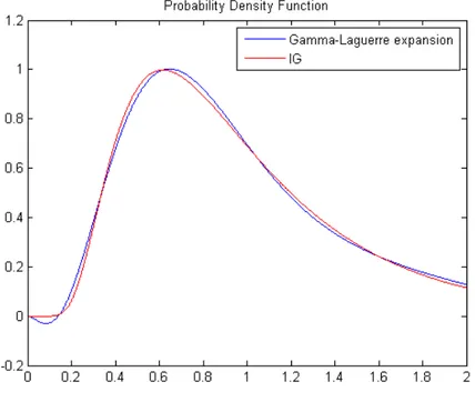
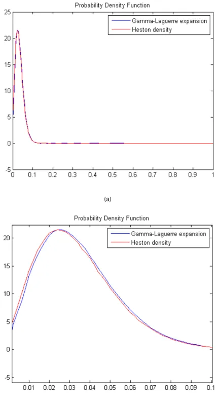
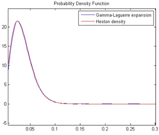
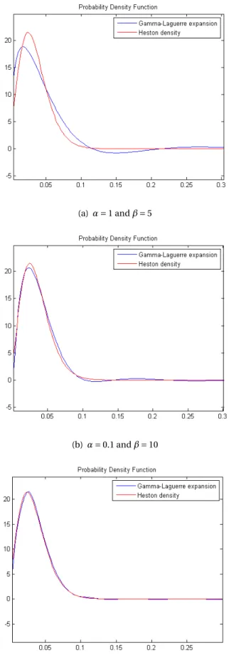
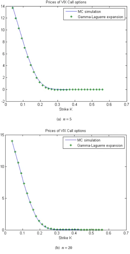
whereφ(x) denotes the Gamma density function, Lk(x) are Laguerre polynomials of order k and the coefficients ck are now expressed in function of the characteristic function of the ap-proximated volatility process risk-neutral distribution. The latter coefficients property more-over makes our “approximation recipe” an alternative procedure to the classic inverse Fourier transform methodology. The accuracy of this approximation is tested for the Heston model and
iv
closed-form pricing formulas for vanilla options on the VIX Index are developed for the Hes-ton model as well as for the jump-diffusion SVJJ model, proposed by Duffie et al. (2000). Due to the empirical evidence that prices essentially move by jumps, manifesting a discontinuous behaviour, it is of interest to look at jump-diffusion models, such as the SVJJ model where both the stock and the variance are Lévy processes. Indeed, while diffusion models cannot generate sudden, discontinuous moves in prices, jump-diffusion models overlay continuous asset price changes with jumps.
At the beginning of any chapter there is a very short introduction about the topics analyzed therein. Here we want to give the outline of the thesis.
In Chapter 1 we review some of the main results on the risk-neutral derivative valuation frame-work for continuous-time diffusion models. We show that, under this frameframe-work, the concept of Equivalent Martingale Measure Q is an essential ingredient for valuation. Indeed the value of a financial derivative corresponds, in mathematical terms, to the computation of the expected value, under the risk-neutral measure Q, of the payoff, discounted at the risk-free interest rate.
Chapter 2 is devoted to the study of the class of Affine-Jump-Diffusion processes. We turn
to-wards applications of affine processes to the modeling of stochastic volatility, by presenting two standard examples given by the Heston model and the SVJJ model. Finally, we derive explicit expressions for the characteristic function under both the above-mentioned models.
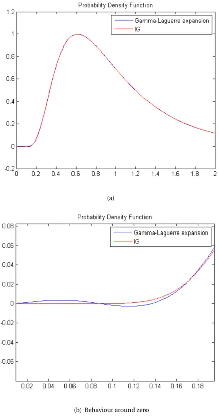
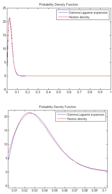
In Chapter 3 we provide the definition of the CBOE VIX Index, from both the economical and mathematical point of view. Once we have translated the VIX Index in probabilistic terms, we provide shorthand forms for the VIX squared under the Heston model as well as the SVJJ model. In Chapter 4 we describe in detail our approximation methodology, the Gamma-Laguerre
ex-pansion, and we provide some illustrative examples, based on the Inverse Gaussian
distribu-tion and the (simulated) Heston model distribudistribu-tion, to highlight the convergence of this ex-pansion.
In Chapter 5 we give a brief exposition of the contracts on the VIX Index and we derive interest-ing closed-form formulas for pricinterest-ing them under the Heston model as well as the SVJJ model.
Chapter 6 contains the numerical tests of the pricing formulas provided in Chapter 5, based on
the Heston model.
Finally, the Appendix gathers some classical results in stochastic calculus and Lévy process the-ory we consider relevant background material to the drafting of this thesis.
P
REFAZIONE
In questo lavoro ricaviamo formule di prezzo per opzioni vanilla sull’indice CBOE VIX in forma chiusa, approssimando opportunamente la funzione di densità neutrale al rischio del processo di volatilià. Utilizziamo e adattiamo l’idea che risiede dietro popolari tecniche, già impiegate nel contesto di opzioni sulle equity, come le espansioni di Edgeworth o di Gram-Charlier, di approssimare il processo sottostante con una distribuzione alternativa (e più tratta-bile) in termini di sviluppo in serie. Jarrow and Rudd (1982) hanno aperto la strada all’approccio basato su espansioni di densità per prezzare opzioni, derivando una formula di prezzo da una espansione in serie di Edgeworth della funzione di probabilità log-normale per modellare la distribuzione dei prezzi stock. Corrado and Su (1996) hanno adottato il quadro presentato da Jarrow e Rudd e derivato una simile formula di prezzo dove la principale differenza risiede nell’aver utilizzato uno sviluppo in serie di Gram-Charlier della densità di probabilità normale per modellare la distribuzione dei rendimenti logaritmici. Una funzione di densità di proba-bilità f può essere rappresentata come uno sviluppo in serie di Gram-Charlier nella seguente forma f (x) = +∞ X k=0 ckHk(x)z(x)
dove z(x) è la funzione di densità normale, Hk(x) sono i polinomi di Hermite di ordinek e i coefficienti ck sono semplici funzioni dei momenti della distribuzione approssimata. Più re-centemente, Drimus, Necula and Farkas (2013) hanno sviluppato una nuova formula di prezzo abbracciando il contesto di Corrado e Su e utilizzando uno sviluppo in serie di Gram-Charlier di tipo A modificato, sostituendo i polinomi di Hermite “probabilistici” con i polinomi di Hermite “fisici”. Queste metodologie rappresentano una valida alternativa alle tecniche di integrazione numerica usate per ottenere prezzi qualora la distribuzione non sia trattabile analiticamente, ma comunque risulti semplice valutare i suoi momenti. Lo scopo di questa tesi è di generaliz-zare, modestamente, queste tecniche cosicché possano essere adattate al contesto di opzioni sulla volatilità. Infatti le espansioni di cui sopra, che sono soddisfacenti nel contesto di equity, non sono appropriate per approssimare densità di volatilità in quanto supportate sull’intera linea reale. Proponiamo pertanto un’espansione basata su una classe di polinomi pesati da una distribuzione Gamma, anziché distribuzioni Gaussiane o log-normali, assicurando in questo modo massa positiva solo sulla linea reale positiva: i polinomi in questione sono i polinomi di Laguerre. Chiamiamo tale sviluppo in serie Espansione Gamma-Laguerre e scriviamo
f (x) =
+∞ X k=0
ckLk(x)φ(x)
doveφ(x) denota la funzione di densità Gamma, Lk(x) sono polinomi di Laguerre di ordine
k and i coefficienti ck sono ora espressi in funzione della funzione caratteristica della
dis-tribuzione neutrale al rischio del processo di volatilità che stiamo approssimando. Quest’ultima proprietà riguardante i coefficienti dell’espansione inoltre rende la nostra “ricetta” di
approssi-vi
mazione una procedura alternativa alla classica metodologia basata sulla inversione della trasfor-mata di Fourier. L’accuratezza della suddetta approssimazione è testata sul modello a volatil-ità stocastica di Heston e formule di prezzo in forma chiusa sono sviluppate sia per il mod-ello di Heston che per il modmod-ello diffusivo con salti, chiamato SVJJ, proposto da Duffie et al. (2000). Data l’evidenza empirica che i prezzi si muovono sostanzialmente con salti, manifes-tando un comportamento discontinuo, abbiamo trovato interessante anche trattare modelli di diffusione con salti, come il modello SVJJ nel quale sia il sottostante che la sua volatilità sono processi di Lévy. Infatti, mentre i modelli puramente diffusivi non possono generare repentini, discontinui movimenti nei prezzi, i modelli diffusivi con salti sovrappongono continui cambi-amenti di prezzi con salti.
All’inizio di ogni capitolo si trova una breve introduzione circa gli argomenti ivi analizzati. Qui vogliamo fornire lo schema generale della tesi.
Nel Capitolo 1 esaminiamo alcuni fra i risultati principali della teoria di valutazione neutrale al rischio di strumenti derivati in modelli a tempo continuo. Mostriamo come, in questo contesto, il concetto di Misura Martingala Equivalente Q sia un ingrediente essenziale per la valutazione. Infatti, il valore di un derivato finanziario corrisponde, in termini matematici, al calcolo del valore atteso, rispetto alla misura neutrale al rischio Q, del payoff, scontato al tasso di interesse privo di rischio.
Il Capitolo 2 è dedicato allo studio della classe di processi di salto diffusivi affini. Ci spostiamo verso le applicazioni dei processi affini nella modellizzazione di volatilità stocastiche, presen-tando due esempi classici dati dal modello di Heston e dal modello SVJJ. Infine, deriviamo epressioni esplicite per la funzione caratteristica in entrambi i suddetti modelli a volatilità sto-castica.
All’interno del Capitolo 3 forniamo la defizione di Indice CBOE VIX, sia dal punto di vista eco-nomico che dal punto di vista matematico. Dopo aver tradotto l’indice VIX in termini proba-bilistici, forniamo forme abbreviate per il quadrato del VIX sia nel modello di Heston che nel modello SVJJ.
Nel Capitolo 4 descriviamo dettagliatamente la nostra metodologia di approsimazione, l’
es-pansione Gamma-Laguerre, e forniamo qualche esempio illustrativo, basato sulla distribuzione
Inverse-Gamma e sulla distribuzione del modello di Heston (simulata), per sottolineare la con-vergenza della suddetta espansione.
All’interno del Capitolo 5 forniamo una breve descrizione circa le opzioni sull’indice VIX e de-riviamo formule in forma chiusa per valutarle, considerando sia il modello d Heston che il mod-ello SVJJ.
Il Capitolo 6 contiene i test numerici delle formule di prezzo fornire nel precedente Capitolo 5,
basate sul modello di Heston.
Infine, l’Appendice raccoglie alcuni classici risultati di calcolo stocastico e analisi di processi di Lévy che consideriamo materiale di supporto alla stesura di questa tesi.
C
ONTENTS
Preface viii
1 Risk-neutral pricing and martingale measures 1
1.1 Model assumptions. . . 1
1.2 Change of measure . . . 2
1.3 Martingale measures . . . 4
1.4 Admissible strategies and arbitrage opportunities . . . 5
1.5 Arbitrage pricing . . . 6
2 Affine Jump-Diffusion processes 9 2.1 Two standard models . . . 10
2.1.1 Heston model . . . 10
2.1.2 SVJJ model . . . 12
3 The CBOE Volatility Index - VIX 17 3.1 The VIX calculation step-by-step . . . 17
3.2 VIX Squared and Forward Price of Integrated Variance . . . 24
3.3 VIX under Heston model. . . 30
3.4 VIX under SVJJ model . . . 33
4 Gamma-Laguerre expansions 37 4.1 The Gamma choice . . . 39
4.1.1 Applications . . . 43
4.2 Laguerre-Gamma expansion coefficients . . . 48
4.2.1 Heston model . . . 49
4.2.2 SVJJ model . . . 49
5 Pricing VIX Options 51 5.1 Option contracts on the VIX . . . 51
5.2 Princing formulas . . . 52
5.2.1 Heston model . . . 54
5.2.2 SVJJ model . . . 56
6 Numerical results 59 A Appendix 69 A.1 ...regarding stochastic calculus . . . 69
A.1.1 Correlated Brownian motion . . . 70
A.1.2 Itô calculus. . . 71
A.1.3 Feynman-Kac formula . . . 72
A.2 Lévy processes. . . 73
A.2.1 Some examples of Lévy processes . . . 75
A.3 Stochastic calculus for jump-diffusion processes . . . 80
A.3.1 Itô formula for jump-diffusion processes . . . 80
A.3.2 Feynman-Kac representation . . . 82
1
R
ISK
-
NEUTRAL PRICING AND
MARTINGALE MEASURES
Two important concepts in the mathematical theory of option pricing are the absence of
arbi-trage, which imposes constraints on the way instruments are priced in a market and the notion
of risk-neutral price, which represents the price of any derivative in an arbitrage-free market as its discounted expected payoff at the risk-free interest rate under an appropriate probability measure called the “risk-neutral” measure. Both of these notions are expressed in mathemati-cal terms exploiting the concept of Equivalent Martingale Measure (EMM) which plays, in this chapter, a central role: in a market model defined by a probability measure P on market sce-narios there is a one-to-one correspondence between risk-neutral pricing that avoids the in-troduction of arbitrage opportunities and risk-neutral probability measure Q, equivalent to P verifying a martingale property. Since this chapter is intended as an introduction for the theory of derivative pricing for continuous-time diffusion models, the proofs of the results we state are omitted: for a complete treatment of the theory we refer to [15].
1.1 Model assumptions
First of all, we set the assumptions on the model that are going to hold in the rest of the chapter. Thus, we consider a market whose possible evolutions between 0 and T are described by a probability spaceP:= (Ω,F, P ) and consisting of N risky assets, one non-risky asset and
d sources of risk that are represented by a d −dimensional correlated Brownian motion W =
¡W1
, ··· ,Wd¢ on the probability spacePendowed with the Brownian filtrationFWt =¡FWt ¢
2 1. Risk-neutral pricing and martingale measures
1.
Underlying assets may then be described by a stochastic process:
S : [0, T ] × Ω −→ RN
(t ,ω) −→ ¡S1t(ω),··· ,SNt (ω)¢
where Sit(ω) represents the price of the risky asset i at time t in the market scenario ω whose dynamics is given by
d Sit= µitSitd t + σitSitdWti, i = 1,··· , N , t ∈ [0,T ]
withµi∈ L1locandσi∈ L2loc. Concerning the non-risky asset B , we suppose it is a cash account with fixed (risk-free) interest rate r fulfilling the following formula of continuous compounding
Bt= er t, B0= 1, t ∈ [0,T ]
or, equivalently, in the “differential form”
d Bt= r Btd t .
Before going any further, it is good to briefly recall some notions about derivative instruments. Discounting is done using the numeraire Bt: indeed, for any portfolio with value Vt, the
dis-counted value is defined by
˜
Vt=
Vt
Bt .
An option with maturity T may be represented by specifying its terminal payoff H (ω) in each scenario: since H is revealed at T , the payoff is aFT−measurable map
H :Ω −→ R.
1.2 Change of measure
Definition 1.1. Letλ ∈ L2locbe a d −dimensional process. We call exponential martingale
asso-ciated toλ the process
Ztλ= exp µ − Z t 0 λs· dWs− 1 2 Z t 0 |λs| 2d s ¶ , t ∈ [0,T ].
1The natural filtration for W is defined by
˜ FW
t = σ (Ws|0 ≤ s ≤ t ) := σ
³n
Ws−1(B )|0 ≤ s ≤ t, B ∈Bo´, t ∈ [0,T ]. We call Brownian filtration, and we denote it byFWt =¡FWt
¢
t ∈[0,T ], the filtration defined as the natural filtration
completed by the collection of P -negligible events, i.e.
FW
t = σ³ ˜FWt ∪N
´
whereN=©F ∈F|P (F ) = 0ª. The choice of considering the filtration containing negligible events stems from the need of avoiding the unpleasant situation in which W1= W2a.s., W1isFt-measurable but W2fails to be so.
1.2 Change of measure 3
Remark 1.2. The exponential martingale associated toλ can be written in the “differential form” as follows
d Xtλ:= d ln(Zt)λ= −λtdWt− 1 2|λt|
2d t
whence, by employing the Itô formulaA.2to the process f (Xtλ) = eXtλ= Zλ
t , we get d Ztλ= d f = eXtλd Xλ t + 1 2|λt| 2eXtλd t = eXtλ(−λt· dWt−1 2|λt| 2 d t ) +1 2|λt| 2eXtλd t = −Ztλλt· dWt.
Therefore Zλis a local martingale.
The following central theorem shows that it is possible to substitute “arbitrarily” the drift of an Itô process by modifying properly the considered probability measure and Brownian mo-tion, while keeping unchanged the diffusion coefficient.
THEOREM - 1.2.1 (Girsanov’s theorem).
Let Zλbe the exponential martingale associated to the processλ ∈ L2loc. We assume that Zλis a
P −martingale and we consider the measure Q defined by dQ
d P = Z
λ T.
Then the process
Wtλ= Wt+ Z t
0 λs
d s, t ∈ [0,T ], is a Brownian motion on (Ω,F,Q, (Ft)).
THEOREM - 1.2.2 (Change of drift).
Let Q be a probability measure equivalent to P . The Radon-Nikodym derivative of Q with respect to P is an exponential martingale dQ d P ¯ ¯ ¯ FW t = Ztλ, d Ztλ= −Ztλλt· dWt
withλ ∈ L2locand the process Wλ, defined by
dWt= dWtλ− λtd t ,
is a Brownian motion on (Ω,F,Q, (FWt )).
We now extend the previous result to the case of the correlated Brownian motion. THEOREM - 1.2.3 (Change of drift with correlation).
If Q is a probability measure equivalent to P then there exists a processλ ∈ L2locsuch that dQ d P ¯ ¯ ¯ FW t = Ztλ, d Ztλ= −Ztλλt· dWt.
Moreover, the process Wλ, defined by
dWt= dWtλ− ρλtd t ,
4 1. Risk-neutral pricing and martingale measures
Remark 1.3. Under the assumptions of Theorem1.2.3, let X be an N -dimensional Itô process of the form
d Xt= btd t + σtdWt. Then the Q−dynamics of X is given by
d Xt= (bt− σtρλt)d t + σtdWtλ.
Again, we emphasize the fundamental feature of the change of measure: it only affects the drift coefficient of the process X, whilst the diffusion coefficient (or volatility) does not vary.
1.3 Martingale measures
Definition 1.4. An Equivalent Martingale Measure (EMM) Q with numeraire B is a probability measure on (Ω,P) such that
(i) Q is equivalent to P, i.e.
P ∼ Q ⇐⇒ ∀A ∈F, P (A) = 0 ⇔ Q(A) = 0
namely that P and Q define the same set of (im)possible events. (ii) The process of discounted prices
˜
St= e−r tSt, t ∈ [0,T ]
is a Q−martingale. Therefore, in particular, the risk-neutral pricing formula
St= e−r (T −t )EQ£ST|FWt ¤ holds.
Now we consider an EMM Q and we use Theorem1.2.3, in the form of Remark1.3, to find the
Q−dynamics of the price process. We recall that there exists a process λ = (λ1, ··· ,λd) ∈ L2loc
such that dQ d P ¯ ¯ ¯ FW t = Zt where d Zt= −Zt(ρ−1λt) · dWt, Z0= 1. (1.1) Moreover the process Wλ= (Wλ,1, ··· ,Wλ,d) defined by
dWt= dWtλ− λtd t
is a Q−Brownian motion with correlation matrix ρ. Therefore, for i = 1,··· , N , we have
d ˜Sit= (µit− rt) ˜Sitd t + σ i tS˜itdW i t = (µit− rt) ˜Sitd t + σ i tS˜it(dWtλ,i− λ i td t ) = (µit− rt− σitλit) ˜Sitd t + σitS˜itdWtλ,i.
1.4 Admissible strategies and arbitrage opportunities 5
Now we recall that an Itô process is a local martingale if and only if it has null drift (cf. Remark
A.6). Therefore, since Q is an EMM, the following drift condition necessarily holds:
λi t= µi t− rt σi t , i = 1,··· , N . (1.2)
Finally we give the following
Definition 1.5. A market price of risk is a d −dimensional process λ ∈ L2locsuch that: (i) the first N components ofλ are given by (1.2);
(ii) the solution Z to the SDE (1.1) is a strict P −martingale.
1.4 Admissible strategies and arbitrage opportunities
Definition 1.6. A strategy (or portfolio) is a stochastic process inRN +1 (α,β) = ¡α1t, ··· ,αNt ,βt¢ , t ∈ [0,T ]
such thatα,β ∈ L1loc. In financial terms,αit(resp.βt) represents the amount of the asset Si(resp. bond) held in the portfolio at time t . The value of the portfolio (α,β) is the real-valued process
Vt(α,β)= αt· St+ βtBt= N X i =1 αi tSit+ βtBt, t ∈ [0,T ]. Definition 1.7. A strategy (α,β) is self-financing if
dVt= αt· dSt+ βtd Bt. (1.3)
From a purely intuitive point of view, (1.3) expresses the fact that the instantaneous variation of the value of the portfolio is caused uniquely by the changes of the prices of the assets, and not by injecting or withdrawing funds from outside. Therefore, in a self-financing strategy we establish the wealth we want to invest at the initial time and afterwards we do not inject or withdraw funds.
Proposition 1.4.1. Let Q be an EMM and (α,β) a self-financing strategy such that
αiσi
∈ L2loc(Ω,P), i = 1,··· ,N (1.4)
then, ˜Vt(α,β)is a Q−martingale. Therefore, in particular, the following risk-neutral pricing for-mula
Vt(α,β)= e−r (T −t )EQhVT(α,β)|FWt i
, t ∈ [0,T ] holds.
Definition 1.8. A self-financing strategy (α,β) such that ˜V(α,β) is a Q−martingale for every EMM Q, is called an admissible strategy. We denote byAthe collection of all admissible strate-gies.
Proposition1.4.1 guarantees that the familyAis not empty: indeed, any self-financing strategy (α,β) verifying condition (1.4) is admissible. Moreover we have the following version of the no-arbitrage principle.
6 1. Risk-neutral pricing and martingale measures
Proposition 1.4.2 (No-arbitrage principle).
If an EMM exists and (α,β), (α0,β0) are admissible self-financing strategies such that
VT(α,β)= VT(α0,β0) P − a.s. then V(α,β)and V(α0,β0)are indistinguishable.
Proof. If Q exists and (α,β), (α0,β0) are admissible, then ˜V(α,β)and ˜V(α0,β0)
are Q−martingales with the same final value Q−a.s., because Q ∼ P. Hence
˜ Vt(α,β)= EQhV˜T(α,β)¯¯ ¯Ft i = EQhV˜T(α0,β0)¯¯ ¯Ft i = ˜Vt(α0,β0) for every t ∈ [0,T ].
1.5 Arbitrage pricing
We now analize the problem of pricing of a European derivative.
Definition 1.9. A derivative X is called replicable if there is an admissible strategy (α,β) ∈A such that
X = VT(α,β) P − a.s. (1.5)
where the random variable X represents the payoff of the derivative. An admissible strategy (α,β) such that (1.5) holds, is called a replicating strategy for X.
Definition 1.10. The risk-neutral price of a European derivative X with respect to the EMM Q, is defined as
HQt = e−r (T −t )EQ£X |FW
t ¤ , t ∈ [0,T ].
Next we introduce the collections of super and sub-replicating strategies: A+ X = n (α,β) ∈A|VT(α,β)≥ X , P − a.s. o A− X = n (α,β) ∈A|VT(α,β)≤ X , P − a.s.o
For a given (α,β) ∈A+X(resp. (α,β) ∈A−X), the value V0(α,β)represents the initial wealth sufficient to build a strategy that super-replicates (resp. sub-replicates) the payoff X at maturity. The following result confirms the natural consistency relation among the initial values of the sub and super-replicating strategies and the risk-neutral price: this relation must necessarily hold true in any arbitrage-free market, otherwise arbitrage opportunities could be easily created. Lemma 1.5.1. Let X be a European derivative. For every EMM Q and t ∈ [0,T ] we have
sup (α,β)∈A− X Vt(α,β)≤ e−r (T −t )EQ£X |FW t ¤ ≤ inf (α,β)∈A+ X Vt(α,β).
Lemma1.5.1ensures that any risk-neutral price does not give rise to arbitrage opportuni-ties since it is greater than the price of every sub-replicating strategy and smaller than the price of every super-replicating strategy. By definition, HQdepends on the selected EMM Q; how-ever, this is not the case if X is replicable. Indeed the following result shows that the risk-neutral price of a replicable derivative is uniquely defined and independent of Q.
1.5 Arbitrage pricing 7
THEOREM - 1.5.2. Let X be a replicable European derivative. For every replicating strategy
(α,β) ∈Aand for every EMM Q, we have
Ht:= Vt(α,β)= e−r (T −t )EQ£X |FWt ¤ .
The process H is called risk-neutral (or arbitrage) price of X.
The following result shows that, if the number of risky assets is equal to the dimension of the underlying Brownian motion, i.e. N = d, then the market is complete and the martingale measure is unique. Roughly speaking, in a complete market every European derivative X is replicable and by Theorem1.5.2it can be priced in a unique way by arbitrage arguments: the price of X coincides with the value of any replicating strategy and with the risk-neutral price under the unique EMM.
THEOREM - 1.5.3. When N = d, the market model (S,B) is complete, that is every European
derivative is replicable. Moreover there exists only one EMM.
Example 1.11 (Heston model).
Heston [8] proposed the following stochastic volatility model:
d St= µStd t +pvtStdWt(1) (1.6)
d vt= k( ¯v − vt)d t + ²pvtdWt(2) (1.7) where {St}t ≥0, {vt}t ≥0are the price and volatility processes, respectively, andnWt(1)o
t ≥0, n
Wt(2)o
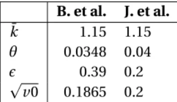
t ≥0 are correlated Brownian motion processes (with correlation parameterρ). {vt}t ≥0is a square root mean reverting process, previously suggested by Cox, Ingersoll and Ross (1985) as a model for the short rate dynamics in a fixed-income market, with long-run mean ¯v, and rate of
rever-sion k. ² is referred to as the volatility of volatility. All the parameters, namely µ,k, ¯v,²,ρ, are time and state homogenous. Finally, the interest rate r is supposed to be constant. By the Itô formulaA.2, the solution of (1.6) is
St= S0exp µZ t 0 p vsdWt(1)+ Z t 0 ³ µ −vs 2 ´ d s ¶ .
A market price of risk is a two-dimensional processλ = (λ(1),λ(2)) ∈ L2locsuch that
λ(1) t =
µ − r
p
vt
while there is no restriction on the second componentλ(2)except for the fact that Z must be a martingale. If this is the case, we consider the corresponding EMM Q with respect to which the process Wλ, defined by dWt= dWtλ− λtd t = dWtλ− Ã µ−r pv t λ(2) t ! d t ,
is a two-dimensional Brownian motion. Thus the Q−dynamics are given by
d St= r Std t +pvtStdWt(S) (1.8) d vt= ³ k( ¯v − vt) − ²pvtλ(2)t ´ d t + ²pvtdWt(v)
8 1. Risk-neutral pricing and martingale measures
where dWt(S):= dWtλ,(1)and dWt(v)= dWtλ,(2). We remark that by taking the processλ(2)of the form λ(2) t = avt+ b p vt
with some real constants a, b, the Q−dynamics of the volatility process reduces to
d vt= ¯k(θ − vt)d t + ²pvtdWt(v) (1.9)
where
¯
k := k + ²a, θ :=k ¯v − ²b k + ²a
and therefore v is a square root process under Q as well.
We note that while the drift in (1.8) must be r under any EMM with the cash account as nu-meraire, we could use Girsanov’s Theorem to change the drift in (1.9) in infinitely many dif-ferent ways without changing the drift in (1.8). This means that the EMM is not unique, there are infinitely many EMM’s depending on the value ofλ(2), thus, in view of Theorem1.5.3, the Heston stochastic volatility model is an incomplete model. This should not be too surprising as there are two sources of uncertainty in the Heston model, W(S)and W(v), but only one risky asset and so not every security is replicable. The implications are that the different EMM’s will produce different option prices, depending on the value ofλ(2): this, initially, poses a problem but we remark that from the economical point of view, the price of riskλ is determined by the market, namely,λ must be chosen on the basis of observations, by calibrating the parameters of the model to the available data. Therefore, onceλ and the corresponding EMM Q have been selected, the risk neutral price of a derivative on S is defined as in Definition1.10.
2
A
FFINE
J
UMP
-D
IFFUSION PROCESSES
In this chapter we present Affine-Jump-Diffusion (AJD) processes and the Fourier transform calculation that will later be useful in option pricing. This class consists of all jump-diffusion processes, whose drift vector, covariance matrix and arrival rate of jumps all depend in an affine way on the state process. The attractiveness of affine processes for Finance stems from sev-eral reasons: firstly, a variety of models that have been proposed in the literature, and that are used by practitioners, fall into the class of affine models. For instance, in the area of interest rate models, prominent among affine models are the classical models of Vasicek [1977] and Cox, Ingersoll, and Ross [1985]; in the realm of asset price modelling, the Black-Scholes model, all exponential-Lévy models (cf. [3]), the model of Heston [1993], extensions of the Heston model, such as Bates [1996] and Bates [2000] are all based on affine processes. Secondly, affine processes exhibit a high degree of analytic tractability: the computation of the characteristic function can be reduced to a system of Riccati equations, which have in many cases explicit solutions. The explicit knowledge of the Fourier transform allows an analytical treatment of a range of valuation problems: Fourier inversion methods can be employed as well as alternative techniques, based on Fourier transform, such as the methodology provided by this work. Let (Ω,F, P ) be a probability space endowed with an information filtration (Ft). Suppose that
X = (Xt)t ∈[0,T ]is anFt-adapted continuous process solving the stochastic differential equation
d Xt= µ(t , Xt)d t + σ(t, Xt)dWt+ d Zt (2.1) where
• W is a d −dimensional Brownian motion on the filtered probability space (Ω,F, P, (Ft)) • µ = µ(t,x) : [0,T ] × Rn−→ Rnis the drift coefficient,µ(t, Xt) ∈ L1loc
• σ = σ(t,x) : [0,T ] × Rn−→ Rn×dis the diffusion coefficient,σ(t, Xt) ∈ L2loc
• Z is a pure jump process whose jumps have a fixed probability distribution m and arrive with intensityλ.
10 2. Affine Jump-Diffusion processes
Definition 2.1. We call Affine-Jump-Diffusion (AJD) process the stochastic process X = (Xt)t ∈[0,T ] satisfying (2.1) such that the parameter functions µ,σ and λ are determined by coefficients (K , H , l ) defined as follows:
• µ(t,x) = K0+ K1· x, for K := (K0, K1) ∈ Rn× Rn×n
• ¡σ(x)σ(x)T¢i j= (H0)i j+ (H1)i j· x, for H := (H0, H1) ∈ Rn×n× Rn×n×n • λ(x) = l0+ l1· x, for l := (l0, l1) ∈ R × Rn.
2.1 Two standard models
In this section we will look more closely at the most common affine one factor models, restrict-ing our attention to the derivation of a closed-form expression for the Fourier transform.
2.1.1 Heston model
In the Heston stochastic volatility model, the risk-neutral dynamics for the joint process (S, v) is given by
(
d St= r Std t +pvtStdWt(S)
d vt= ¯k(θ − vt)d t + ²pvtdWt(v)
(2.2)
where W :=¡W(S),W(v)¢ is a two-dimensional correlated Brownian motion, with correlation parameterρ, the constant parameters ¯k,θ are responsible for a mean-reverting ability of the process and² is volatility of volatility vt. To ensure that the process v is strictly positive, the parameters must obey the following condition
2 ¯kθ > ²2 (2.3)
known as the Feller condition. Furthermore, we assume that both the stochastic processes (pvt)tand (Stpvt)tbelong to the classL2.
Starting from the dynamics (2.2) of the asset, by the Itô formulaA.2, we can easily compute the equivalent risk-neutral dynamics for the joint process (ln(S), v)
(
d ln(St) =¡r −v2t¢ d t +pvtdWt(S)
d vt= ¯k(θ − vt)d t + ²pvtdWt(v).
(2.4)
Furthermore, we shall prove that the discounted asset fulfills the martingale property: indeed, by applying the Itô lemma to f (t , St) = e−r tSt, we get
d f = −r e−r tStd t + e−r td St
= −r e−r tStd t + e−r tr Std t + e−r tpvtStdWt(S) = e−r tpvtStdWt(S)
which corresponds to the following SDE:
e−r tSt= S0+ Z t
0 e −r τS
2.1 Two standard models 11
Now, by assumption (Stpvt)t ∈ L2, then it follows that (e−r tStpvt)t ∈ L2 as well. Indeed we have E ·Z T 0 ¡e−r tS tpvt¢2d t ¸ ≤ E ·Z T 0 ¡Stpvt¢2d t ¸ < +∞
since r and T are positive real constants. Therefore the discounted asset price is a martingale, by means of the TheoremA.1.1.
Among stochastic volatility models, the Heston model exhibits the affine property. The follow-ing result gives the formula for the Laplace transform in the Heston model:
Proposition 2.1.1 (Affine-type Laplace trasform).
LetLvT be the Laplace transform of vT, conditional on the filtrationFtwith time to expiration
τ = T − t, i.e.,
LvT(z; t ,τ,vt) = E£ez·vT ¯ ¯Ft]
then, for every z ∈ C,
LvT(z; t ,τ,vt) = e a1(z,τ)+a2(z,τ)vt where a1(z,τ) =−2 ¯ kθ ²2 ln µ 1 +² 2z 2 ¯k ³ e− ¯kτ− 1´ ¶ a2(z,τ) = 2 ¯kz ²2z + (2 ¯k − ²2z)ek¯τ.
Proof. The Feynman-Kac theoremA.1.4implies thatLvT(z; t ,τ,vt) is the solution of the
(back-ward) Cauchy problem
( ∂ ∂tLvT+ ¯k(θ − v) ∂ ∂vLvT+ 1 2² 2v ∂2 ∂v2LvT = 0 LvT(z; t + τ,0, v) = e zv that is ( −∂τ∂LvT+ ¯k(θ − v)∂v∂ LvT+ 1 2²2v ∂ 2 ∂v2LvT= 0 LvT(z; t + τ,0, v) = e zv. (2.5)
Following the solution procedure used by [6], we can solve this Cauchy problem in closed-form by guessing that the affine-form solution is
LvT(z; t ,τ,v) = e
a1(z,τ)+a2(z,τ)v. (2.6) By substituting (2.6) into (2.5), we obtain:
−ea1(z,τ)+a2(z,τ)v µ ∂ ∂τa1(z,τ) + v ∂ ∂τa2(z,τ) ¶ + ¯k(θ − v)ea1(z,τ)+a2(z,τ)va 2(z,τ) +² 2v 2 e a1(z,τ)+a2(z,τ)va 2(z,τ)2= 0 that is ea1(z,τ)+a2(z,τ)v µ − ∂ ∂τa1(z,τ) + ¯kθa2(z,τ) ¶ + vea1(z,τ)+a2(z,τ)v µ − ∂ ∂τa2(z,τ) + ²2 2a2(z,τ) 2 − ¯ka2 ¶ = 0 whence we obtain two ordinary differential equations:
(∂ ∂τa2(z,τ) = − ¯ka2(z,τ) +² 2 2a2(z,τ)2 ∂ ∂τa1(z,τ) = ¯kθa2(z,τ)
12 2. Affine Jump-Diffusion processes
with initial conditions
(
a2(z, 0) = z
a1(z, 0) = 0. Finally, the solutions to these ODEs are given by
a2(z,τ) =²2z+ek¯2 ¯τkz¡2 ¯k−²2z¢ a1(z,τ) = −2 ¯²kθ2 ln ³ 1 +²2 ¯2kz³e− ¯kτ− 1´´ hence the claim.
Corollary 2.1.2 (Affine-type characteristic function).
LetψvT be the characteristic function of vT, conditional on the filtrationFtwith time to
expira-tionτ = T − t, i.e., ψvT(ξ;t,τ,vt) = E h eiξ·vT ¯ ¯ ¯Ft i
then, for everyξ ∈ R,
ψvT(ξ;t,τ,vt) = e a1(iξ,τ)+a2(iξ,τ)vt where a1(iξ,τ) =−2 ¯ kθ ²2 ln µ 1 +² 2iξ 2 ¯k ³ e− ¯kτ− 1´ ¶ a2(iξ,τ) = 2 ¯kiξ ²2iξ + (2 ¯k − ²2iξ)ek¯τ.
Proof. The claim follows by combining the following equivalence ψvT(ξ;t,τ,vt) =LvT(z; t ,τ,vt) ¯ ¯ ¯ z=i ξ with Proposition2.1.1.
Remark 2.2. It follows from Corollary2.1.2that if the Feller condition is fulfilled, thenψvT(ξ;t,τ,vt)
belongs to the class L1. Moreover, if the condition
4 ¯kθ > ²2 (2.7)
holds, thenψvT(ξ;t,τ,vt) belongs to the class L
2.
2.1.2 SVJJ model
The SVJJ model is the stochastic volatility model with simultaneous and correlated jumps in price and volatility, firstly introduced by Duffie et al. (2000) [6]. Roughly speaking, it corre-sponds to the Heston model with the addition of simultaneous and correlated jumps in both the price and volatility processes. The joint process (S, v) is driven by the following dynamics
d Xt=¡r −v2t− λc¢ d t +pvtdWt(S)+ d Z (S) t d vt= ¯k(θ − vt)d t + ²pvtdWt(v)+ d Zt(v) Xt:= ln(St)
2.1 Two standard models 13
where W :=¡W(S),W(v)¢ is a bidimensional correlated Brownian motion, with correlation pa-rameterρ and Z := ¡Z(S), Z(v)¢ is a two-dimensional compound Poisson process with jump times process Nt ∼ Poisson(λt ) and correlated jump size processes Y(S), Y(v), independent from {Nt}t ≥0and with correlation parameterρY
Zt(S)= Nt X i =1 Yi(S) Zt(v)= Nt X i =1 Yi(v).
The jump sizes in volatility are assumed to have an exponential distribution, i.e.
Yi(v)∼ Expµ 1
µv 
while jumps in asset log-prices are normally distributed conditionally on the realization of Yi(v), formally Yi(S)|Yi(v)∼N(µS+ ρYYi(v),σ2S). Finally, c = e µS+12σ 2 S 1 − ρYµv− 1
is the compensator related to the jump component in the log-return process, that is the term that ensures that the discounted asset process is a martingale. To do so, with the same notations as above, let us compute the risk-neutral dynamics, under the general SVJJ model, of the asset
St. By applying the Itô formulaA.3.2to the process
f (Xt) = eXt= eln(St)= St we get d f =³r − λc −vt 2 ´ eXtd t +vt 2e Xtd t + eXtpv tdWt(S)+£eXt −+∆Xt− eXt − ¤ = (r − λc) eXtd t + eXtpv tdWt(S)+ e Xt −£e∆Xt− 1¤ whence d St= r Std t + StpvtdWt(S)+ St −£e∆Xt− 1¤ − Stcλdt which corresponds to the following SDE
St= S0+ Z t 0 (r Ss− cλSs) d s + Z t 0 SspvsdWs(S)+ X i ≥1, Ti≤t STi −¡e∆X i − 1¢ . (2.8)
Furthermore, by using again TheoremA.3.2to f (t , St) = e−r tSt, we obtain
d f = −r e−r tStd t + (r St− cλSt)e−r td t + e−r tStpvtdWt+£e−r t(St −+ ∆St) − e−r tSt −¤ = −cλSte−r td t + e−r tStpvtdWt+£e−r t∆St¤ = −cλSte−r td t + e−r tStpvtdWt+£e−r tSt −¡e∆Xt− 1¢¤ whence d¡e−r tS t¢ = e−r tStpvtdWt+£e−r tSt −¡e∆Xt− 1¢¤ − cλSte−r td t . which corresponds to the following SDE
e−r tSt= S0+ Z t 0 e−r sSspvsdWs+ X i ≥1, Ti≤t e−r TiS Ti −¡e ∆Xi− 1¢ − Z t 0 cλSse−r sd s.
14 2. Affine Jump-Diffusion processes
Now, as we have already pointed out before, since the process¡e−r sS
spvs¢s≥0belongs toL2, in view of TheoremA.1.1, the process
S0+ Z t
0
e−r sSspvsdWs
is a martingale. Therefore, in order to show that the discounted asset price is a martingale it remains to prove that the process
X i ≥1, Ti≤t e−r TiS Ti −¡e∆Xi− 1¢ − Z t 0 cλSse−r sd s
is a martingale as well. By verifying that the compensator c is indeed the mean of the percentage price jump size eYi(S)− 1, the claim easily follows from TheoremA.2.3.
Since the assumption
Yi(S)|Yi(v)∼N(µS+ ρYYi(v),σ2S) is equivalent to Yi(S)|Yi(v)∼ ρYYi(v)+N(µS,σ2S) we have EheYi(S)− 1 i = Z R Z +∞ 0 ¡eρYy+x− 1¢ f Exp(y) fN(x) d y d x = Z R Z +∞ 0 eρYyexf Exp(y) fN(x) d y d x − Z R Z +∞ 0 fExp(y) fN(x) d y d x (by Fubini’s theorem)
= Z +∞ 0 eρYyf Exp(y) d y Z Re xf N(x) d x − Z +∞ 0 fExp(y) d y Z RfN(x) d x = Z +∞ 0 eρYyf Exp(y) d y Z Re xf N(x) d x − 1 = e µs+σ2s2 1 − ρYµv− 1 = c and this proves the claim.
An explicit formula for the Laplace transform exists, the SVJJ model being an affine model, and it is stated in the following result.
Proposition 2.1.3 (Affine-type Laplace trasform).
LetLvT be the Laplace transform of vT, conditional on the filtrationFtwith time to expiration
τ = T − t, i.e.,
LvT(z; t ,τ,vt) = E£ez·v T¯
¯Ft]
then, for every z ∈ C,
LvT(z; t ,τ,vt) = e a1(z,τ)+a2(z,τ)vt+a3(z,τ) where a1(z,τ) =−2 ¯ kθ ²2 ln µ 1 +² 2z 2 ¯k ³ e− ¯kτ− 1´ ¶ a2(z,τ) = 2 ¯kz ²2z + (2 ¯k − ²2z)ek¯τ a3(z,τ) = 2µvλ 2µvk − ²¯ 2 ln à 1 + ¡ ²2 − 2µvk¯¢ z 2 ¯k¡1 − µvz¢ ³ e− ¯kτ− 1´ ! .
2.1 Two standard models 15
Proof. The Feynman-Kac theoremA.3.3implies thatLvT(z; t ,τ,vt) is the solution of the
(back-ward) Cauchy problem
( ∂ ∂tLvT+ ¯k(θ − v)∂v∂LvT+ 1 2²2v ∂ 2 ∂v2LvT+ λ R R£LvT(z; t ,τ,v + y) −LvT(z; t ,τ,v)¤ m(d y) = 0 LvT(z; t + τ,0, v) = e zv that is ( −∂τ∂LvT+ ¯k(θ − v)∂v∂ LvT+12²2v∂v∂22LvT+ λE £ LvT(z; t ,τ,v + Y(v)) −LvT(z; t ,τ,v)|Ft¤ = 0 LvT(z; t + τ,0, v) = e zv. (2.9) Following the solution procedure used by [6], we can solve this Cauchy problem in closed-form by guessing that the affine-form solution is
LvT(z; t ,τ,v) = ea1(z,τ)+a2(z,τ)v+a3(z,τ). (2.10) By substituting (2.10) into (2.9), we obtain:
−ea1(z,τ)+a2(z,τ)v+a3(z,τ) µ ∂ ∂τa1(z,τ) + v ∂ ∂τa2(z,τ) + ∂ ∂τa3(z,τ) 
+ ¯k(θ − v)ea1(z,τ)+a2(z,τ)v+a3(z,τ)a2(z,τ) +² 2v 2 e a1(z,τ)+a2(z,τ)v+a3(z,τ)a 2(z,τ)2+ λE h ea1(z,τ)+a2(z,τ)v+a3(z,τ)³ea2Z(v)− 1´ ¯¯ ¯Ft i = 0 that is ea1(z,τ)+a2(z,τ)v+a3(z,τ) µ − ∂ ∂τa1(z,τ) − ∂ ∂τa3(z,τ) + ¯kθa2(z,τ) + λE h ea2Z(v)− 1 ¯ ¯ ¯Ft i
+vea1(z,τ)+a2(z,τ)v+a3(z,τ) µ − ∂ ∂τa2(z,τ) + ²2 2a2(z,τ) 2 − ¯ka2 ¶ = 0 whence we obtain three ordinary differential equations:
∂ ∂τa2(z,τ) = − ¯ka2(z,τ) +² 2 2a2(z,τ) 2 ∂ ∂τa1(z,τ) = ¯kθa2(z,τ) ∂ ∂τa3(z,τ) = λE h ea2Z(v)− 1 ¯ ¯ ¯Ft i with initial conditions
a2(z, 0) = z a1(z, 0) = 0 a3(z, 0) = 0. Finally, the solutions to these ODEs are given by
a2(z,τ) =²2z+ek¯2 ¯τkz¡2 ¯k−²2z¢ a1(z,τ) = −2 ¯²k2θln ³ 1 +²2 ¯2kz³e− ¯kτ− 1´´ a3(z,τ) =2µ2µvλ vk−²¯ 2ln ³ 1 +z(²2−2µvk)¯ 2 ¯k(1−µvz) ³ e− ¯kτ− 1´´ and this is precisely the assertion of the proposition.
16 2. Affine Jump-Diffusion processes
Corollary 2.1.4 (Affine-type characteristic function).
LetψvT be the characteristic function of vT, conditional on the filtrationFtwith time to
expira-tionτ = T − t, i.e., ψvT(ξ;t,τ,vt) = E h eiξ·vT¯¯ ¯Ft i
then, for everyξ ∈ R,
ψvT(ξ;t,τ,vt) = e a1(iξ,τ)+a2(iξ,τ)vt+a3(iξ,τ) where a1(iξ,τ) =−2 ¯ kθ ²2 ln µ 1 +² 2iξ 2 ¯k ³ e− ¯kτ− 1´ ¶ a2(iξ,τ) = 2 ¯kiξ ²2iξ + (2 ¯k − ²2iξ)ek¯τ a3(iξ,τ) = 2µvλ 2µvk − ²¯ 2 ln à 1 + ¡ ²2− 2µvk¯¢ iξ 2 ¯k¡1 − µviξ¢ ³ e− ¯kτ− 1 ´ ! .
Proof. The claim follows by combining the following equivalence ψvT(ξ;t,τ,vt) =LvT(z; t ,τ,vt) ¯ ¯ ¯ z=i ξ with Proposition2.1.3.
3
T
HE
CBOE V
OL ATILITY
I
NDEX
- VIX
In 1993, the Chicago Board Options Exchange (CBOE) introduced the CBOE Volatility Index, VIX, which was originally designed to measure the market’s expectation of the 30-day volatility implied by at-the-money S&P 100 Index (OEX)1option prices. VIX soon became a benchmark barometer of U.S. stock market volatility.
Ten years later, in 2003, trading of S&P 500 (SPX) options was more active, hence the VIX index calculation was changed and based on the S&P 500 Index, the core index for U.S. equities. The VIX index formula was altered to reflect a new way to estimate expected volatility by averaging the weighted prices of SPX puts and calls over a wide range of strike prices.
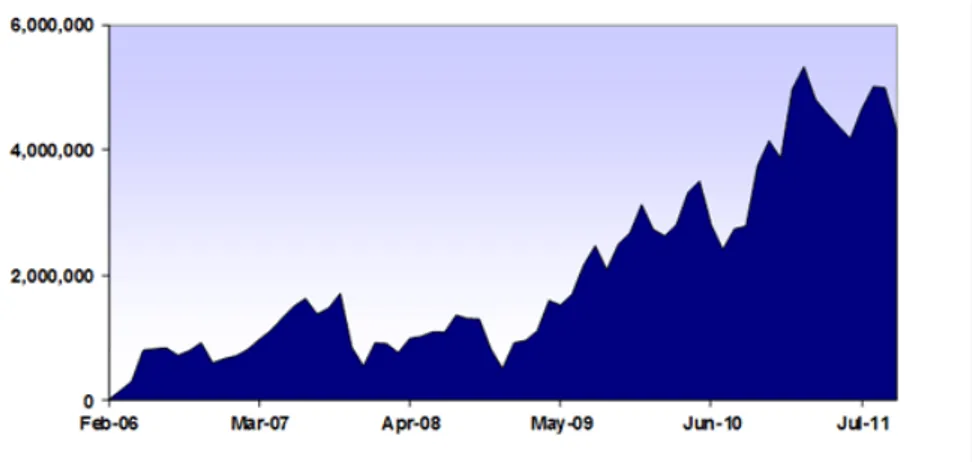
On March 24, 2004, CBOE introduced the first exchange-traded VIX futures contract on its new, all-electronic CBOE Futures Exchange. Two years later in February 2006, CBOE launched VIX options, the most successful new product in Exchange history: in less than five years, the com-bined trading activity in VIX options and futures has grown to more than 100,000 contracts per day.
3.1 The VIX calculation step-by-step
Stock indexes, such as the S&P 500, are calculated using the prices of their component stocks. Each index employs rules for selecting component options and a formula to calculate index values. VIX is a volatility index comprised of options rather than stocks, with the price of each option reflecting the market’s expectation of future volatility. Like conventional indexes, VIX employs rules that govern the selection of component options and a formula to compute index values.
1The Standard & Poor’s 100 Index is a capitalization-weighted index of 100 stocks from a broad range of indus-tries. The component stocks are weighted according to the total market value of their outstanding shares. The impact of a component’s price change is proportional to the issue’s total market value, which is the share price times the number of shares outstanding. These are summed for all 100 stocks and divided by a predetermined base value. The base value for the S&P 100 Index is adjusted to reflect changes in capitalization resulting from mergers, acquisitions, stock rights, substitutions, etc. Index options on the S&P 100 are traded with the ticker symbol “OEX”.
18 3. The CBOE Volatility Index - VIX
The generalized formula used in the VIX calculation is:
σ2 = ( 2 T X i ∆Ki Ki2 e r TQ(K i) − 1 T ·F K0− 1 ¸2) (3.1) where σ VIX 100, i.e. VIX = σ × 100 T Time to expiration
F Forward index level derived from index option prices
K0 First strike below the forward index level, F
Ki Strike price of the it hout-of-the-money option: − a call if Ki> K0
− a put if Ki< K0
− both put and call if Ki= K0.
∆Ki Interval between strike prices: ∆Ki=Ki +1− Ki −1 2
(Note. ∆K for the lowest strike is simply the difference between the lowest strike and the next higher strike. Likewise,∆K for the highest strike is the difference between the highest strike and the next lower strike.)
r Risk-free interest rate to expiration
Q(Ki) The midpoint of the bid-ask spread for each option with strike Ki.
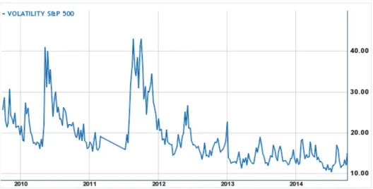
Figure3.1below depicts the VIX Index between September 2010 and September 2014. By read-ing the chart backwards we observe that by 2014 to early 2013 it tended to stay between 10 and 20; then it increased gradually until it spiked at over 40 in September and August 2011. By mid-2011 it had declined to more normal levels, but in April 2010 it reached a spike of 40. By March 2010 it finally declined to lower levels.
3.1 The VIX calculation step-by-step 19
Hereafter we provide all the necessary information about the way the VIX Index is calcu-lated.
The components of VIX are near- and next-term put and call options, usually in the first and second SPX contract months. “Near-term” options must have at least one week to expiration; a requirement intended to minimize pricing anomalies that might occur close to expiration. When the near-term options have less than a week to expiration, VIX “rolls” to the second and third SPX contract months. For the purpose of calculating time to expiration, SPX options are deemed to expire at the open of trading on SPX settlement day - the third Friday of the month. The VIX calculation measures time to expiration T in calendar days and divides each day into minutes, indeed it is given by the following expression:
T =©MCurrent day+ MSettlement day+ MOther days
ª Minutes in a year
where
MCurrent day Minutes remaining until midnight of the current day
MSettlement day Minutes from midnight until 8:30 a.m. on the SPX settlement day
MOther days Total minutes in the days between current day and settlement day. For example, if we assume that the near-term and the next-term options have 9 days and 37 days to expiration, respectively, using 8:30 a.m. as the time of the calculation T , the time for the near-term and next-term options, denoted by T1and T2, respectively, is calculated as follows
T1=930 + 510 + 11520
525600 = 0.0246575
T2=
930 + 510 + 51840
525600 = 0.1013699.
The risk-free interest rate r is the bond-equivalent yield of the U.S. T-bill maturing closest to the expiration dates of relevant SPX options. As such, the VIX calculation may use different risk-free interest rates for near- and next-term options. In this example, however, we assume that r = 0.38% for both sets of options.
Hereafter we present a representative sample of the VIX computation, the interim calculations will be a repetition of it.
STEP 1 - Select the options to be used in the VIX calculation.
The selected options are out-of-the-money SPX calls and out-of-the-money SPX puts centered around an at-the-money strike price, K0. Besides, only SPX options quoted with non-zero bid prices are used in the VIX calculation.
For each contract month:
• Determine the forward SPX level F by identifying the strike price at which the ab-solute difference between the call and put prices is smallest: the call and put prices reflect the average of each option’s bid/ask quotation.
20 3. The CBOE Volatility Index - VIX
In this example, the difference between the call and put prices is smallest at the 920 strike for both the near- and next-term options, thus using the put-call parity formula
F = Strike price + erτ(Call price − Put price)
the forward index prices, F1and F2 for the near- and next-term options, respec-tively, are
F1= 920 + e0.0038×0.0246575(37.15 − 36.65) = 920.50005
F2= 920 + e0.0038×0.1013699(61.55 − 60.55) = 921.00039.
• Determine K0, the strike immediately below the forward index level F for the near-and next-term options. In this example K0,1= K0,2= 920.
• Select out-of-the-money put options with strike smaller than K0. Start with the put strike immediately lower than K0and move to successively lower strike prices, ex-cluding any put options that have a bid price equal to zero. Finally, once two puts with consecutive strike prices are found to have zero bid prices, no puts with lower strikes are considered.
Then, select out-of-the-money call options with strike greater than K0. Start with the call strike immediately higher than K0 and move to successively higher strike prices, excluding any call options that have a bid price equal to zero. Equally to the puts, once two calls with consecutive strike prices are found to have zero bid prices, no calls with higher strikes are considered.
3.1 The VIX calculation step-by-step 21
Finally, select both the put and call with strike price K0. The K0put and call prices are averaged to produce a single value. In our example, the price used for the 920 strike in the near-term and in the next-term are, respectively,
(37.15 + 36.65)/2 = 36.90 (61.55 + 60.55)/2 = 61.05.
STEP 2 - Calculate volatility for both near-term and next-term options.
Applying the VIX formula (3.1) to the near-term and next-term options with time to expi-ration of T1and T2, respectively, yields:
σ12= 2 T1 X i ∆Ki Ki2 e r T1Q(K i) − 1 T1 ·F K0− 1 ¸2 σ22= 2 T2 X i ∆Ki Ki2 e r T2Q(Ki) − 1 T2 ·F K0− 1 ¸2
VIX is an amalgam of the information reflected in the prices of all of the selected options. The contribution of a single option to the VIX value is proportional to∆K and the price of that option, and inversely proportional to the square of the option’s strike price.
22 3. The CBOE Volatility Index - VIX
In our example the contribution of the near-term 400 Put is given by: ∆K400 Put K400 Put2 e r T1Q(400Put) = 25 4002e 0.0038×0.0246575 × 0.125 = 0.0000195
and a similar calculation is performed for each option. The resulting values for the near-term options are then summed and multiplied by T12. Likewise, the resulting values for the next-term options are summed and multiplied by T22. The table below summarizes the results for each strip of options.
Next, we calculateT1hK0F − 1i2for the near-term T1and the next-term T2. 1 T1 ·F 1 K0− 1 ¸2 = 1 0.0246575 · 920.50005 920 − 1 ¸2 = 0.0000120 1 T2 ·F 2 K0− 1 ¸2 = 1 0.1013699 · 921.00039 920 − 1 ¸2 = 0.0000117. Finally, we computeσ21andσ22:
σ12= 2 T1 X i ∆Ki Ki2 e r T1Q(K i) − 1 T1 · F K0− 1 ¸2 = 0.4727799 − 0.0000120 = 0.4727679 σ22= 2 T2 X i ∆Ki Ki2 e r T2Q(K i) − 1 T2 · F K0− 1 ¸2 = 0.3668297 − 0.0000117 = 0.3668180.
STEP 3 - Calculate the 30-day weighted average ofσ21andσ22, take the square root of that value and multiply by 100 to get the VIX.
VIX = 100 × s ½ T1σ21 ·N T2− N30 NT2− NT1 ¸ + T2σ22 ·N 30− NT1 NT2− NT1 ¸ ×N365 N30 ¾ .
3.1 The VIX calculation step-by-step 23
When the near-term options have less than 30 days to expiration and the next-term op-tions have more than 30 days to expiration, the resulting VIX value reflects an interpola-tion ofσ21andσ22; i.e., each individual weight is less than or equal to 1 and the sum of the weights equals 1. At the time of the VIX “roll”, instead, both the near-term and next-term options have more than 30 days to expiration: the same formula is used to calculate the 30-day weighted average, but the result is an extrapolation ofσ21andσ22; i.e., the sum of the weights is still 1, but the near-term weight is greater than 1 and the next-term weight is negative.
Returning to our example we finally get
NT1 Number of minutes to settlement of the near-term options (12, 960)
NT2 Number of minutes to settlement of the next-term options (53, 280)
N30 Number of minutes in 30 days (30 × 1,440 = 43,200)
N365 Number of minutes in a 365-day year (365 × 1,440 = 525,600) and VIX = 100 × s ½ 0.0246575 × 0.4727679 ×· 53, 280 − 43,200 53, 280 − 12,960 ¸ + 0.1013699 × 0.3668180 × s · 43, 200 − 12,960 53, 280 − 12,960 ¸ ×525, 600 43, 200 ) whence VIX = 100 × 0.612179986 = 61.22.
24 3. The CBOE Volatility Index - VIX
3.2 VIX Squared and Forward Price of Integrated Variance
In this section we derive the probabilistic representation of the square of the VIX, indeed we will prove that it can be interpreted as the conditional risk-neutral expectation of a log con-tract. Before proceeding, we state beforehand the definition of the VIX squared we are go-ing to use hereafter. Since the purpose of this work is to price European options on the VIX under continuous-time jump-diffusion models, we should be able to provide the correspond-ing continuous-time version for the definition of VIX squared (3.1). As a matter of fact, it is straightforward to extend the previous discrete definition (3.1) to the continuous case, simply by assuming to take the limit as∆K −→ 0. Indeed we have
VIX2= 1002×½ 2 τ ·Z F 0 1 y2P (y) d y +˜ Z ∞ F 1 y2C (y) d y˜ ¸¾ (3.2)
where ˜P (y) and ˜C (y) represent forward put and call prices with strike y, respectively. We
no-tice that the termhK0F − 1i2has disappeared from the new expression for the square of the VIX, since K0, being the first strike immediately below the forward index level F , tends to equalize the value F as∆K tends to zero.
THEOREM - 3.2.1. The risk-neutral probability density function of the stock price S at time T is
given by f (ST, T ; St, t ) =∂ 2C (S˜ t, x, t , T ) ∂x2 ¯ ¯ ¯ x=ST (3.3) or, equivalently, f (ST, T ; St, t ) =∂ 2P (S˜ t, x; t , T ) ∂x2 ¯ ¯ ¯ x=ST (3.4)
where ˜C and ˜P represent forward call and put prices, respectively:
˜
C (St, x; t , T ) = er (T −t)C (St, x; t , T ) ˜
P (St, x; t , T ) = er (T −t)P (St, x; t , T ).
Proof. For the sake of simplicity, in the following, we denote the risk-neutral probability density
function of ST, conditional onFt, as follows
f (·) := f (·,T ;St, t ). For every measurable functionφ, we have
Z ∞ 0 φ(x) ∂2C (S˜ t, x; t , T ) ∂x2 d x = Z ∞ 0 φ(x)e r (T −t)∂2C (St, x; t , T ) ∂x2 d x = Z ∞ 0 φ(x)e r (T −t) ∂2 ∂x2e −r (T −t )EQ£(ST − x)+|St¤ d x = Z ∞ 0 φ(x) ∂2 ∂x2 Z Ω(ST− x) +dQ d x = Z ∞ 0 φ(x) ∂2 ∂x2 Z ∞ 0 (y − x) +f (y) d y d x
3.2 VIX Squared and Forward Price of Integrated Variance 25 = Z ∞ 0 φ(x) ∂2 ∂x2 Z ∞ x (y − x) f (y) d y d x = Z ∞ 0 φ(x) ∂ ∂x µ ∂ ∂x Z ∞ x y f (y) d y − ∂ ∂x Z ∞ x x f (y) d y ¶ d x = Z ∞ 0 φ(x) ∂ ∂x µ − ∂ ∂x Z x ∞y f (y) d y + ∂ ∂xx Z x ∞ f (y) d y ¶ d x
(by the fundamental theorem of calculus) = Z ∞ 0 φ(x) ∂ ∂x µ −x f (x) + Z x ∞f (y) d y + x f (x) ¶ d x = Z ∞ 0 φ(x) ∂ ∂x µZ x ∞ f (y) d y ¶ d x = Z ∞ 0 φ(x)f (x) dx. Hence ∂2C (S˜ t, x; t , T ) ∂x2 ¯ ¯ ¯ x=ST
is the probability density function of ST. Analogously, in the case of put options, we have, for every measurable functionφ
Z ∞ 0 φ(x) ∂2P (S˜ t, x; t , T ) ∂x2 d x = Z ∞ 0 φ(x)e r (T −t)∂2P (St, x; t , T ) ∂x2 d x = Z ∞ 0 φ(x)e r (T −t) ∂2 ∂x2e −r (T −t )EQ£(x − ST )+|St¤ d x = Z ∞ 0 φ(x) ∂2 ∂x2 Z Ω(x − ST) +dQ d x = Z ∞ 0 φ(x) ∂2 ∂x2 Z Ω(x − y) +PST(d y) d x = Z ∞ 0 φ(x) ∂2 ∂x2 Z ∞ 0 (x − y) +f (y) d y d x = Z ∞ 0 φ(x) ∂2 ∂x2 Z x 0 (x − y)f (y) d y d x = Z ∞ 0 φ(x) ∂ ∂x µ ∂ ∂x Z x 0 x f (y) d y − ∂ ∂x Z x 0 y f (y) ¶ d x
(by the fundamental theorem of calculus) = Z ∞ 0 φ(x) ∂ ∂x µ ∂ ∂x µ x Z x 0 f (y) d y ¶ − x f (x) ¶ d x = Z ∞ 0 φ(x) ∂ ∂x µZ x 0 f (y) d y + x f (x) − x f (x) ¶ d x = Z ∞ 0 φ(x)f (x) dx. Thus ∂2P (S˜ t, x; t , T ) ∂x2 ¯ ¯ ¯ x=ST