Alma Mater Studiorum · Universit`
a di Bologna
FACOLT `A DI SCIENZE MATEMATICHE, FISICHE E NATURALI
Corso di Laurea Specialistica in Informatica
Structure Learning of Graphical Models
for
Task-Oriented Robot Grasping
Relatore:
Chiar.mo Prof.
Sandro Rambaldi
Correlatori:
Chiar.ma Prof.ssa
Danica Kragic
Dr.ssa Dan Song
Dr. Kai Huebner
Presentata da:
Alessandro Pieropan
II Sessione
Contents
1 Introduction 1
2 Bayesian Networks 5
2.1 Overview . . . 5
2.2 Structure Learning Background . . . 7
2.2.1 Discretization . . . 8
2.2.2 Structure Learning Methods . . . 10
2.3 Parameter Learning Background . . . 12
2.4 Our approach . . . 12
2.5 Structure Learning Algorithms . . . 13
2.6 Summary of Bayesian Network . . . 14
3 Structure Learning Experiments on Well-Known Networks 15 3.1 Overview . . . 15
3.2 Discretization experiment on Incinerator network . . . 17
3.2.1 Car and Insurance network experiments . . . 20
3.3 Consideration After the Experiments . . . 22
3.3.1 Edge Average Matrix Approach . . . 23
3.3.2 Network Decomposition approach . . . 23
3.3.3 BIC Score Search Approach . . . 26
3.4 Summary of Experiments . . . 27
4 Grasp Planning 29 4.1 Overview . . . 29
4.2 Experiments on grasp planner data . . . 31
4.2.1 Real data overview . . . 31
4.2.2 Dimensionality Reduction . . . 33
4.2.3 Discretization . . . 33
4.2.4 Structure learning . . . 33
4.2.5 Parameter Learning and Testing . . . 35
4.3 Grasp Planners Comparison . . . 36
4.4 Summary of Real Data Analysis . . . 37
5 Discussion 39 5.1 Limitation . . . 39
5.2 Future Work . . . 39
5.2.1 Discretization Future Work . . . 39
5.2.2 Structure Learning Future Work . . . 40
5.2.3 Grasp Planner Integration . . . 41
A Code Overview 43 A.1 Multivariate Discretization Class . . . 43
A.2 Node Discretization . . . 47
A.3 Structure Learning . . . 47
A.4 Example . . . 49
List of Figures
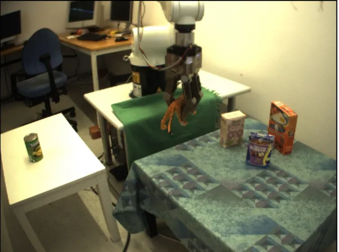
1.1 Grasping example. . . 1
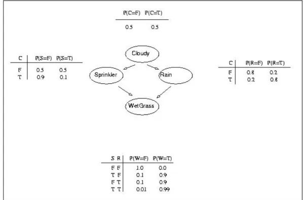
2.1 Example of a Bayesian network for the wet grass problem. . . 6
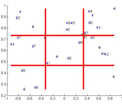
2.2 Example of discretization from bi-dimensional data, the numbered points are continuous data and the areas defined by the edges are the discrete values. In this case we want to discretize the data into 9 possible discrete states. . . 8
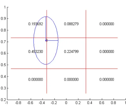
2.3 Example of soft discretization in 2 dimensions and how the discrete states are affected by the spreading function. . . 9
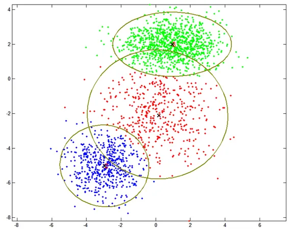
2.4 Overview of Gaussian mixture model (GMM) approach to discretize data. In the example it can be seen the distribution of sample bi-dimensional data and the components calculated by the algorithm. . . 10
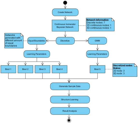
3.1 Activity diagram showing the experiment made with Incinerator network. First, we discretize the mixed network with two different approaches: Gaussian Mixture Model (Bnet 5) and Equal Boundaries. Four differ-ent networks are discretized with Equal boundaries approach changing the number of discrete boundaries (Eqb 1,2,3,4). . . 16
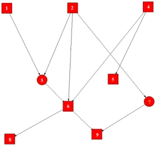
3.2 Structure of the modified Incinerator network with 7 discrete nodes and 2 continuous nodes. . . 17
3.4 Original structure of Car network . . . 21
3.3 Original structure of Insurance network . . . 21
3.5 Original Car Dag with edge matrix results. . . 25
3.6 BIC tree search approach overview. Here the tree is expanded to level 2 as example. . . 26
4.1 Complete system diagram. The selected grasp planner generates a grasp given a robotic hand and an object as an input. The generated grasp is then calculated by the simulation environment GraspIt and all the features are extracted from it and the human expert label the grasp looking at the visualization. The features are then stored to be used to train and testing the Bayesian network framework. . . 30 4.2 Activity diagram for the complete experiment procedure on data of the
selected grasp planner. . . 32 4.3 Activity diagram for real data structure learning . . . 34 4.4 Resulting Bayesian network after structure learning and inference tests. . 36
A.1 Multivariate Discretization Class Diagram . . . 44 A.2 Mutivariate Discretization Activity Diagram . . . 48
List of Tables
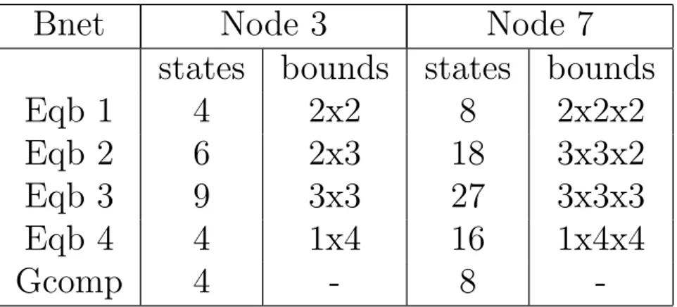
3.1 Number of discrete states for the Bayesian networks nodes created after discretization. Eqb 1 to 4 are discrete networks where the continuous nodes of the ground truth network are discretized with the equal boundary approach while Gcomp is discretized using Gaussian Mixture Models. . . 18 3.2 Percentage of runs that return a network’s structure exactly the same as
the ground truth. . . 18 3.3 Summary of the results given by the algorithms used for structure learning
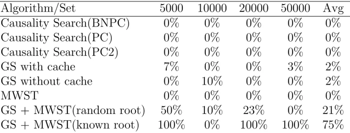
of the network Eqb3. Results are for three different algorithm with vari-ous settings: Causality Search (PC), Greedy Search (GS) and Maximum Weight Spanning Tree (MWST). Results are in percentage of runs that return a network equal to the ground truth. . . 19 3.4 Summary of the results given by the algorithms used for structure learning
of the network Gcomp. Results are in percentage of runs that return a network equal to the ground truth. . . 19 3.5 Percentage of runs for Eqb3 that return a structure with differences in
edges from the ground truth between 1 and 5. . . 20 3.6 Percentage of runs for Gcomp that return a structure with differences in
edges from the ground truth between 1 and 5. . . 20 3.7 Car network learning resulting matrix with ‘divide and conquer’ approach
and 6000 data. Survey percentages for original network edges are in bold. It can be seen that only edge from node 7 to 8 is not found at all and edge from node 8 to 11 has a low percentage but the precision increase with a higher number of data. . . 24
3.8 Car network reconstruction with 15000 data points considering an edge when the probability in the edge matrix is higher than 75. It can be seen
that the calculated DAG is equal to the ground truth. . . 25
4.1 Task and Actions structure learning. . . 34
4.2 Task and Objects structure learning. . . 35
4.3 Task and Constraints structure learning. . . 35
4.4 Confusion matrix for the task inference test. T1 is hand-over, T2 pouring and T3 tool-use. . . 36
Chapter 1
Introduction
Figure 1.1: Grasping example.
In the collective imaginaries a robot is a human like machine as any androids in science fiction. However the type of robots that you will encounter most frequently are machinery that do work that is too dangerous, boring or onerous. Most of the robots in the world are of this type. They can be found in auto, medical, manufacturing and space industries. Therefore a robot is a system that contains sensors, control systems, manipulators, power supplies and software all working together to perform a task. The development and use of such a system is an active area of research and one of the main problems is the development of interaction skills with the surrounding environ-ment, which include the ability to grasp objects. To perform this task the robot needs to sense the environment and acquire the object informations, physical attributes that may influence a grasp. Humans can solve this grasping problem easily due to their past experiences, that is why many researchers are approaching it from a machine learning perspective finding grasp of an object using information of already known objects. But humans can select the best grasp amongst a vast repertoire not only considering the physical attributes of the object to grasp but even to obtain a certain effect. This is why in our case the study in the area of robot manipulation is focused on grasping and inte-grating symbolic tasks with data gained through sensors. The learning model is based on Bayesian Network to encode the statistical dependencies between the data collected by the sensors and the symbolic task. This data representation has several advantages. It allows to take into account the uncertainty of the real world, allowing to deal with sensor noise, encodes notion of causality and provides an unified network for learning. Since the network is actually implemented and based on the human expert knowledge, it is very interesting to implement an automated method to learn the structure as in the future more tasks and object features can be introduced and a complex network design based only on human expert knowledge can become unreliable. Since structure learning algorithms presents some weaknesses, the goal of this thesis is to analyze real data used in the network modeled by the human expert, implement a feasible structure learning approach and compare the results with the network designed by the expert in order to possibly enhance it. The rest of the thesis is organized as follows. Chapter II will present Bayesian network and explain the weaknesses that justify our approach. Chapter III will introduce our approach to structure learning. Chapter IV will outline the experimental
3
results, and Chapter V will present conclusions.
Nell’immaginario collettivo un robot solitamente `e una macchina umanoide come gli androidi nella fatascienza. Tuttavia i robot che si possono incontrare pi`u spesso sono macchinari che svolgono lavori troppo pericolosi, noiosi, ripetitivi o semplicemente dif-ficili. La maggior parte dei robot sono di questo tipo. Vengono spesso usati nel settore automobilistico, medico, manifatturiero e spaziale.
Un robot `e quindi un sistema composto da sensori, sistemi di controllo, manipolatori, fonti energetiche e un software, tutte parti che insieme svolgono un compito. Lo sviluppo e l’uso di un tal sistema `e un campo attivo della ricerca e uno dei problemi maggiori consiste nello sviluppo di capacit`a di interazione con l’ambiente circostante, inclusa la capacit`a di afferrare oggetti. Per portare a termine questo compito il robot ha bisogno di percepire l’ambiente esterno e acquisire le informazioni relative all’oggetto, gli attributi fisici che potrebbero influenzare la presa. Gli esseri umani possono portare a termine questo compito molto facilmente grazie alla loro esperienza, ed `e proprio per questo che i ricercatori affrontano questo problema nel campo dell’apprendimento automatico, em-ulando il comportamento umano e cercando una possibile presa usando le informazioni ottenute da oggetti gi`a conosciuti. Tuttavia gli essere umani non solo scelgono una possi-bile presa considerando gli attributi fisici dell’oggetto ma tengono anche in considerazione il fine di tale azione. Ecco perch`e nel nostro caso, la ricerca nel campo dell’interazione robotica si focalizza nell’integrare dati fisici ottenuti dai sensori con informazioni sim-boliche rappresentanti il fine dell’azione. Il nostro modello di apprendimento `e basato sulle Reti Bayesiane per integrare le dipendenze statistiche tra i dati raccolti dai sensori e gli obiettivi simbolici. Questo tipo di rappresentazione ha diversi vantaggi. Permette di tener in considerazione l’incertezza del mondo reale, gestendo il disturbo nelle rilevazioni dei sensori, incapsulare nozioni di causalit`a a fornire un rete unica per l’apprendimento. Dato che l’implementazione della rete utilizzata `e basata unicamente sulle conoscienze di un esperto, siamo interessati a implementare un sistema automatico per apprendere la struttura dei dati siccome in futuro potranno venir aggiunti pi`u obiettivi e oggetti aumentando cos`ı la complessit`a della rete e rendendo la progettazione manuale basata solo sul giudizio umano inaffidabile. Gli obiettivi di questa tesi sono di analizzare i
dati usati dalla rete progettata manualmente, implementare un possibile approccio per l’apprendimento che possa ovviare alle debolezze degli algoritmi di apprendimento e confrontare i risultati ottenuti con la rete progettata dall’esperto umano possibilmente incrementandone le prestazioni. La tesi `e organizzata come segue. Il Capitolo II presenta le reti Bayesiane e evidenzia le debolezze che giustificano il nostro approccio. Il Capi-tolo III descrive il nostro approccio per l’apprendimento della struttura. Il CapiCapi-tolo IV illustra i nostri risultati mentre nel Capitolo V vengono presentate le nostre conclusioni e sviluppi futuri.
Chapter 2
Bayesian Networks
2.1
Overview
Bayesian network (BN), also known as belief networks belong to the family of prob-abilistic graphical models. These graphical structures are used to represent knowledge about an uncertain domain. In particular, each node in the graph represents a random variable, while the edges between the nodes represent probabilistic dependencies among the corresponding random variables. Our specific problem is to use Bayesian networks in robotics to encode the statistical dependencies between objects attributes, grasp actions and a set of task constraints, and use the model as a knowledge base that allows robots to reason at a high-level manipulation tasks. Since the input data is usually continu-ous and noisy, the problem is very high-dimensional and has complex distribution on many variables, that is why we choose to use Bayesian network as it provides a good representation of the joint distribution of such complex problem domains. A Bayesian network is a probabilistic graphical model that represent a set of random variables and their dependencies using a directed acyclic graph (DAG) where every node is labeled with a specific probabilistic information [18],[19],[25],[17]. The full specification [28] is the following.
1. A set of random variables makes up the nodes of the network. Variables may be discrete or continuous.
2. A set of directed links or edges connects pair of nodes. If there is an edge from node X to node Y, X is said to be a parent of Y.
3. Each node Xi has a conditional probability distribution P (Xi|Parents (Xi)) that
quantifies the effect of the parents on the node.
4. The graph has no directed cycles (and hence, is a directed, acyclic graph or DAG).
Figure 2.1: Example of a Bayesian network for the wet grass problem.
The topology of the network, as it can be seen in the example in Fig. 2.1, specifies the conditional independence relationships that hold in the domain. Any arrow from a node X to a node Y (e.g X = Cloudy, Y = rain) implies that X has a direct influence on Y. Once the topology of the network is defined, it is needed to specify the proba-bility distribution of each variable, given its parents. In the figure each distribution is represented as a conditional probability table (CPT). Each row in the CPT show the conditional probability of the variable for a conditioning case. A conditioning case is simply a combination of the parents value. A network provides a complete description
2.2 Structure Learning Background 7
of the domain. Every entry in the full joint probability distribution can be calculated from network. Every entry value, denoted by P (X1 = x1 ∧ ... ∧ Xn = xn), is given by
the formula:
P (X1 = x1∧ ... ∧ Xn = xn) =
Qn
i=1P (Xi|Parents (Xi)).
2.2
Structure Learning Background
Usually the network is specified by an expert and then it is used to perform infer-ence. But in complex cases it is not feasible and unreliable. In these cases the network structure is learned from data using an automated method. There are two very different approaches to structure learning: based and search-and-score. The constraint-based approach starts with a fully connected graph and remove edges when a certain condition is met. The search-and-score approach performs a search through the space of possible DAGs, and returns the best one found using a scoring function. Using an automated method to learn the Bayesian network structure of a system or environment gives researchers useful information about the causal relationships among variables. But it is very hard to learn the network when we have to handle continuous data especially when distribution is not Gaussian or when we have to deal with a case that is not full ob-served having missing data or hidden variables. As a consequence most Bayesian network structure learning algorithms work with discrete data. As data are often continuous and networks really complex, a common approach to learn the structure with an automated method is to previously discretize the data.
2.2.1
Discretization
Figure 2.2: Example of discretization from bi-dimensional data, the numbered points are continuous data and the areas defined by the edges are the discrete values. In this case we want to discretize the data into 9 possible discrete states.
In statistics and machine learning, discretization refers to the process of converting continuous features or variables to discretized or nominal features. There are two possible approach of discretization:
Hard : consists of defining boundaries for the data we want to discretize and turning the continuous features into discrete ones usually using a proximity function. As in Fig. 2.2 an area delimited by red edges is a discrete value and every continuous data point inside it assume the discrete value of that area. Looking at the example, the continuous data point number 23 will be turned to the discrete value of 1, assuming we number the discrete areas from top left corner to bottom right.
Soft : the continuous value is not turned directly to the value of the nearest bound but its value is ‘spread’ to other possible discrete values using a spreading function. This
2.2 Structure Learning Background 9
method, suggested by Imme Ebert-Uphoff [7], has a linear Gaussian distribution as spreading function and the deviation value of the distribution determines how much every continuous data point will be spread over the discrete boundaries. With a deviation equal to zero the soft discretization behave exactly as the hard one.
Soft Discretization with Multidimensional Spreading Function
Following this idea we implemented an algorithm that, given high-dimensional data and a list of bounds, soft discretizes them using a multidimensional gaussian distribution and learns the parameters of the built discrete Bayesian network using the soft evidences as in Fig. 2.3.
Figure 2.3: Example of soft discretization in 2 dimensions and how the discrete states are affected by the spreading function.
Gaussian Mixture Models
Figure 2.4: Overview of Gaussian mixture model (GMM) approach to discretize data. In the example it can be seen the distribution of sample bi-dimensional data and the components calculated by the algorithm.
Gaussian Mixture Models (GMMs) are among the most statistically mature methods for clustering. It consists in the assignment of a set of observations into subsets (called clusters) so that observations in the same cluster are similar in some sense. Clusters are assigned by selecting the component that maximizes the posterior probability.
2.2.2
Structure Learning Methods
There are three different approaches for structure learning for continuous data re-gardless of the specific algorithm used for the structure learning [11]:
al-2.2 Structure Learning Background 11
gorithm. There are different techniques for the discretization of data. The most common one could be Equal-width and Equal-frequency binning. In the first case the range of values for each variable is divided into k equally sized intervals where k is pre-defined. Arbitrary values of k are usually chosen but there are also other methods [20] to determine values of k. Equal-frequency binning, on the other hand, assigns to each interval an equal number of values.
Integrated Discretization : The integrated approaches [9],[22],[31] require a starting discretization, usually equal-frequency binning, and they hold the discretization fixed while learning the structure and hold the learning while discretizing. The procedures stop repeating when the termination condition is met.
Direct : These approaches adapt the learning of the structure to handle continuous data [1],[30].
All the approaches are evaluated and compared in terms of quality of the structure learned and efficiency of the process [11]. The data used for the comparison are both gen-erated from well-known Bayesian networks and from real data with unknown structure. The simulated data produced for the comparison use some well-known networks(e.g. Alarm) with a number of variables between 20 and 56 and edges between 25 and 66. For pre and integrated discretization approaches the number of possible discrete values k is 2 or 3 and for each network different sets of data are generated with size from 500 to 5000. It seems that the best overall method is the direct, as it works well both for simulated and real data but still all the approaches have good and bad points to take into consideration.
1. The number of discrete values k for pre and integrated discretization methods is really small and independent from the distribution of continuous data, as we notice in our test on Incinerator network (Sec. 3.2) as we increase the number of discrete values the accuracy increase but with a cost in complexity.
2. The discretization used by Lawrence Fu in his work [11] is only hard and it could be interesting to see how a soft discretization approach could influence the learning of the structure of a network.
3. A discretized approach could include other possible benefits like the efficiency of the learning algorithms and the aid in understanding the data [6], and if it is believed that variables are naturally discrete but there are continuous due to noise, then discretization is justified [12]. On the other hand even with soft discretization there is still a loss of information.
4. The learning is very hard when we have to deal with missing data or hidden nodes in the network.
5. Direct methods threats all data as Gaussian and this can not be good when we have to deal with continuous data with a different distribution.
Considering all the weaknesses of learning approaches and the nature of real data we want to analyze, we think that a feasible learning approach can be one base on the pre-discretization of data.
2.3
Parameter Learning Background
Assuming we have already defined or learned the structure of the network, to fully represent the joint probability distribution, it is necessary to specify for each node X the probability distribution. The data we use for the structure learning can be con-sidered evidences, instantiation of some or all of the random variables describing the domain. Given evidences the learning process basically calculates the probability of each hypothesis and makes prediction of that basis.
2.4
Our approach
The Bayesian network we want to analyze is developed in Matlab using the BNT package [24] and it is built using both continuous and discrete nodes, in particular continuous node are determined by multidimensional data. For this reason the first thing to do is to study a possible discretization approach to turn the continuous nodes into discrete nodes. Studying the BNT soft discretization package we use a soft discretization approach for our data using a spreading function following the idea given by Imme
2.5 Structure Learning Algorithms 13
Ebert-Uphoff [7]. However the soft discretization package gives an algorithm for linear continuous data so we enhance this approach to use a spreading function into more dimensions. The soft discretized data could be later used for parameter learning.
2.5
Structure Learning Algorithms
Usually a Bayesian network is specified by an expert and is then used to perform inference. However, defining the network structure by human expert is not easy, es-pecially when many variables are included. For this reason automatically learning the structure of a Bayesian network is a problem pursued within machine learning. The basic is to develop an algorithm to recover the structure of the direct acyclic graph (DAG) of the network. The first and simple idea could be to evaluate all the possible graph of a network and choose the best one. Since this solution has a high complexity it is only feasible to make an exhaustive search with decent performances for networks with at least 8 nodes [27]. Given that the majority of algorithms used in structure learning use search heuristics. In the following sections we introduce some of the algorithms of the BNT structure learning package [8] used for learning in our tests.
Causality Search : the PC algorithm (after its authors, Peter and Clark) [30], [26] use a statistical test to evaluate the conditional dependencies between variables and the result is evaluated to build the network structure.
Maximum Weight Spanning Tree : (MWST) [3] given a graph G, calculates a span-ning tree (subgraph of G) that contains all the vertices of G. The algorithm asso-ciates a weight to each edge that could be either the mutual information between the two variables [3] or the score variation when a node becomes a parent of an-other [14]. The algorithm needs an initialization node considered the root of the tree.
K2 : algorithm heuristically searches for the most probable network structure given the data. The algorithm requires an order over the nodes of the network that could be an uniform prior of the structure or a topological order over the nodes where a
node can only be parent of a lower-ordered node. According to the given order as input the first node can’t have any parent [4].
Greedy Search : (GS) is an algorithm that follows the heuristic of choosing the local optimal at each stage with the hope of finding the global optimum. In network structure learning the algorithm takes an initial graph, calculate the neighborhood, compute the score for every DAG in the neighborhood and choose the best one as starting point for the next iteration. A neighbor of the DAG G is a defined as a graph that differ from G by one insertion, reversion or deletion of an edge.
2.6
Summary of Bayesian Network
In this chapter we introduced Bayesian networks, a probabilistic graphical model that we use as a knowledge base that allows robots to reason at a high-level manipulation tasks. We decide to use this model because the input of our problem is continuous, noisy and very high-dimensional and Bayesian network provides a good representation of the joint distribution of such complex problem domains. We want to implement an approach to learn the structure automatically because it is not feasible and unreliable for an expert to specify a network in complex cases. We introduced the most common approaches to learn the structure of a network underlining the weaknesses to understand which one can be used in our case. We also introduced the most frequently used learning algorithms that we use in our experiments to develop our approach to learn the structure of our network.
Chapter 3
Structure Learning Experiments on
Well-Known Networks
3.1
Overview
Before learning the structure of real data generated by the selected grasp planner we decided to study the behavior of both discretization and structure learning using well-known Bayesian networks as ground truth networks. Using sampled data from different networks we want to test how each algorithm performs in term of recover the true structure of the network and the quality of it using a Bayesian scoring function. Our tests focus on the following matters to discover any possible problem.
Discretization : in our tests we use equal-binning and GMMs approach. We desire to know how they can influence the learning, which one is working better and how the learning differ if we change the number of boundaries or components of the discretization.
Learning algorithm : we use different algorithms in our tests to compare the perfor-mances and discover the weaknesses.
Complexity : we want to figure out how the learning behaves if we increase the number of nodes of the network we want to learn.
Size of dataset : we want to figure out the algorithms performances with different datasets. The aim is to detect algorithms that perform well with a datasets of a size as small as the real data produced by the selected grasp planner.
The Bayesian networks we used for our purposes are Incinerator [5], Car [13] and In-surance [10] respectively composed by 9, 12 and 27 nodes. Our experiments highlight that increasing the number of components or boundaries of the discretization the learn-ing have a significant improvement but that costs in efficiency. Moreover learnlearn-ing the structure of networks with a high number of nodes is really hard. Given those problems, we develop new approaches illustrated later to address them.
Figure 3.1: Activity diagram showing the experiment made with Incinerator network. First, we discretize the mixed network with two different approaches: Gaussian Mixture Model (Bnet 5) and Equal Boundaries. Four different networks are discretized with Equal boundaries approach changing the number of discrete boundaries (Eqb 1,2,3,4).
3.2 Discretization experiment on Incinerator network 17
3.2
Discretization experiment on Incinerator network
Figure 3.2: Structure of the modified Incinerator network with 7 discrete nodes and 2 continuous nodes.
The first test used the well known Incinerator Bayesian network of 9 nodes but with some changes because we wanted to test structure learning with a discretized network. The network used in the experiment has the same DAG (Fig.3.2) as the original one but the nodes are modified as follows:
• Discrete nodes: 1,2,4,5,6,8,9
• 2-dimensional gaussian mixture node: 3 • 3-dimensional gaussian mixture node: 7
The data for node 3 and 7 were generated by some multiple dimensional Gaussian distributions. Given that Bayesian network with both continuous and discrete nodes, the aim of the test was to figure how the learning of the structure could be influenced by the discretization of the data for the continuous nodes. For that reason first of all we discretized the continuous node data with two different approaches: the Gaussian mixture approach to find clusters as it can be seen in Fig.2.4 and equal space subdivision
where data are spread in areas of the same width as in the example in Fig.2.2. Using this approach we built different Bayesian networks with discretized data for the continuous nodes as in Fig. 3.1.
Bnet
Node 3
Node 7
states
bounds
states
bounds
Eqb 1
4
2x2
8
2x2x2
Eqb 2
6
2x3
18
3x3x2
Eqb 3
9
3x3
27
3x3x3
Eqb 4
4
1x4
16
1x4x4
Gcomp
4
-
8
-Table 3.1: Number of discrete states for the Bayesian networks nodes created after discretization. Eqb 1 to 4 are discrete networks where the continuous nodes of the ground truth network are discretized with the equal boundary approach while Gcomp is discretized using Gaussian Mixture Models.
Bnet
5000
10000
20000
50000
Avg
Eqb 1
0%
0%
0%
8%
1%
Eqb 2
0%
9%
0%
10%
5%
Eqb 3
0%
19%
2%
28%
13%
Eqb 4
0%
1%
4%
13%
4%
Gcomp
0%
12%
12%
2%
7%
Table 3.2: Percentage of runs that return a network’s structure exactly the same as the ground truth.
The Table 3.2 shows the percentage of times that a learning algorithm returned the ground truth network structure. It could be seen that for a dataset of 5000 we never have the original network back but increasing the number of data the methods become much more accurate. It can be also noticed that the network discretized with equal boundaries (Eqb 3) and the one discretized with the Gaussian Mixture Model (Gcomp) can recover
3.2 Discretization experiment on Incinerator network 19
the ground truth network more often for two different reasons. The network Eqb 3 is the equal boundary network with most states for continuous nodes granting a refined discretization. On the other hand Gcomp has less states but as the continuous data are generated by multiple Gaussian distributions, this approach works perfectly with them. After this first run we decided to proceed with further analysis on Eqb 3 and Gcomp to find the algorithms that work the best.
Algorithm/Set
5000
10000
20000
50000
Avg
Causality Search(BNPC)
0%
0%
0%
0%
0%
Causality Search(PC)
0%
0%
0%
0%
0%
Causality Search(PC2)
0%
0%
0%
0%
0%
GS with cache
7%
0%
0%
3%
2%
GS without cache
0%
10%
0%
0%
2%
MWST
0%
0%
0%
0%
0%
GS + MWST(random root)
50%
10%
23%
0%
21%
GS + MWST(known root)
100%
0%
100%
100%
75%
Table 3.3: Summary of the results given by the algorithms used for structure learning of the network Eqb3. Results are for three different algorithm with various settings: Causal-ity Search (PC), Greedy Search (GS) and Maximum Weight Spanning Tree (MWST). Results are in percentage of runs that return a network equal to the ground truth.
Algorithm/Set
5000
10000
20000
50000
Avg
Causality Search(BNPC)
0%
0%
0%
0%
0%
Causality Search(PC)
0%
0%
0%
0%
0%
Causality Search(PC2)
0%
0%
0%
0%
0%
GS with cache
0%
0%
0%
0%
0%
GS without cache
0%
0%
0%
0%
0%
MWST
0%
0%
0%
0%
0%
GS + MWST(random root)
0%
0%
13%
0%
3%
GS + MWST(known root)
100%
100%
0%
0%
50%
Table 3.4: Summary of the results given by the algorithms used for structure learning of the network Gcomp. Results are in percentage of runs that return a network equal to the ground truth.
Algorithm/Set
5000
10000
20000
50000
Avg
Causality Search(BNPC)
0%
0%
0%
100%
0%
Causality Search(PC)
0%
0%
0%
0%
0%
Causality Search(PC2)
0%
0%
0%
0%
0%
GS with cache
7%
17%
10%
17%
2%
GS without cache
20%
10%
3%
27%
2%
MWST
0%
0%
0%
0%
0%
GS + MWST(random root)
20%
63%
37%
50%
21%
GS + MWST(known root)
0%
100%
0%
0%
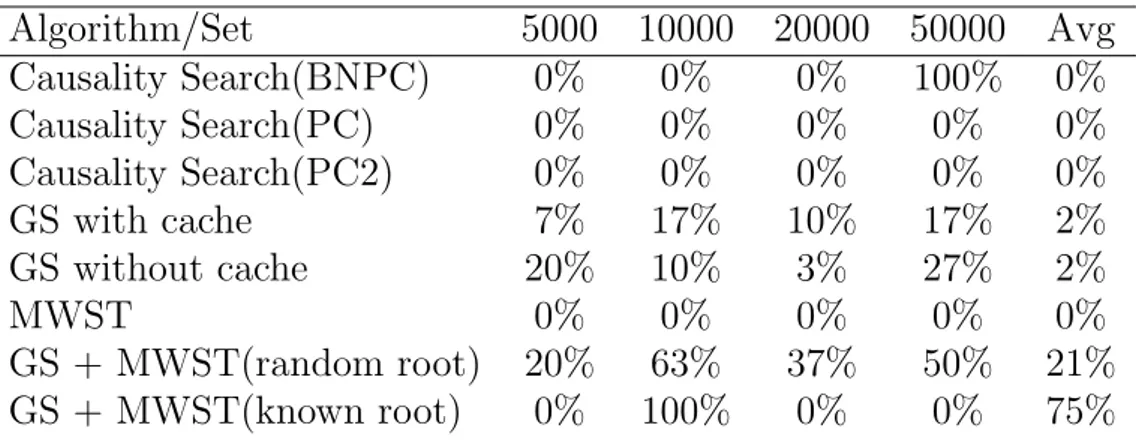
75%
Table 3.5: Percentage of runs for Eqb3 that return a structure with differences in edges from the ground truth between 1 and 5.
Algorithm/Set
5000
10000
20000
50000
Avg
Causality Search(BNPC)
0%
100%
100%
100%
75%
Causality Search(PC)
0%
100%
100%
100%
0%
Causality Search(PC2)
100%
0%
0%
0%
0%
GS with cache
13%
3%
7%
10%
2%
GS without cache
23%
10%
0%
10%
2%
MWST
0%
0%
0%
0%
0%
GS + MWST(random root)
7%
3%
13%
3%
21%
GS + MWST(known root)
0%
0%
100%
100%
75%
Table 3.6: Percentage of runs for Gcomp that return a structure with differences in edges from the ground truth between 1 and 5.
3.2.1
Car and Insurance network experiments
The first test focused on studying how the discretization could affect the behavior and results of algorithms. With the second test we want to see how a higher number of nodes could influence the results. For this experiment we used the well-known Car network shown in Fig. 3.4 and Insurance network in Fig. 3.3, the network are used as they are originally designed with no modification to the structure or the type of node. The initial results on the Car network shown a lower precision compared to Incinerator network results due to a higher number of nodes. On the other hand the preliminary test
3.2 Discretization experiment on Incinerator network 21
Figure 3.4: Original structure of Car network
on Insurance network made of 27 nodes point out that the learning for a very complex network needs unacceptable time and memory.
3.3
Consideration After the Experiments
In Section 3.1 we test most of the learning algorithms on three well-known networks to see how they behave with different settings to implement an approach that could work with real data from the selected grasp planner. Once get the results from the learning we check the quality using both a scoring function based on ‘Bayesian’ score [8] and a distance function to calculate the exact distance of the learned DAG from the ground truth. Our experiments point out some weaknesses:
Initialization : most of the algorithms need to be initialized properly to produce a DAG near to the ground truth, to solve this problem, as suggested in [8] we used Maximum Weight Spanning Tree algorithm (MWST) to calculate a starting order for the Greedy Search algorithms but still this does not solved completely the problem of initialization as it can be seen in Table 3.3. In that example algorithms labeled with GS2MWST and GS2MWST2 use the same approach using Greedy Search algorithm to calculate the DAG and MWST for initialization but the results are completely different because in the first case the algorithm is used without any assumption on the network, so in every run the algorithm choose a random node as initialization for MWST. On the other hand, using GS2MWST2 we suppose to know the root node of the network and with that assumption the results are significantly better.
Local optimum : it is possible that the result with the best ‘BIC’ score is not the nearest to the ground truth as the greedy search algorithm can eventually find a local optimum.
Complexity : Finally we could notice that increasing the number of nodes and complex-ity the learning algorithm has a significant drop, high memory usage and extremely inefficient.
Taking into consideration all this weakness we try to develop an approach that could minimize the effects of them. First of all, to minimize the weakness of the initialization and local optimum we use a method that does not compute a DAG but calculates a matrix of possible edges for the network we want to learn. This method is described in
3.3 Consideration After the Experiments 23
the following paragraph 3.3.1. However this method still does not solve the problem of the drop in accuracy of the learning increasing the size of the network. For this reason we also test if we can get good learning results developing our method with a ‘divide and conquer’ approach described in paragraph 3.3.2.
3.3.1
Edge Average Matrix Approach
If we want to learn the structure from real data and we do not have any clue about a possible structure or in case we want to check if the network built by a human expert is correct, we prefer not to take any assumption for the initialization of the learning algorithm as a wrong assumption could produce deceiving results. Because of that we implement an approach that explores all possible initializations and produce a matrix as in Table 3.7 that gives hint to the user about the possible edges in the network. The higher the percentage in a cell(i,j) is the most it is probable that the edge from the node i to node j exists. This method does not produce a DAG as output but needs the human expert to analyze the resulting matrix to build the DAG. It would be interesting to see how this approach could be refined adding weights based on the complexity, quality and equivalence of networks.
3.3.2
Network Decomposition approach
Due to the fact that the real data from the grasp planner includes 24 nodes we want to implement a method that can give structure information for big networks. A possible solution we implement and test is a ‘divide and conquer’ approach that, given a network, decomposes it in smaller networks, applies the structure learning on them and then combines the results. The first test is done on the 12 nodes Car Network and consist in the following approach:
Decomposition : The network is decomposed to build a subset of 8 nodes networks to cover all the possible combination of nodes. So given the car network of nodes (1,2,3,4,5,6,7,8,9,10,11,12), the subset of networks included: (1,2,3,4,5,6,7,8), (1,2,3,4,9,10,11,12) and (5,6,7,8,9,10,11,12). The Decomposition is independent from the size of the network and, defined the size of the decomposed subsets(suggested
8 nodes for complexity), the method build all the subsets covering all possible com-bination of nodes and learn the structure of all the subsets.
Learning : After all the tests done on different learning algorithms we decide to use Greedy Search (GS) algorithm combined with MWST to solve the initialization problem. Given that MWST algorithm require also a root node for initialization we decided to run the MWST algorithm as many times as the number of nodes giving every time a different node as root. Once calculated the starting order required for GS initialization we decide to run the algorithm multiple times for every given order.
Dag Analysis : At the end of all runs we get as output a matrix of N*N as in Fig. 3.7 where N is the number of nodes of our network and the single element i,j represent the percentage of times we get the corresponding edge out of the learning.
Node 1 2 3 4 5 6 7 8 9 10 11 12 1 0 94 0 0 0 0 0 0 0 0 0 0 2 7 0 3 100 93 0 0 0 0 0 0 0 3 0 4 0 0 95 0 0 0 0 0 0 0 4 0 0 0 0 0 0 0 0 0 0 0 0 5 8 5 0 0 0 0 0 0 0 0 0 0 6 0 0 0 0 0 0 0 75 0 0 0 0 7 0 0 0 0 0 0 0 0 0 0 0 0 8 0 0 0 0 0 25 0 0 0 0 11 0 9 0 0 0 0 0 0 0 0 0 0 0 69 10 0 0 0 0 0 0 0 13 0 0 57 0 11 0 0 0 0 0 0 0 13 0 44 0 0 12 0 0 0 0 0 0 0 0 32 0 0 0
Table 3.7: Car network learning resulting matrix with ‘divide and conquer’ approach and 6000 data. Survey percentages for original network edges are in bold. It can be seen that only edge from node 7 to 8 is not found at all and edge from node 8 to 11 has a low percentage but the precision increase with a higher number of data.
3.3 Consideration After the Experiments 25
Figure 3.5: Original Car Dag with edge matrix results.
Node 1 2 3 4 5 6 7 8 9 10 11 12 1 0 1 0 0 0 0 0 0 0 0 0 0 2 0 0 0 1 1 0 0 0 0 0 0 0 3 0 0 0 0 1 0 0 0 0 0 0 0 4 0 0 0 0 0 0 0 0 0 0 0 0 5 0 0 0 0 0 0 0 0 0 0 0 0 6 0 0 0 0 0 0 0 1 0 0 0 0 7 0 0 0 0 0 0 0 1 0 0 0 0 8 0 0 0 0 0 0 0 0 0 0 1 0 9 0 0 0 0 0 0 0 0 0 0 0 1 10 0 0 0 0 0 0 0 0 0 0 1 0 11 0 0 0 0 0 0 0 0 0 0 0 0 12 0 0 0 0 0 0 0 0 0 0 0 0
Table 3.8: Car network reconstruction with 15000 data points considering an edge when the probability in the edge matrix is higher than 75. It can be seen that the calculated DAG is equal to the ground truth.
It can be noticed in Fig.3.5 and Fig.3.7 that the majority of edges of the original network are detected by the algorithm with a good percentage. Some of the edges are detected with a low percentage or the algorithm can not tell for sure the orientation and only one edge is not learned at all. For example the test learn that there is a connection between node 10 and 11 but there is a probability of 57% that this edge is from node 10 to 11 and 44% that is the other way round, this is caused mainly by the DAG equivalence
determined by the Bayes’ rule:
P (A, B, C) = P (A)P (B|A)P (C|B) = P (A|B)P (B)P (C|B) = P (A|B)P (B|C)P (C).
Though increasing the size of the dataset we can get better results as shown in Table 3.8. Another possible implementation of this approach can be an exaustive search and evaluation of all possible DAG [8] for every subset of nodes and combine the results depending on the quality of every DAG.
3.3.3
BIC Score Search Approach
Figure 3.6: BIC tree search approach overview. Here the tree is expanded to level 2 as example.
As previously said, one of the weaknesses of learning algorithms is the local maximum problem. In the previous section we illustrate two approaches that can reduce this issue but we also consider to develop an alternative approach based on tree search. For this test we use Car network, K2 search algorithm, MSWT as initialization and a scoring function based on BIC score to classify the results. This experiment is really computational intense so we decide to use K2 search algorithm because, even if it is not precise as GS, this algorithm is faster. The idea is to run at every step K2 learning algorithm for any possible
3.4 Summary of Experiments 27
starting order, calculate the score for the resulting DAG and consider only the starting orders that give the best score for the next step of learning. To avoid local maximum the approach could expand the tree of possible results to a given depth as in Fig. 3.6 before calculating the score and cutting the useless choices. Even if we can get good results from this approach, due to the poor efficiency we decide to focus the attention on the other two methods.
3.4
Summary of Experiments
The experiments examined different learning situations and algorithms. Results were measured by the quality of learned structure and efficiency. The equal boundary dis-cretization approach with the highest number of discrete states yielded the best results but the efficiency dropped significantly. GMMs discretization gave also good results keeping the efficiency at affordable level. Then we consider to choose the discretization method for real data depending on their distribution and dimensionality to have the best result with a good efficiency. However learning the structure of networks with many nodes it is very difficult especially for networks with nodes more than 20 when we also have to deal with really poor efficiency and memory usage by the learning algorithms. To deal with this problem we think to use our network decomposition approach 3.3.2. Finally the majority of algorithms revealed an initialization weakness that we face with our Edge Average Matrix Approach 3.3.1 as no ground truth network for real data is known.
Chapter 4
Grasp Planning
4.1
Overview
After all the tests done on well-known networks our attention focused on learning the structure of the network given real data computed by the selected grasp planner. The complete system architecture is shown in Fig.4.1. To generate a set of grasping hypothe-ses for each pair of object-hand we use the grasp planner BADGr, Box Approximation, Decomposition and Grasping [16], [15]. The grasp hypotheses are then calculated by the simulation environment GraspIt [21], a simulation environment to provide data gen-eration and visualization of experiments. Grasp features are then extracted from the simulator and a human expert label them with task feature [29].
Task :
This feature refers to basic task that involves grasping or manipulation of an object. Every task is formally defined as a manipulation segment that starts and ends with both hands free and the object in a stationary state. The tasks taken in consideration for the classification of grasps are: hand-over, pouring and tool-use .
Objects :
This subset of features specify the physic attributes of the grasped object and are: size, convexity, zernike, shape class vector, shape class and eccentricity.
Figure 4.1: Complete system diagram. The selected grasp planner generates a grasp given a robotic hand and an object as an input. The generated grasp is then calculated by the simulation environment GraspIt and all the features are extracted from it and the human expert label the grasp looking at the visualization. The features are then stored to be used to train and testing the Bayesian network framework.
4.2 Experiments on grasp planner data 31
Actions :
This subset describe the static, object-centered, kinematic grasp features like: eigen grasp pre configuration, pre configuration, position, orientation, distance, unified position and post configuration.
Constraints :
This is a subset of features strictly dependent from Object and Action features. These features includes: part zernike, part shape class vector, part eccentricity, is box decomposed, free volume, grasp on one box, grasped box volume, quality of stability and quality of volume.
The result of a simulation consists in a set of data that is then visualized by the simulator and a human tutor label the grasp hypotheses with the corresponding grasp task T.
4.2
Experiments on grasp planner data
4.2.1
Real data overview
The grasp planner provides 24 features determined by continuous data from 1 up to 121 dimensions. So the process to learn the structure of those data is made of five steps:
1. Dimensionality reduction
2. Discretization
3. Structure learning
4. Parameter learning
Figure 4.2: Activity diagram for the complete experiment procedure on data of the selected grasp planner.
4.2 Experiments on grasp planner data 33
4.2.2
Dimensionality Reduction
In order to reduce the dimensions of nodes like zern, pzern and fcon we used the Mat-lab Toolbox for Dimensionality Reduction [32]. That toolbox includes different methods to reduce the dimensionality, after some tests we decide to use the PCA approach that reduced zern, pzern and fcon nodes with a covariance of 85-90 from original data.
4.2.3
Discretization
The reduced data has 1 to 6 dimensions, for this reason we decided to use different discretization methods depending on the number of dimensions we want to discretize and the distribution of data in the space. We saw from our experiments (Table 3.2) that equal boudaries approach has a higher precision than GMM but paying a high price in terms of complexity and memory usage, problems that can make the learning not feasible. For this reason, we decide to discretize nodes with dimensions less or equal than 3 with both approaches, after a manual analysis of the distribution of the data, keeping the complexity at an affordable level and discretize nodes with more dimensions only with GMM.
4.2.4
Structure learning
After all the data are refined with dimensionality reduction and discretization, we split each dataset in two different sets: one bigger set (3000) used for structure and parameter learning and the other (150) used to infer the task on the network built from the learning. At the beginning we start studying a possible structure of the network given the nodes of the network built by the human expert[29]: Task, free volume, stability of the grasp, size, convexity, unified position, eigen grasp pre configuration and direction. The learning used the procedure shown in Fig.4.2.4:
Figure 4.3: Activity diagram for real data structure learning
From the first learning run we gain the interesting result that the Eigengrasp pre-configuration(Egpc node) is not significant for the network. So we decide to not consider this data any further in the learning. From this starting point we study through the learning all the possible relations between task feature and objects, constraints and ac-tions. We learn all the relations between task and the different subsets of data separately and the results are reported in Table 4.1, 4.2 and 4.3. The number in each cell(i,j) cor-responds to the average we get an edge from node i to node j out of all the learning runs. For example considering in Table 4.1 node Upos we can notice that the learning procedure returns as output an edge to node Dist 83 percent of runs.
Node
Task
Pos
Dir
Dist
Upos
Fcon
Task
0
68
0
0
50
67
Pos
32
0
0
0
17
0
Dir
0
0
0
0
33
0
Dist
0
0
0
0
0
17
Upos
50
83
67
0
0
0
Fcon
33
0
0
83
0
0
4.2 Experiments on grasp planner data 35
Node Task Size Conv Zern Shcv Shcl Ecce Obcl
Task 0 0 16 4 0 0 0 0 Size 100 0 59 64 0 0 88 93 Conv 84 34 0 35 58 0 88 76 Zern 4 36 65 0 75 0 0 88 Shcv 0 25 43 25 0 100 0 0 Shcl 0 13 0 0 0 0 88 0 Ecce 0 13 13 13 13 13 0 0 Obcl 0 8 24 13 75 75 0 0
Table 4.2: Task and Objects structure learning.
Node Task Pzern Pshcv Pshcl Pecce Isbx Fvol G1bx Gbvl Qeps Qvol
Task 0 18 19 16 19 0 91 30 87 77 85 Pzern 82 0 85 76 90 0 0 90 87 85 0 Pshcv 81 15 0 30 48 0 91 81 91 0 0 Pshcl 0 24 27 0 26 91 0 0 0 0 0 Pecce 81 10 52 31 0 0 0 90 86 76 0 Isbx 0 0 44 9 42 0 0 0 0 0 0 Fvol 9 9 9 0 9 0 0 9 0 0 0 G1bx 70 10 10 7 8 0 91 0 86 0 0 Gbvl 18 13 9 8 14 0 0 14 0 0 0 Qeps 0 15 10 0 24 0 0 0 0 0 87 Qvol 0 0 16 0 0 0 0 0 0 13 0
Table 4.3: Task and Constraints structure learning.
4.2.5
Parameter Learning and Testing
Analyzing the results we got from the structure learning we consider to add nodes and modify the structure of the starting Bayesian network, learn the parameters of the new built network and test its quality. To test it we decided to pick randomly from our data 50 samples for every task and know the probability:
After checking the most influencing nodes we achieve a network (see Fig.4.4) that, given the evidences as input has the following confusion matrix:
Task T1 T2 T3
T1 0.9060 0.0541 0.0399 T2 0.1332 0.8668 0
T3 0.1469 0 0.8531
Table 4.4: Confusion matrix for the task inference test. T1 is hand-over, T2 pouring and T3 tool-use.
Figure 4.4: Resulting Bayesian network after structure learning and inference tests.
4.3
Grasp Planners Comparison
Several research groups work in the field of robot manipulation developing their own grasp planners. The approach implemented in a grasp planner can be very different from the selected one we use in our network but it is interesting to analyze other methods to
4.4 Summary of Real Data Analysis 37
compare them and see if other possible features can be considered in order to increase the inference performance of the network learned out of the real data from the grasp planner we analyzed. In order to possibly do that we must first find some term of comparison between grasp planners and even if the approaches and features could be very different we think that every grasp planner we can consider for future comparison at least should have data related to the quality of stability, in our learned network is qeps node (Fig. 4.4). This feature is very important in grasping as it describes how much the grasped object is stable in the robotic hand. A low value indicates that the object could slip out of the hand. Thus we think that using the quality of stability to develop a data mapping between grasp planners, we can possibly find out important influencing features that could be integrated in the respective planner networks.
4.4
Summary of Real Data Analysis
We used our learning approach to develop a network with the features generated by the grasp planner detecting the most relevant ones, discarding the useless and comparing the quality of the network with the one developed by the human expert. Our quality measure is the probability that the network can detect the right task given objects, actions and constraints data as evidences. As we said in the previous chapter we have to face many problems if we want to learn the structure of a network with more than 20 nodes, so we learned the structure of the features of the network developed by the human expert [29] as starting point and subsequently added more features to the network testing the quality of it. Our actual network is build by 13 nodes and has a quality measure of 90 percent to detect hand-over task, 87 percent for pouring and 86 percent for tool-use. In the future we think to refine our network considering DAGs equivalence and BIC score as quality measures.
Chapter 5
Discussion
5.1
Limitation
Even if our approach allow to reduce some weaknesses of the majority or structure learning algorithm, it has the strong limitation in the need of an analysis of results by a human expert. Moreover as a consequence of human choices the resulting network could present weaknesses. For this reason there are many points we are taking into consideration as future development to refine our approach.
5.2
Future Work
Our approach consist in two main steps: discretization and learning. Both steps have different possible settings but there are some that are not yet developed and should be added.
5.2.1
Discretization Future Work
Up to now our approach allow the user to discretize data using three different meth-ods:
GMM : a statistical method for clustering using Gaussian function.
Equal-width binning : divides variables space into discrete states of the same width.
Manual boundaries : the boundaries are defined manually by an expert after the analysis of data distribution.
Another approach we want to test is the equal-frequency binning where, given k bound-aries, the continuous data are distributed equally among all the intervals. According to Lawrence D. Fu [11] this approach work well with real data. However the weak point of all this methods is the number of boundaries (equal-width, equal-binning) or components (GMM) that usually is arbitrary. It should be interesting to find a method to determine the ‘right number of clusters’ given a dataset [2], [20].
5.2.2
Structure Learning Future Work
Our method calculate a matrix of possible edges (Sec. 3.3.1) to design the network for our data using a greedy search learning algorithm, as we consider it the most reliable after all the tests done on well-known networks. However this approach has some weaknesses as it needs the human to analyze the results of the matrix to build the DAG for the network. Moreover the matrix just give a statistical hint regarding the existence of edges calculated only on the output DAG of the learning algorithm run multiple times with an exhaustive initialization. It should be very interesting to refine this approach adding weights to influence the results of the learning algorithm. A possible idea should be to use the score calculated by a scoring function on the computed DAGs to give more importance to edges of those DAGs that have a better score. Finally the edge matrix should be refined developing a method to check DAG equivalence determined by Bayes’ rule, like for instance:
P (A, B, C) = P (A)P (B|A)P (C|B) = P (A|B)P (B)P (C|B) = P (A|B)P (B|C)P (C).
Another possible upgrade for our approach is to integrate more learning algorithms in the possible edge matrix computation and leave the choice to the expert. Three possible algorithms that are considered to be integrated are K2, PC and Markov Chain Monte Carlo [23]. Moreover we are considering to extend our ‘Dag Decomposition’ approach (Sec. 3.3.2) to compute an exhaustive search for the best structure over all possible DAGs for every subset generated out of the original set of nodes as long as the size of
5.2 Future Work 41
the subsets is up to 7 or 8 nodes to have decent performances. Finally once estimated the best structure learning algorithm for our approach we are considering to enhance it as it could work with soft discretized weight and not only with hard ones.
5.2.3
Grasp Planner Integration
As said in Sec. 4.3 we think that stability feature can be useful to map data produced by different grasp planners. However there can be more possible features in common between planners so it can be very interesting to study other grasp planners in order to find common elements to use for mapping and integration of networks.
Appendix A
Code Overview
In this appendix we present an overview of some of the classes used in our work. The main class is multivariate discretization and it is used to store all the data and results. All of the other developed functions and classes work on a multivariate discretization object. Last section (A.4) of this appendix presents a brief tutorial to explain the learning process.
A.1
Multivariate Discretization Class
The core class used for discretization and learning is multivariate discretization (see Fig.A.1). It provides methods to discretize both hard and soft, learn the parameter and the structure of a bayesian network and check the inference. It doesn’t provide only dimensionality reduction.
Figure A.1: Multivariate Discretization Class Diagram c l a s s d e f m u l t i v a r i a t e d i s c r e t i z a t i o n % m u l t i v a r i a t e d i s c r e t i z a t i o n i s u s e d t o d i s c r e t i z e d m u l t i v a r i a t e % c o n t i n u o u s d a t a and b u i l d d i s c r e t e b n e t . % % m u l t i v a r i a t e d i s c r e t i z a t i o n P r o p e r t i e s : % b o u n d i n g P o i n t s − p o i n t s u s e d t o c a l c u l a t e d i s c r e t e s t a t e s % s o f t W e i g h t s − d i s c r e t e d a t a g e n e r a t e d from c o n t i n u o u s o n e s % d i s c r e t e b n e t − d i s c r e t e b a y e s i a n n e t w o r k g e n e r a t e d from b o u n d a r i e s % % m u l t i v a r i a t e d i s c r e t i z a t i o n Methods :
A.1 Multivariate Discretization Class 45 % e d g e s 2 b o u n d s − t u r n s m u l t i d i m e n s i o n a l i n t o p a i r s o f p o i n t s u s e d a s % b o u n d a r i e s % INPUT % o b j = m u l t i v a r i a t e d i s c r e t i z a t i o n o b j e c t % e d g e s = s e t o f n D i m e n s i o n a l p o i n t s o f t h e form c e l l <nDimension ,1> % g e n e r a t e d by d i s c r e t i z e D a t a f u n c t i o n % OUTPUT % o b j = m u l t i v a r i a t e d i s c r e t i z a t i o n o b j e c t % % g e n e r a t e W e i g h t s − compute d i s c r e t i z e d a t a from c o n t i n u o u s d a t a f o r % t h e g i v e n node % INPUT % o b j = m u l t i v a r i a t e d i s c r e t i z a t i o n o b j e c t % b n e t s o f t = d i s c r e t e b n e t % Sigmas = s p r e a d i n g f u n c t i o n d e v i a t i o n % bounds = b o u n d a r i e s o f d i s c r e t e node s t a t e s % node = t h e node t o d i s c r e t i z e % X = c o n t i n u o u s d a t a t o b e d i s c r e t i z e d % % s e t N o d e W e i g h t s − s e t d i s c r e t e node w e i g h t s from t h e i n p u t d a t a % g i v e n % % INPUT % o b j = m u l t i v a r i a t e d i s c r e t i z a t i o n o b j e c t % s a m p l e s = d i s c r e t e d a t a % node = t a r g e t node f o r d i s c r e t e s a m p l e s % t y p e = t y p e o f d i s c r e t i z a t i o n % % OUTPUT % o b j = m u l t i v a r i a t e d i s c r e t i z a t i o n o b j e c t % % softCPT − c a l c u l a t e CPT f o r t h e g i v e n d i s c r e t e b n e t and e v i d e n c e s % s t o r e d i n o b j % % INPUT % o b j = m u l t i v a r i a t e d i s c r e t i z a t i o n o b j e c t % b n e t = d i s c r e t e b n e t % OUTPUT
% o b j = m u l t i v a r i a t e d i s c r e t i z a t i o n o b j % % d i s c r e t e B n e t − c r e a t e a d i s c r e t e b n e t from a c o n t i n u o u s one , f o r % e v e r y node i f i t i s d i s c r e t e t h e s i z e w i l l n o t b e c h a n g e d from t h e % i n p u t b n e t o t h e r w i s e t h e s i z e w i l l b e s e t g e t t i n g t h e s i z e from t h e % c o r r e s p o n d i n g b o u n d i n g P o i n t s s e t % % INPUT % o b j = m u l t i v a r i a t e d i s c r e t i z a t i o n o b j % b n e t m i x e d = mixed b n e t % OUTPUT % o b j = m u l t i v a r i a t e d i s c r e t i z a t i o n o b j % % getDataFromWeights − g e n e r a t e h a r d e v i d e n c e s from w e i g h t s , % e v e r y w e i g h t i s s t o r e d l i k e an a r r a y o f i v a l u e s where i s i s t h e % number o f maximum s t a t e s f o r t h e g i v e n node .
% i . e . w e i g h t = [ 0 , 0 , 0 , 1 , 0 ] −> 4 = h a r d e v i d e n c e % % INPUT % o b j = m u l t i v a r i a t e d i s c r e t i z a t i o n o b j % OUTPUT % o b j = m u l t i v a r i a t e d i s c r e t i z a t i o n o b j % % c r e a t e E v i d e n c e s − s t o r e e q u a l l y t a s k d i s t r i b u t e d e v i d e n c e s t o t e s t % i n f e r e n c e % % INPUT % o b j = m u l t i v a r i a t e d i s c r e t i z a t i o n o b j % n E v i d e n c e s = number o f e v i d e n c e s % OUTPUT % o b j = m u l t i v a r i a t e d i s c r e t i z a t i o n o b j % % c h e c k I n f e r e n c e − c a l c u l a t e t h e i n f e r e n c e and c o n f u s i o n m a t r i x % % INPUT % o b j = m u l t i v a r i a t e d i s c r e t i z a t i o n o b j
% node = node i n d e x we wat t o t e s t t h e i n f e r e n c e % OUTPUT
A.2 Node Discretization 47 % o b j = m u l t i v a r i a t e d i s c r e t i z a t i o n o b j % % c r e a t e s p e c i f i c b n e t − c o r e method t o c r e a t e a d i s c r e t e n e t w o r k and % l e a r n t h e p a r a m e t e r s % % INPUT : % o b j = m u l t i v a r i a t e d i s c r e t i z a t i o n o b j % n o d e s = i d i c e s f o r t h e n o d e s t o i n c l u d e i n t h e n e t w o r k % dag = d i r e c t a c y c l i c g r a p h f o r t h e n e t w o r k
A.2
Node Discretization
md obj = d i s c r e t i z e n o d e d a t a ( md obj , f i l e n a m e , node name , node , type , bounds )
% d i s c r e t i z e c o n t i n u o u s d a t a f o r t h e g i v e n node % F u n c t i o n D e t a i l s % INPUT : % m d o b j = t a r g e t m u l t i v a r i a t e d i s c r e t i z a t i o n % o b j e c t t o s t o r e d i s c r e t i z e d d a t a % f i l e n a m e = c o n t i n u o u s d a t a f i l e
% node name = i d name f o r t h e t a r g e t d i s c r e t i z e d node % node = i n d e x f o r t h e t a r g e t d i s c r e t i z e d node
% t y p e = d i s c r e t i z a t i o n method : 1 = e q u a l b o u n d a r i e s , % 2 = GMM, 3 = s t o r e d a t a w i t h o u t any d i s c r e t i z a t i o n % OUTPUT:
% m d o b j = m u l t i v a r i a t e d i s c r e t i z a t i o n o b j e c t
A.3
Structure Learning
r e s u l t = s t r u c t u r e l e a r n i n g ( bounds , t r i a l s , f i l e n a m e )
%% s t r u c t u r e l e a r n i n g f o r d i s c r e t i z e d d a t a % INPUT
A.4 Example 49
% we want t o l e a r n t h e s t r u c t u r e
% t r i a l s = number o f t i m e s wa want t o run t h e a l g o r i t h m % f i l e n a m e = name o f t h e m u l t i v a r i a t e d i s c r e t i z a t i o n % o b j e c t f i l e % OUTPUT % t o t a l = m a t r i x w i t h t h e p r o b a b i l i t y o f l i n k s b e t w e e n n o d e s % a l l D a g s = a l l computed d a g s from t h e l e a r n i n g p r o c e s s % e r r o r s = t i m e s t h e a l g o r i t h m t h r o w an e r r o r
A.4
Example
% Here i t i s a t u t o r i a l t o u s e m u l t i v a r i a t e d i s c r e t i z a t i o n and l e a r n i n g % p a c k a g e , s t e p s 1 and 2 a r e shown o n l y i n t h e comment a s t u t o r i a l b e c a u s e % we a r e g o i n g t o u s e t h e m u l t i v a r i a t e d i s c r e t i z a t i o n o b j e c t s t o r e d f o r % l e a r n i n g i n ” d i s c r e t e m d o b j . mat %% 1 ) −−−−−−−−−−−− V a r i a b l e D e f i n i t i o n −−−−−−−−−−−−−−−−−−−−−−−−−−−−−−−−− % % m d o b j = m u l t i v a r i a t e d i s c r e t i z a t i o n ; %% 2 ) −−−−−−−−−−−− D i s c r e t i z a t i o n p r o c e d u r e −−−−−−−−−−−−−−−−−−−−−−−−−−−− % % In t h i s s t e p c o n t i n u o u s d a t a a r e d i s c r e t i z e and s t o r e d i n a % m u l t i v a r i a t e d i s c r e t i z a t i o n o b j e c t % l o a d c o n t i n u o u s d a t a f o r shunk hand % temp = l o a d ( ’ d a t a s h u n k ’ ) ; % t o t a l d a t a = temp . t o t a l d a t a ; % c l e a r temp ; % D i s c r e t i z a t i o n e x a m p l e f o r Zern d a t a% i n d e x o f t h e m d o b j node where we want t o s t o r e d a t a % n o d e i n d e x = 4 ;
% 1 = E q u a l Bo u n d a r i e s , 2 = GMM, 3 = D i r e c t s t o r e w i t h o u t d i s c r e t i z a t i o n % d i s c r e t i z a t i o n t y p e = 2 ;