PERSON DEPENDENT AND INDEPENDENT THERMO HYGROMETRIC COMFORT SENSORS: STUDY, DESIGN, BUILDING, CALIBRATION AND TESTS

University of Rome "Tor Vergata"

Faculty of Engineering

Philosophy Doctorate in Learning and Sensor Systems

Engineering

PERSON DEPENDENT AND INDEPENDENT

THERMO HYGROMETRIC COMFORT SENSORS:

STUDY, DESIGN, BUILDING, CALIBRATION AND

TESTS

Tutor: Cotutor:

Prof. Paolo Coppa Ing. Carlo Andrea Malvicino

Candidate:

Ing. Gianni Pezzotti

Index

A.

General

Introduction

A1. General consideration about thermo hygrometric comfort 1

A2. Goals of the activity 2

B. SENSOR OF INDIVIDUAL COMFORT

B.1.0 Introduction 3

B.2.0 Optical System 3

B.2.1 Characteristics of the mirror 4

B.3.0 Radiation Sensor (Melexis thermopile) 4

B.3.1 Thermopile 5

B.3.2 Used Instrumentation for measurements 5

B.3.3 Analysis thermopile 6

B.3.4 Operational amplifier for thermopile 6

B.3.5 Calibration of the thermopile 7

B.3.5 Thermometer module Melexis MLX90601B 9

B.3.6 Calibration thermometer module Melexis MLX90601B 9 B.3.7 Alternative tests on thermometer module Melexis MLX90601B 10 B.4.0 Tests on the pyrometer for measurement of the forehead skin temperature 10

B.4.1 Description 10

B 4.2 Pyrometer with thermopile and amplification system 11

B.4.2.1 Used Instrumentation for measurements 11

B.4.2.2 Pyrometer calibration 12

B 4.3 Pyrometer Melexis MLX90601B 13

B.4.3.1 Used Instrumentation for measurements 13

B.4.3.2 Pyrometer calibration 13

B.4.4 Pyrometer using programmable Melexis MLX90601KZA-BKA as detector 14

B.4.4.1 Used Instrumentation for measurement 14

B.4.5 Pyrometer preliminary tests 17

B.5.0 Experiments inside the vehicle 17

B.5.1 Used Instrumentation for measurement 18

B.5.2 Experiment results in winter 18

B.5.3 Experimental results in summer 23

B.5.4. Affinity and difference between winter and summer tests 27

B.6.0 Conclusions 29

C. INDEPENDENT SENSOR OF TEMPERATURE, RADIATION AND AIR

VELOCITY

C.0.1 Introduction 32

C.1.0 Studied cases 32

C.2.0 Nickel wire 33

C.2.1 Important considerations in measurement preparation. 33

C.2.2 Calibration curve for the nickel wire 34

C.2.2.1 Instrumentation used for calibration: 35

C.2.2.2 Calibration results 35

C.2.3 Description of the experimental set up for transient test on nickel wires 36

C.2.4 Nickel wire results 36

C.2.4 Theoretical temperature versus time behaviour of the wire. 37

C.3.0 PT100 39

C.3.1 Important considerations for measurement preparation 40

C.3.2 Used device 40

C.3.3 Description of the experimental set up 41

C.3.3 PT100 results 42

C.3.4 PT100 Behaviour 42

C.4.0 Flat sensor 42

C.4.1 Mask computing and design 43

C.4.2 Fabrication process 44

C.4.2.1 Gold deposit 44

C.4.3 Calibration of different sensors 47

C.4.3.1 Used Instrumentation for measurement 48

C.4.3.2 Calibration results for flat sensor gold coating 48 C.4.3.3 Results for flat sensor with platinum coating 49

C.4.4 Description of the experimental set up 50

C.4.4.1 Gold coated flat sensor results 50

C.4.4.2 Platinum coated flat sensor results 51

C.4.4.3 Theoretical model for gold coating 51

C.4.4.4 Least square regression 52

C.4.4.5 Theoretical model for platinum coating 54

C.4.4.6 Least square regression 55

C.4.5 Influence of the air velocity 57

C.4.5.1 Description and characteristics of the measurements 58

C.4.5.2 Used Instrumentation for measurements 58

C.4.5.3 Results for flat sensor gold coated 59

C.4.5.4 Results for flat sensor platinum coated 59

C.4.6 Influence of the mean radiant temperature (Tmr) 60 C.4.6.1 Determination of the mean radiant temperature 61

C.4.6.2 Used Instrumentation for measurements 64

C.4.6.3 Description and characteristics of the measurements 64

C.4.6.4 Results for flat gold coated sensor 65

C.4.6.5 Results for flat sensor platinum coated 66

C.5 Conclusions 67

D.

GENERAL

CONCLUSIONS

68

Acknowledgements 69

References 70

Appendix

1. Thermo-regulatory System of a Human Being 72

2. General description of the Melexis MLX90247 80

3. General description of the Melexis MLX90601B 81

4. General description of the Melexis MLX90601KZA-BKA 82

PERSON DEPENDENT AND INDEPENDENT THERMO

HYGROMETRIC COMFORT SENSORS: STUDY, DESIGN,

BUILDING, CALIBRATION AND TESTS.

A. General Introduction

The systems up today developed for surveying conditions of thermo hygrometric comfort generally give a unique total result involving all the comfort variable (e.g. Bruel & Kier Thermal Comfort Meter type 1212), or can measure single ambient variable independently, as air velocity (anemometer) , relative humidity (hygrometer), air temperature (thermometer) and mean radiant temperature (thermopile, or other radiation detectors).

Goal of the present work is to develop systems which can provide some comfort variables of people occupying the compartment of a vehicle, both individually and unprejudiced. Surely comfort conditions of vehicle passengers are much different from ones of people living in traditional environments (e.g. hall the hotel, rooms, classrooms, offices, etc), and even in defined particular ambient, as surgery departments and stay rooms in hospitals.

The two fundamental requirements above described correspond to the two different activities developed:

! First consists of realization of a sensor of individual comfort of passengers (driver or accompanying persons) in the car compartment. The prototype realized consists of a low temperature pyrometer used for measuring the skin of the forehead of the driver, attached to the rear view mirror;

! The second consists of a sensor of independent comfort to be used as an help to the test driver, able to supply during the same test independent information of three comfort variable: air temperature, mean radiant temperature and air velocity.

A1. General consideration about thermo hygrometric comfort

The complete description of the thermo regulatory control system of the human body is reported in the appendix 1. This constitutes the basis for every heat balance involving environment and

discomfort, which is easy to be found in a small and full of air changes as the car compartment. In fact this is the reason of the difficulty in realizing a good thermal comfort regulation system in a car.

A2. Goals of the activity

The principal purpose of all the activity carried on is the realization of sensors for measuring variables governing the thermal comfort or thermal sensation itself. This corresponds to the two different devices studied, designed, realized, calibrated and tested:

1. Realization of a sensor of individual comfort of passengers (driver or accompanying persons) in the car compartment. The prototype realized consists of a low temperature pyrometer used for measuring the skin of the forehead of the driver, attached to the rear view mirror;

2. Realization of a sensor of independent comfort to be used as an help to the test driver, able to supply during the same test independent information of three comfort variable: air temperature, mean radiant temperature and air velocity

B. SENSOR OF INDIVIDUAL COMFORT

B.1.0 Introduction

The designed and built device is a pyrometer (containing an optical system, a mechanical support and a sensor radiation) to detect the comfort grade, from the forehead temperature of a passenger living in the compartment. It is specifically designed to measures the exitance of the infrared radiation emitted by the passenger forehead skin, taking into account that the human skin is an almost perfect blackbody perfect that emits the maximum possible radiation at a defined temperature.

Objective of the research is therefore to build a device of small size, in order to be installed inside a car, in a location where it can be easily focused on the passenger forehead skin. The best location to do so is the rear view mirror, where the realized instrument can be mounted and adjusted in a

different way for each person. The forehead is the external part of human body with a more constant temperature, almost independent on the environment temperature (see paragraph A.1.). But internal temperature is considered by some authors [1][2] as dependent on the hot and cold sensations of the person.

The principal requirements for a so described individual comfort sensor are:

- Optical system with minimum dimensions, but enough high to guarantee good measurement accuracy,

- Measurement of infrared radiation in the wavelength range between 3 and 15 µm, which corresponds to the ambient temperature emission,

- Pyrometer target on the forehead, with an area of about 4 cm2, and a working distance of about 375 mm (distance between the rear view mirror and the mean position the test driver forehead, datum supplied by the Fiat Research Centre).

- Range of measure temperature between 34 to 38°C, considering that the forehead temperature changes from 34 to 36 °C as Tair ranges between 22 and 35°C.

B.2.0 Optical System

The design of the optical system (used to convey the maximum possible quantity of radiation to the sensor) is based upon the specified requirements: mirror diameter of 50 mm, focal distance of 375

mm2_{. With the purpose of minimizing the spherical aberration, it has been decided to adopt an} objective with an unique mirror aspherical(see figure 2). From an optical design the best solution resulted an elliptic shaped concave mirror, which by principle does not present this type of aberration.

Figure 1: Optical system

B.2.1 Characteristics of the mirror

The principal characteristic of mirror are the shape and the material: the elliptic concave mirror is made in aluminium, with reflecting surface coated with gold (see figure 6); for avoiding oxidation and increasing reflectance of radiation in the temperature range considered (20°C to 45 °C). The wavelength range of the detected radiations does not require a too high superficial finishing, but is enough the one obtainable with a good machining (about 0,5 µm).

Figure 2: mirror

B.3.0 Radiation Sensor (Melexis thermopile)

B.3.1 Thermopile

For experimental two different thermopile types have been used, available from the IR sensor market. They were supplied by the two producers Cal Sensor and Melexis (see figure 3)

a. b.

Figure 3: Detail thermopiles: a Call sensor b. Melexis

Technical Data Thermopile “Cal Sensors”: mod. TP-25, sensibility area 4 mm2 and window of CaF2 for radiation in field of wavelength between 0,2 to 11 µm. i.e figure 3a

Technical Data Thermopile “Melexis”: mod. MLX90247D, sensibility area 4.81 mm2, con FOV 100° and aperture diameter 3.5mm radiation in field of wavelength between 0,2 to 11 µm; with common mode connection for best protection of the thermopile. i.e figure 3b

B.3.2 Used Instrumentation for measurements

Data Acquisition Systems National Instruments (NI) DAQPAD MIO16X Blackbody made Tor Vergata figure 4a

Dual blackbody source 2600 series -SBIC figure 4b

Bipolar Operational Power supply/Amplifier –Kepco 100V/1A DC power Supply 40V/1A-PE1537 Philips

System amplification with battery alimentation IR thermometer module Melexis MLX90601B

a. b.

Figure 4: blackbodies for measurements: a. Tor Vergata b. SBIC

B.3.3 Analysis thermopile

General procedure of signal measurement:

# Set blackbody temperature initially at 10°C to 60 °C, with 5°C steps. # Recording of thermopile signal

In the figure 5 are represented the results.

2 2.5 3 3.5 4 4.5 x 104 -1 0 1 2 3 4 5x 10

-3 _{RAPPORTO TERMOPILA E TERMISTORE "CAL SENSOR"}

Vo lt s Ohms 6.225 6.23 6.235 6.24 6.245 6.25 6.255 6.26 6.265 x 104 -8 -7 -6 -5 -4 -3 -2 -1 0 1 2x 10

-4 _{RAPPORTO TERMOPILA E TERMISTORE "MELEXIS"}

Vo

lt

s

Ohms

a. b.

Figure 5: Relation between IR signal and thermistor for different values of temperature a. Call sensors b. Melexis

B.3.4 Operational amplifier for thermopile

The gain(∆Vo/∆Vi) for the Cal Sensor device is 1000 and for Melexis 10000; with operational amplifier OP-27 (see figure 6)

C1- 22 pf T1- 10 KΩ T2- 100 Ω R1, R2- 4,7 KΩ R3- 100 KΩ R4- 31Ω Figure 6: Amplification system

B.3.5 Calibration of the thermopile

The output signal of the thermopile is a function of its hot junction temperature (dependent on irradiance to the surface), and the one of the cold junction, that commonly is kept at ambient temperature. This last is measured with a thermistor inserted inside the thermopile. The relationship between temperature and resistance of the thermistor is given by the supplier.

In order to avoid signal variations due to ambient temperature fluctuations, it is possible either to maintain the sensor in a thermostatic environment, or to evaluate its influence through a proper calibration. This dependence is called cross sensitivity. In the present case this last solution has been adopted.

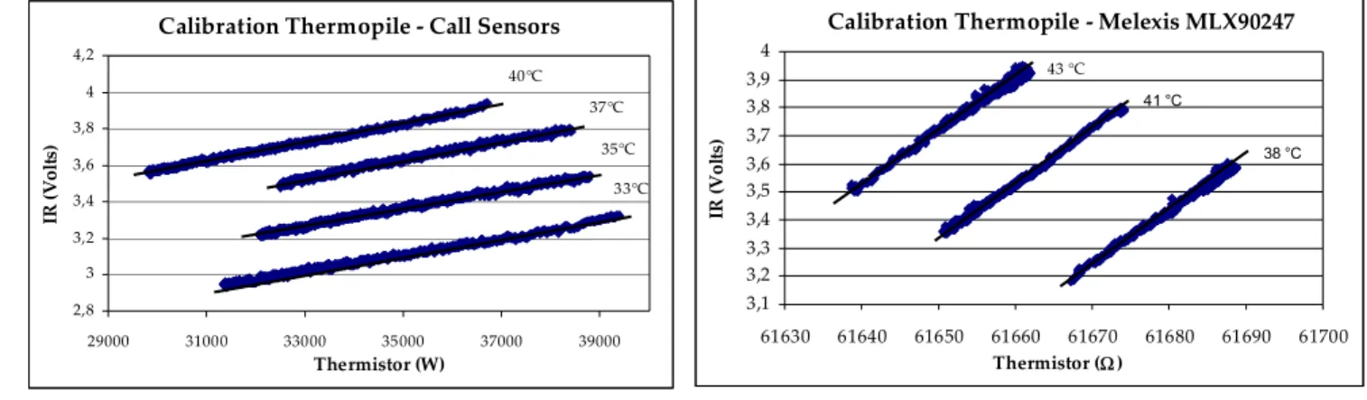
Calibration of the cross sensitivity has been carried out detecting the signal of the thermopile when irradiated only by the radiation of a blackbody (e.g. when it is located directly in front of a wide blackbody, with an area of 20x 20 cm2 , see figure 7) and contemporarily changing the ambient temperature (through the hot air of the air conditioning plant or an auxiliary heat supplier). This operation has been repeated for the following temperatures of the blackbody: for the Cal Sensors TP 30°C, 33°C, 35°C, 37°C, 38°C, 40°C e 41°C, and for Melexis thermopile 35°C, 37°C, 38°C, 40°C, 41°C e 43°C.

The figure 8a and 8b present all the results: it is apparent that all regression lines for diverse black body temperatures present the same trend.

Supposing hence that the slope of the temperature signal versus the cold junction temperature be linear, and equal for the diverse temperatures of the hot junction, the best determination of the slope is carried on through a polynomial multiple regression, supposing the output signal ST be linearly

R4 R3 T1 R2 R1 OP27 C1 T2 IRin Vout

dependent on the resistance of the thermistor RTM , while the dependence on the blackbody

temperature TBB is supposed to be parabolic. That is the following model has been used:

ST= b0+b1RTM +b2TBB+ b3TBB2 (1)

the parameters bi are calculated through a least square multiple regression. Their values and

uncertainties resulted: b0 = -11.554 ± 0.0891

b1 = 4.875 ± 0.0181

b2 = 0.631 ± 0.00502

b3 = (-7.230 ± 0.0689) 10-3

data standard uncertainties 0.019 V

the value b1 represents the desired result. By it the correction of the signal is possible in order to

obtain values independent on the cold junction temperature, and hence on the ambient temperature.

Figure 7: Calibration thermopile with blackbody

Calibration Thermopile - Melexis MLX90247

3,1 3,2 3,3 3,4 3,5 3,6 3,7 3,8 3,9 4 61630 61640 61650 61660 61670 61680 61690 61700 Thermistor (Ω) IR ( V o lt s) 43 °C 41 °C 38 °C

Calibration Thermopile - Call Sensors

2,8 3 3,2 3,4 3,6 3,8 4 4,2 29000 31000 33000 35000 37000 39000 Thermistor (W) IR ( V o lt s) 40°C 37°C 35°C 33°C a. b.

It must be taken into account that other Melexis thermopiles are supplied with a chip able to directly compensate temperature with a chopper system. This automatic compensation has been verified with the same procedure adopted to evaluate the cross calibration just described

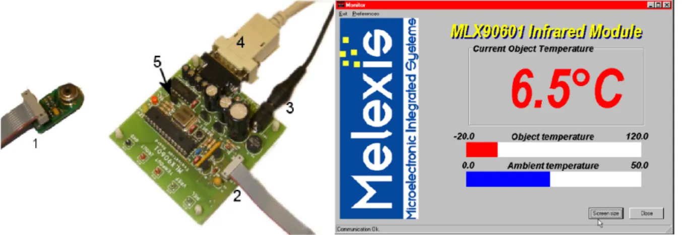
B.3.5 Thermometer module Melexis MLX90601B

General description of this device, its characteristics and performances and reported in appendix 2

B.3.6 Calibration thermometer module Melexis MLX90601B

Calibration of these two devices (thermopile integrated with chip for acquisition feeding and processing) has been carried out with the same procedure above described, i.e. multiple linear regression of thermopile signal versus black body temperature and ambient temperature as measured by the thermistor resistance. Results are reported in fig. 9. It appears immediately that no or little dependence of results on ambient temperature exists, indicating a good performance of the compensation algorithm used by the chip.

Calibration IR thermometerMelexis (2) MLX90601EZA-BAA 0 0,5 1 1,5 2 2,5 3 3,5 0,9 1 1,1 1,2 1,3 1,4 1,5

Ambient temperature (Volts)

IR (V o lts ) 50°C 45°C 40°C Calibration IR thermometerMelexis (1) MLX90601EZA-BAA 0 0,5 1 1,5 2 2,5 3 3,5 4 0,6 0,8 1 1,2 1,4 1,6

Ambient temperature (Volts)

IR (V o lts ) 55°C 50°C 45°C 40°C 35°C a. b.

Figure 9 : Chip Melexis MLX90601B: a. Calibration of chip 1 - b. Calibration of chip 2

Results of the multiple regression are, using again relation (1): b0 = -1131.52 ± 2.654

b1 = (-1.846 ± 0.00411) 10-2

b2 = -0.344 ± 0.00784

b3 = (6.329 ± 0.0951) 10-3

B.3.7 Alternative tests on thermometer module Melexis MLX90601B

Further tests have been carried out to verify the temperature compensation of this chip, sketched in figure 10 a.

Fig. 10 b report the results obtained in the test: output signals of the chip are the thermopile values and the ambient temperature. Thermopile was locate just on the aperture of a blackbody designed and realized by the Heat Transfer and Thermal Measurement laboratory of the University of Rome “Tor Vergata”. Working range of this black body was 30-60°C. The test consists in changing the blackbody temperature and contemporarily perturbing ambient temperature, e.g. directing a heater just on the chip. In fig. 14 b the yellow line is the ambient temperature as measured by a type E thermocouple, and the black one is the signal of the thermistor (in V): clearly they appear strongly correlated. On the contrary the line red (thermopile signal, in V) is correlated to the blue line (type J thermocouple control of the blackbody). As a conclusion, the compensation algorithm provided by the Melexis chip appears quite good.

Control blackbody (tci) Signal thermopile (mis) Signal thermistor (ter) Ambient temperature(tce) S.P

Phon on Phon off

a. b.

Figure 10: Alternative Test: a. Measurement circuit b. Graphic of results

B.4.0 Tests on the pyrometer for measurement of the forehead skin temperature

The optical system is made in order to condense the maximum quantity of infrared radiations in the sensor. Figure 11 illustrates the target distance(from pyrometer 337mm) with an imagine obtained of 20x20m. Sensor Elliptic mirror 52mm 36mm 375 mm Target Infrared radiations 20mm

Figure 11: Operation pyrometer

B 4.2 Pyrometer with thermopile and amplification system

Figure 12 illustrates the pyrometer (see paragraph 4.1) and the amplification system using as thermopile of the Call Sensors firm (see paragraph B.3.4 and B.3.5)

Figure 12 : Pyrometer with thermopile Call sensor

B.4.2.1 Used Instrumentation for measurements

System amplification with battery alimentation

B.4.2.2 Pyrometer calibration

The first calibration tests have been realized by the above described pyrometer, using the Call Sensor thermopile as detector. Tests have been carried out at different distances between blackbody and detector, in order to verify if the pyrometer could give results independent on the ambient temperature radiation. Effectively no difference were found between tests at different distances between 1.3 m and 0.3 m .

Results of multiple regression on tests with variable ambient temperature, using the same equation previously applied are:

b0± sb0= -2.653 ± 0,0396

b1± sb1= (1.396 ± 0,00133) 10-4

b2 ± sb2= (-6.22 ± 0,221) 10-2

b3± s b3= (3.809 ± 0,0319) 10-3

prevision uncertainty of data = 0.0209 V the calibration results are reported in figure 13

Calibration Pyrometer with thermopile Call Sensor 2 3 4 5 6 22000 24000 26000 28000 30000 32000 34000 36000 Resistance (Ω) O u t o p a m (Vol ts ) 30°C 35°C 40°C

Figure 13: Calibration results

It must be noted that calibration of pyrometer takes contemporarily into account the effect of both ambient temperature on thermistor and ambient radiation on the detector. In fact the detector is also hit by radiation coming from the inside of the pyrometer body, due to FOV which is wider than the angle subtended from the mirror to the sensor. Besides, also the not perfect reflectivity of the mirror

could increase the influence of ambient temperature radiation on the detected signals. Anyway the cross calibration takes into account all the previously listed factors.

B 4.3 Pyrometer Melexis MLX90601B

The pyrometer with the detector (integrated in an electronic chip) considered the most suited for the applications, as dimensions and versatility, is shown in Fig. 14 (see paragraph 4.1). The represented chip is the Melexis MLX90601B (see appendix 3 for a description of characteristics, performances and working)

Figure 14: Pyrometer Melexis MLX90601B

B.4.3.1 Used Instrumentation for measurements

Data Acquisition Systems: National Instruments (NI) DAQPAD MIO16X Dual blackbody source 2600 series –SBIR

DC power Supply 40V/1A-PE1537 Philips IR thermometer module Melexis MLX90601B

B.4.3.2 Pyrometer calibration

The calibration tests have been realized for the pyrometer, using the thermometer module Melexis MLX90601B as detector. Tests have been carried out at change ambient temperature between 17÷26°C with set temperature blackbody at 55 °C and chip, in order to verify if the pyrometer could give results independent on the ambient temperature radiation. the calibration results are reported in figure 15

Figure 15: Calibration chip Melexis

This chip has a working range, supplied by the producer, of 30÷55 °C. Taking into account that the measurement range of the skin is 33÷37 °C, the working range as supplied is too large, resulting in an output lower than 0.5 V. This is the reason why it has been decided to use the other chip (the programmable one).

B.4.4 Pyrometer using programmable Melexis MLX90601KZA-BKA as detector

General description of this device, its characteristics and performances and reported in appendix 4

Figure 16: the Melexis MLX90601KZA-BKA: a. Board connection b. Software for visualising

B.4.4.1 Used Instrumentation for measurement

Dual blackbody source 2600 series –SBIR Evaluation board V2 MLX90601 (Appendix 5)

B.4.4.2 Pyrometer calibration

An overall calibration of the pyrometer has been carried out , taking into account, as previously described, all the sources of influence of ambient temperature (cold junction of the thermopile, too wide FOV of the sensor, and non perfect reflectivity of the gold coated mirror). I.e. the pyrometer has been focused on the black body at variable temperature, and the signal has been recorded trying to keep ambient temperature as constant as possible.

Figure 17 reports the results of these tests. Taking into account that a relationship

S

=f(T

, T

)

exists between the three quantities,

S

T

,

T

Tbb BlackBody Temperature

Ta Ambient Temperature – signal of thermistor

This relationship has been evaluated again phenomenologically by a lest square polynomial (2° order) multiple regression, i.e.

S

= B

+ B

· T

+ B

· T

+ B

· T

+ B

· T

· T

+ B

· T

· T

In order to get the black body temperature from the pyrometer signal and the ambient temperature, the previous equation must be inverted, i.e. :

Spyr = (B4 · Tbb2+B6 · Tbb · Ta2)+( B2 ·Tbb +B5 ·Tbb · Ta)+B1+ B3 ·Ta ; (1.2) 0 = Tbb2· (B4)+ Tbb ·( B2 +B5 Ta+B6 Ta2)+B1+ B3 · Ta – Spyr ; (1.3) (B4) 2 Spyr) - Ta * B3 (B1 B6Ta) (B4 4 -B6Ta) B6Ta Ta B5 B2 ( ) B6Ta Ta B5 B2 ( 2 2 ∗ + ∗ + ∗ + + + ± + + − = BB T 03Ta) -6.2029E -(-0.02986 2 Spyr) -Ta * 7.8578 (128.194 03Ta) -6.2029E (0.02986 4 Ta) 0.4325 (-3.3002 Ta 0.4325 3.3002 2 ∗ − ∗ + ∗ + + ± − = BB T (1.4)

Figure 17: Multiple regression

In Fig. 17 the curves obtained (at different

T

S

T

.

• B1 ±∆B1= 128.19 ± 5.39 • B2 ±∆B2= -3.30 ± 0.41 • B3 ±∆B3= -7.86 ± 0.37 • B4 ±∆B4= -0.03 ± 2.1E-03 • B5 ±∆B5= 0.43 ± 4E-02 • B6 ±∆B6= (-6.2 ± .84) E-03

with a prevision uncertainty of data of 0.081V, and a corresponding temperature uncertainty of 0.15°C.

B.4.5 Pyrometer preliminary tests

Preliminary test on the pyrometer are shown in fig.18. The radiation source (forehead skin of several people, as the one in figure) has been placed between 375mm to 400mm, and according to the optical design , the detected area ranged between 20x 20 mm2 and 25x25 mm2. Anyway it was possible to detect the forehead skin temperature.

Figure 18: Preliminary test

B.5.0 Experiments inside the vehicle

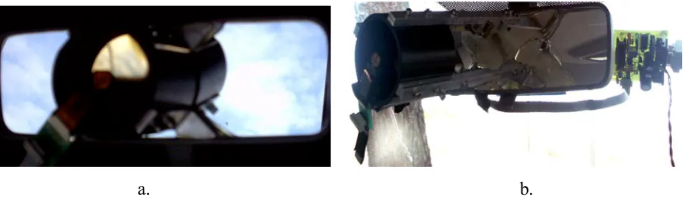
When the pyrometer was mounted on the rear view mirror, it appeared immediately that the working distance declared by the Fiat Research Centre was not suited to the car under test (FIAT Nuova Panda). So it was necessary to mount the device 10 cm far from the mirror, by means of suited extension bars (Fig. 19). A distance of 475 appears more suited to the effective driving style of the major part of drivers.

a. b.

B.5.1 Used Instrumentation for measurement

Circuit for alimentation in the car Evaluation board V2 MLX90601

B.5.2 Experiment results in winter

Winter experiments have been carried out with a group of people of different sex , during the month of February in the following conditions:

Figure 20: Test Fiat Nuova Panda

• Used vehicle: Fiat Nuova Panda version 2004 (kindly put at disposal by the FIAT agency in Rome, ROMANA Auto, owner Prof. Tavernese)

• Pyrometer installed on the rear view mirror of vehicle (Fig. 19)

• Sample of 18 people (13 men and 5 women)

• Calibration range of the programmable chip Melexis MLX90601KZA-BKA , for forehead temperature: 30-40°C

• Working temperature range of the pyrometer (different from the previous value as suggested by the Melexis testing procedure): temperature forehead (33.5 to 38.5°C) ; ambient temperature range as measured by the thermistor: 0°- 40°C

During the winter 2004 different comfort conditions aboard of a vehicle were tested on a group of people instructed to give an information of their hot-cold feeling according to the Fanger list (-3

very cold to +3 very hot, 0= neutral). Changing the inside temperature using the manual air conditioning regulation, the driver gives a personal judgment inherent the felt comfort expressing a vote between +3 and -3. This would result in the so called DMV (declared mean vote)

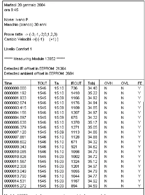
For each vote expressed by the driver all information, shown in figure 21, are recorded by the pyrometer for 15 consecutive seconds. It is also possible to set this recording time for longer time. The range time that elapses between cooling/heating of the vehicle and the following cold/hot sensation felt by the driver, defined acclimatization, could be a problem. In fact the battery level of the laptop (Pentium IV) is limited to 50 minutes maximum and it is possible to make only two tests for each person. Another drawback could be the traffic density in Rome during the tests and the great number of the data that the Melexis EEPROM sends to the laptop.

During the working of the Melexis program (figure 21), the ambient temperature, labelled with Ta

the acquired data and forehead temperature of the driver, labelled with Tobj, are continuously sent to

the computer and visualized. The acquisition card makes an auto-check to verify that everything works well (confirmed by what is written at the end of the data file, see Fig. 21).

Even if during the test time (15 s) Ta could be considered , Tobj can change(for example in a test it

varied between 34.32°C and 35.22°C).

This variation of recording demonstrates that it is very important that the driver forehead should be steady. But this request is impossible for a good and safe driving. In fact the thermopile during the motion of the driver head detects the emission from any parts of the its face: the nose, with a temperature lower of 3°C compared to the forehead temperature [13], or from the eyes whose temperature is very near to the internal one. Besides, eye temperature of people wearing glasses results much lower.

A possible ideal control system [17] could involve a device for objective following (in this case represented by the forehead of the driver) or an algorithm that takes in account only data with highest values, corresponding to the correct pointing of the pyrometer.

Figure 21: Results data

To avoid this trouble in our tests the driver has been forced to drive in straights and without difficulties roads. Moreover during the data elaboration ( see figure 22) only data in a defined temperature range were taken into account. In evaluating the mean forehead temperature, only the values that didn’t change more than 0.3°C one each other about are counted.

A first filtering of data is carried on: for instance in Fig. 22 an ideal range, between 34.8°C and 35.1°C, is considered.

Filter of data 34 34,2 34,4 34,6 34,8 35 35,2 35,4 35,6 0 2 4 6 8 10 12 14 Time (s) F o rehead t em p erat ure( °C )

Figure 22: Filtering of data

First acquired data are processed with equation 1.4 in order eliminate the avoid ambient temperature influence. Than different plot have been shown in order to search a correlation between variables. From the analysis of all data, for the winter case, the following consideration can be deduced:

• Analysis of the declared medium vote (DMV) vs ambient temperature: in figure 23 the positive trend is evident, indicating an increment of the DMV as the ambient temperature increases. This is a trivial result, because logically the perception of very hot to very cold depend from ambient temperature. But the shown results indicate also the spreading of data about this correlation

Ambient temperature vs DMV y = 0,4832x + 17,984 R2 = 0,29 14 15 16 17 18 19 20 21 22 23 -4 -3 -2 -1 0 1 2 3 4 DMV A m b ien t t e m p er at u re (° C )

Figure 23: Ambient temperature vs DMV

• Data of the forehead temperature versus DMV (Fig. 24) don’t show any trend, that is it is not possible to evidence any correlation between DMV and forehead temperature.

Forehead temperature vs DMV y = 0,1054x + 34,094 R2 = 0,0321 31 32 33 34 35 36 37 -4 -3 -2 -1 0 1 2 3 4 DMV F o re h ead t e m p er at u re ( °C )

Figure 24: Forehead temperature vs DMV for winter tests

• No dependence of the ambient temperature on the forehead one(see figure 25), is verified.

Forehead temperature vs ambient temperature

y = 0,1115x + 32,093 R2 = 0,029 31 32 33 34 35 36 37 14 16 18 20 22 Ambient temperature (°C) F o re h ead t e m p er at u re (° C )

• The correlation between the ambient and the forehead temperature does not exist even at constant DMV (e.g. in figure 26 the same behaviour is reported with DMV=0, but the same condition happens for all the other DMVs).

Forehead temperature vs Ambient temperature for DMV=0 y = 0,0844x + 32,61 R2 = 0,0163 32 32,5 33 33,5 34 34,5 35 35,5 36 36,5 14 15 16 17 18 19 20 21 22 Ambient temperature (°C) F o reh ea d t em p erat u re (° C )

Figure 26: Skin temperature vs. ambient temperature at DMV=0(comfort)

B.5.3 Experimental results in summer

Other experiments have been carried out during summer on a different group of people, with different sex. Tests were carried out during the month of June 2004, which resulted particularly hot. In the following, the characteristics of the performed tests are listed:

Figure 27: Test Fiat Punto

• Used vehicle: Fiat Punto Multijet version 2004 (from Romana Auto)

• Pyrometer installed on the rear-view mirror of vehicle

• Sample of 20 people (14 males and 6 femmes)

• Calibration of the programmable chip Melexis MLX90601KZA-BKA: 25-40°C (forehead temperature)

• Pyrometer working range (different from the previous value as prescribed by Melexis test procedure); forehead temperature: 30 to 38°C and ambient temperature: 0°- 40°C.

As a first consideration, the flux of the air conditioning system caused an effect in the skin temperature: when the skiing is invested by the air flow, the transpiration increases. Hence the test has been realized in two different conditions: with the air flux directly in the face of the driver or in upward direction.

• Both in the case when the air is in the upward direction, toward the compartment ceiling (figure 28a), and when the flux air is directed in face of the driver (figure 28b), no correlation between the DMV and the forehead temperature was found. The same situation as the winter case resulted.

Forehead temperature vs DMV with air conditioning in the face

y = 0,1093x + 34,028 R2 = 0,036 31 31,5 32 32,5 33 33,5 34 34,5 35 35,5 36 36,5 -4 -3 -2 -1 0 1 2 3 4 DMV F o re h e ad t e mp er at u re °C Forehead temperature vs DMV y = 0,1227x + 34,288 R2 _{= 0,0369} 31 32 33 34 35 36 37 38 -4 -3 -2 -1 0 1 2 3 4 DMV F o re h ead t e mp er at u re ° C a. b.

Figure 28: Summer results: a. Forehead temperature b. With air conditioning

• Contrarily to the winter case, in the summer case a correlation between forehead skin temperature and ambient temperature can be found. Clearly this correlation must be searched only at fixed comfort feeling. Fig. 29 shows this condition for DMV=0 (comfort condition). Similar results have been obtained in both cases: with air flux on the driver face and without.

Forehead temperature vs ambient temperature DMV=0 y = 0,3791x + 26,824 R2 = 0,3018 32,5 33 33,5 34 34,5 35 35,5 36 36,5 17 18 19 20 21 22 23 Ambient temperature F o rehead t emperat ure( °C )

Figure 29: Skin temperature vs. ambient temperature at DMV=0(comfort)

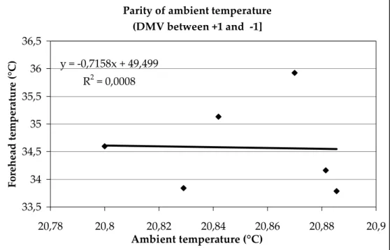
(e.g. figure 30). The example reported in the figure was carried out at a ambient temperature ranging between 20.8°C and 20.9°C. The same consideration holds for all the made tests.

Parity of ambient temperature

20,78 20,8 20,82 20,84 20,86 20,88 20,9 -1,5 -1 -0,5 0 0,5 1 1,5 DMV Am b ie n t tem p er atu re(°C )

Figure 30: Dispersion of DMV at almost equal ambient temperature.

• Also for what concerns forehead temperature, at quasi constant ambient temperature a dispersion appears of about 3 °C, always with DMV ranging from –1 and +1.

Parity of ambient temperature (DMV between +1 and -1] y = -0,7158x + 49,499 R2 = 0,0008 33,5 34 34,5 35 35,5 36 36,5 20,78 20,8 20,82 20,84 20,86 20,88 20,9 Ambient temperature (°C) F o re h ead tem p er atu re (°C )

Figure 31: Forehead vs ambient temperature, at quasi constant ambient temperature, with (DMV between -1÷+1)

B.5.4. Affinity and difference between winter and summer tests

Naturally the mean ambient temperature in the vehicle changes according to the season.

Comparing data in figures 24 and 28, both in comfort conditions, the average value of forehead temperature results about 34°C in winter, and . 34.4°C or 34.2°C.in summer without or with air in the driver face.

Therefore this test demonstrates that the temperature of the skin of a person, subjected directly to external air currents, is function of the air flux. This effect has been studied (in 1992) by Japanese researchers (for example Taniguchi, Aoki and Tanaka [7]) which estimated the temperature variation on the lay simulating the skin of a manikin subjected to strong hot/cold air fluxes with velocities that reached 60 Km/h.

After these considerations, the average forehead temperature can be considered quasi constant at a value of 34°C. Note that this temperature is some degrees lower than the rectal one (internal body temperature) that in general is considered about 37°C (this value is reported in figure 1 in the appendix 1, Fig. 1).

From the data analysis. we notice that there is not a correlation between the skin temperature and comfort level, and it is not possible to establish a general rule, at least taking into account the number of the examined people.

Naturally there is a correlation between the comfort level and the ambient temperature in which the driver is living.

A peculiarity in the relation that links the Ta with Tobjon equal DVM is highlighted analysing the

recorded data. While in summer tests there is a good correlation between the two temperatures (Tobj

increase with the growth of Ta) in the winter tests this correlation disappears.

To explain this it is necessary to consider that the human body releases heat through the effective thermal exchange and the perspiration.

As mentioned in the introduction, the fundamental elements to give an interpretation to this behaviour are:

• The ∆T = Tobj- Ta;

• The skin transpiration that improves the heat release.

• The vasoconstriction that happens when the ∆T is enough high, and decreases the temperature of skin in in winter

• The vasodilatation, which increases the skin temperature increasing the heat transfer to the air, if air temperature is lower of the body temperature.

It is necessary to note that in the winter we have to consider the thermal resistivity of the clothes Icl also to perspiration, while in summer the body surface is more exposed to the air. In summer Icl is equal to 0.5 [1] (this value could increase if the person sweats) , that is the clothes are lighter and both the transpiration and the thermal heat transfer takes advantage [19]. That results in an efficiency in increasing heat transfer from the body to the air with increasing the skin temperature, at least till when skin temperature is higher than air temperature.

In winter the body exposition is reduced, and the Icl is between 1 and 2 for temperate weather [2]. In this case the transpiration is obstructed, because of the thickness of clothes. Consequently the thermal heat transfer is more difficult, and the automatic self regulatory system of body temperature searches for methods of increasing heat transfer different from skin temperature increasing, i.e. sweating.

Another parameter taken into account is the direction of cold-hot feeling versus time. If a value of – 1 is given to this direction, with the meaning of temperature decreasing, and +1 is given to the temperature increasing, all data of Fig. 24 can be divided in two parts, one with direction +1 and the other –1. One could expect that a thermal inertia of the human body could influence results, so dividing data according to this parameter should result in an improving of correlation between skin temperature and DMV. This has been made in Fig. 32 and 33. But again no correlation was found, in both cases. Condition comfort +1 y = 0,1709x + 33,941 R2 = 0,0478 31 31,5 32 32,5 33 33,5 34 34,5 35 35,5 36 36,5 -3 -2 -1 0 1 2 3 4 DMV F o re h ead te m p er atu re (°C )

Condition comfort -1 y = 0,1786x + 34,292 R2 = 0,0439 31 32 33 34 35 36 37 -4 -3 -2 -1 0 1 2 3 DMV F o re h ead te m p er atu re (°C )

Figure 33: Forehead temperature vs DMV for comfort -1

Moreover, it is necessary to stress that every man is different from each other, reacting differently in different situations, and this is the reason why a big dispersion exists even when some correlation is found. No differences were found between men and women, in agreement with Fanger experiments. In general it is believed that a woman feels cold more than a man, but this depend uniquely from the lighter dresses generally worn by them (lower value of Icl). The general Fanger theory is reported in appendix 1.

Taking into account that a not particularly stressed driver has M=1.5 , i.e. 75 W/m2 , if there is no heating loss due to evaporation and sweating (indicated with E+RES ), heat transfer for radiation and convection must be equal to 75 W/m2 approximately. In the case of temperature increasing anyway evaporation increases, either for transpiration or sweating, and a further term must be taken into account. But, as already said this is very much influenced by the cloth thickness, and a more detailed explanation of the obtained results should take into account all the possible phenomena happening at and through the skin.

B.6.0 Conclusions

From the obtained results, we can notice the importance of the environment in which this test was developed, i.e. vehicle. In fact the conditions inside the vehicle are rarely well controlled. For example the mean radiant temperature can be highly different by the air temperature, some anomalous fluxes of air can be enter through the windows or from the air conditioning system, and

Up today the automotive industries build cars equipped by high-technology devices to increase the comfort level of the driver. Nevertheless the vehicle characteristics always introduce the climatization problems described before.

Moreover the control of these parameters is complicated by other conditions as the difference of thermal and ventilating charges to which the vehicle is subjected and in some way the results obtained by tests cannot describe the real situation.

In this work a system to appreciate the individual answer of the tested people is carried out to measure the forehead temperature of each person using a low-temperature pyrometer.

The first experimental test have demonstrated that is possible to measure the surface temperature of the face skin of passengers in the vehicle with an accuracy of 0,15°C.

During the test we found some different problems to be solved:

• The difficult in aiming the pyrometer given by the continuous movement of the head and vibrations of the mirror, even if the level of damping of the Fiat cars tested was good;

• The deposit of pollution on the elliptic mirror of the optical system;

• The restricted range in which the thermal sensor can be used (only due to the electronic card used, as supplied by the manufacturer);

• The sensibility of the thermopile also to the temperature of the pyrometer body, due to its field of view (FOV).

Strength and advantages of the system are:

• The capacity to realize measurements without contact with the measured body;

• The satisfactory velocity response during measurement (about 0,3s);

• The little obstruction in the passenger compartment. In the tests carried out this has caused problems to the visibility of the driver, but find a more suited adjustment is only a problem of industrialization.

When the instrument is not used on black bodies, as the skin, the emissivity ε of the tested surfaces must be known.

In conclusion, the experimental tests performed show that the forehead temperature of the passenger compartment in a moving vehicle are not correlated with the declared comfort vote by the occupants.

Different authors [2,7,11,13,14,16] discussed about this correlation for people living in a normal room, and found that in some cases this correlation exists. Evidently the passenger compartment in the vehicle presents extreme conditions that can invalidate the control.

If the conditions would be controlled in a more accurate way (i.e. reducing or eliminating infiltrations, distributing more homogeneously the flux of air and lowering the difference between wall and air temperature), a correlation could be found.

In the present work, also the differences in winter and summer correlation between skin and ambient temperature have been verified, at equal comfort conditions. This correlation exists only in the summer tests, where the clothes are lighter and more skin is directly exposed to air, and an increase of skin temperature results efficient for preservation of the thermo hygrometric comfort. Contrarily in the winter case the same mechanism is not effective because of the reduced skin surface exposed in the air. This limits the possibility to the thermoregulation system of interviewing, and in this case only like evaporation (transpiration and sweating) that increase heat transfer from skin to air.

The instrument anyway could be profitably used for other applications, in the field of skin temperature measurements, and again in the following conditions:

• focal distance between 375mm and 400

• temperature range: between 30 to 40°C

• skin emissivity from 0.97 to 1 (similar to a perfect blackbody)

These application could be for example the control of people passing through gates of airports, in order to discover the presence of hyperthermia (fever), which is often correlated to particular diseases as SARS or infection from Ebola virus. Or continuous monitoring of forehead temperature of patients in reanimation or intensive therapy departments.

D. INDEPENDENT SENSOR OF TEMPERATURE, RADIATION AND AIR

VELOCITY

C.0.1 Introduction

The thermo hygrometric comfort condition (i.e. experience of hot or cold) depends on four ambient variables: air temperature, mean radiant temperature, air velocity and relative humidity. Commercial instruments for estimating a global feeling of comfort are available, based on thermal balance in systems simulating the skin behaviour, or simple gauges for measuring separately the four quantities. Goal of the present work was to design, realize and test a single instrument able to measure independently during the same test three of the four quantities, which have major influence on the comfort sensation: air temperature, mean radiant temperature and air velocity.

Besides, a portable device is desired, which could be adapted as a medallion on the suit of test drivers of vehicles, in order to give an estimation of the thermal comfort conditions in the passenger compartment.

C.1.0 Studied cases

Three different approaches to solve the above described problem have been followed. The progression of the research was due to improve the resolution of the studied sensors to the wanted quantities.

Initially A single metal wire was studied (see figure 34 a ), because a heated metal wire is a very good detector of air velocity (e.g. the hot wire anemometer). Successive tests and theoretical evaluation showed its inadequacy to detect mean radiant temperature (Tmr). So a flat sensor (PT100

temperature flat sensor) was tested (Fig. 34 b) : a difference at different Tmr was found, bat again

not so high to guarantee a good measuring device, likely due to the small sizes of the sensor (3 mm x 7 mm). Finally it was decided to develop one other sensor by the Heat Transfer Laboratory of The dept. of Mechanical Engineering of the University of Rome “Tor Vergata” , with the help of the Electronic Dept. of the same University (Pro. D’Amico) and the Microsensors Laboratory of the CNR, Research Area of “Tor Vergata” (Mr. Petrocco). In Fig. 34 c this sensor is depicted: it is much wider (25 mm x 50 mm)

a. b. c.

Figure 34: studied cases: a. nickel wire b. PT100 c. detail of the flat sensor gold

C.2.0 Nickel wire

A nickel wire with diameter 0.7mm (see fig. 35) , can easily measure ambient temperature when not heated, and air velocity if heated to a defined temperature. The present tests were carried out to recognize if it was possible to measure also mean radiant temperature.

Recognizing the mean radiant temperature has been evaluated by comparing the difference between steady state r transient data of the sensor, when it is bright or blackened with a painting at high emissivity (e.g. a opaque black painting, of colloidal graphite, Aquadag, which both present generally emissivity higher than 0.95).

Figure 35: Nickel wire

C.2.1 Important considerations in measurement preparation.

A special configuration was adopted to carry on measurements on nickel wire: the wire was stretched within two cooper wires in V shape (see figure 36). These two holders have three purposes: the first to sustain the wire, the second to stretch it avoiding its relaxation during heating,

and the third constitute a four wire resistance meter, leading the current by two of them (at opposite sides) and detecting the voltage drop by the other two.

Nickel Wire

Copper

Connections

Figure 36: Configuration of the nickel wire

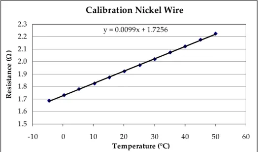
C.2.2 Calibration curve for the nickel wire

Before measurements, the nickel wire must be calibrated in order to detect the relationship between its electric resistance and temperature.

This calibration is carried on changing the temperature of the wire (measured in a calibration bath by a Platinum resistance thermometer PRT-25, standard of the laboratory), and contemporarily measuring the wire electrical resistance with four wire technique (Kelvin bridge) as above mentioned. Fig. 39 represents a sketch of the calibration set up.

During calibration the nickel wires are positioned around the tip of the platinum resistance thermometer (PRT-25), and inserted into a properly realized comparator ( a glass pipe with an inlet and outlet of the liquid coming from the thermostat, i.e. a mixture of 50% distilled water and 50% ethylene glycol; Result of calibration is the relation between electric resistance and temperature of wire. D a ta A c q u is itio n S y s te m T h e r m o s ta t (H2O + G lic ol) N ic k e l W ire s P T R -2 5 C o n tro l

C.2.2.1 Instrumentation used for calibration:

2700 Multimeter/Data Acquisition Systems -Keithley Integra series

Platinum resistance Thermometer (PTR-25) standard, calibrated by IMGC – CNR (national metrological laboratory, Torino, Italy)

Thermostat -Julabo F33

Instrumentation used during tests:

Data Acquisition System National Instruments (NI) DAQPAD MIO16X Bipolar Operational Power supply/Amplifier –Kepco BOP100-1M 100V/1A Standard resistance (manganine shunt) 0.1Ω

C.2.2.2 Calibration results

The nickel wire presents a linear behaviour between resistance and temperature, at least in the temperature range investigated (-5°C÷55°C). As a result also the sensitivity

R T ∂

∂ _{= 0.392°C/Ω has} been obtained, with standard uncertain Sy/x=1.6 10-3Ω. In figure 42 the calibration of the nickel wire is reported.

Calibration Nickel Wire y = 0.0099x + 1.7256 1.5 1.6 1.7 1.8 1.9 2.0 2.1 2.2 2.3 -10 0 10 20 30 40 50 60 Temperature (°C) R e si st a n ce ( Ω )

C.2.3 Description of the experimental set up for transient test on nickel wires (Fig. 39)

Through the DAC function of the data acquisition system (with an output variable between 0 and 10V), the power supply is commanded to give a constant current variable in the range 0÷1A. This power is used to feed the circuit constituted by the wire and the shunt resistance in series.

At the beginning the DAC signal is set to send a bias current of 10mA for a time interval of 5s. This negligible current is enough to detect the resistance of the wire, without increasing its temperature by self heating. After this stationary first step, an increase of the DAC output is given to the power supply for an interval of 15 s. In both tests the If register the shunt and nickel wire voltage drop is recorded, and the wire resistance is evaluated by the following relation:

Shunt Shunt Wire Wire V R V R = . (2).

Temperature of the wire is obtained from its resistance by means of the performed calibration.

Figure 39: circuit for test nickel wire

C.2.4 Nickel wire results

Both free and forced convection were tested on wire, the first protecting the wire with transparent case (Fig. 40 a and 41b), and the second investing the wire with the air flux from a fan.

The results of the experiments in free convection also with air conditioning are reported in the figure 41a . The temperature behaviour represented is influenced by a overshoot in voltage, likely

due to a retard in developing natural convection, and hence a major temperature increasing a the beginning of heating.

Resistance wire Nickel

2.1 2.12 2.14 2.16 2.18 2.2 2.22 2.24 0 50 100 150 200 Time (s) R esi st a n ce ( W ) a. b.

Figure 40: wire nickel: a. forced convection b. Behaviour of the wire nickel

.

Natural convection with air conditiotining

2,18 2,19 2,2 2,21 2,22 2,23 2,24 2,25 2,26 0 50 100 150 200 250 Samples Re si st a n ce (Ω ) Forced convection 2,22 2,23 2,24 2,25 2,26 2,27 2,28 2,29 2,3 2,31 0 50 100 150 200 250 Samples Re si st a n ce ( Ω ) a. b. Figure 41: test nickel wire: a. Natural convection b. Forced convection

C.2.4 Theoretical temperature versus time behaviour of the wire.

The theoretical trend of temperature of wire during heating can be estimated a priori by the simple solution of a lumped parameter problem, balancing the three heat fluxes involved in the description of the phenomenon. These three fluxes are: Q& , heat produced by the current flow into the wire; ₁ Q& ₂ variation of the internal energy of the wire during heating, and Q&₃ thermal heat transferred to the ambient air by convection.

3 2

1 Q Q

Q& = & + & (3) ∴ 2 1 RI Q& = (4) dt dT mc Q w p = 2 & (5) Q&3 =hAw(Tw −Ta) K m W ] [h = ₂ (6) where:

R- wire average electric resistance; I-electric current; h the convection coefficient (free or forced).; Aw-wire external surface; Tw- wire temperature, Ta- ambient air temperature

If h is considered independent on temperature, the above written balance constitutes a first order linear differential equation that can easily be solved, leading to the relation

          − + = −mc t hA w a p w e hA RI T t T( ) 1 2 (7)

h values are influenced by the phenomenon governing heat transfer: ! in free convection     ∆ ∝ ⇒ ∆ ∝ ⇒ − = 1/₁4_/3 flow Turbulent flow Laminar ) ( T h T h T T f h _{w a}

! in forced convection h is dependent on air velocity w, as predicted for example by the empirical correlation (e.g. the one of Eckert and Drake)

) Re 5 . 0 43 . 0 ( Pr0.38 + 0.5 = Nu (8)

which leads to the following values

    = = m/s 5 and convection forced for K W/m 500 convection free for K W/m 200 ) ( ₂ 2 w w f h

! when radiation is present, a radiation component of the convection coefficient hr can be

evaluated according to the following relations:

(

)

(

)

(

)

(

)

(

)

Fig. 46 b reports the computed temperature behaviours for three different air velocity, i.e.

s m . ; s m ; s m w=5 1 02 .

When radiation is taken into account, it can be computed that the radiation component hr assumes a

value about 6 W/m2K, influencing only 3% of the value of natural convection. This is the reason why this system (the wire) is a very good tool to evaluate the ambient temperature and the velocity

of air, but is influenced very little by the mean radiation temperature. The measurement of this last hence must be carried out by other techniques. The reason of the negligible amount of the hr as

respect to convective part of h is related to the high values of h in the case of convection as computed by the empirical relations. Really, it is not hr to be very small (its value is about the same

of flat surfaces) but hconv to be hugely high for wires.

Experiments carried out with two wires, one bright (without coating) and the other covered with a black painting, didn’t show any difference in h, confirming the negligible amount of hr .

This is the reason why further experiments were carried on flat surfaces.

3 2 1 Q Q

Q& = & + &

2 ) (T T RI hA dt dT mcp w+ w w− a = ) ( 3 hAwTw Ta Q& = − dt dT mc Q w p = 2 & 2 1 RI Q&= τ TW 1 TW2 TW3 Ta Ta (5 ms) (1 ms) (0.2 s) T t a. b.

Figure 42: Theoretical behaviour of the wire: a. Theoretical trend of temperature b. Behaviour air velocity

C.3.0 PT100

As a first trial, a two flat PT100 was tested, again one as supplied by Centro Ricerche FIAT (see fig. 43), and the other insulated (in order to avoid short circuit inside the Pt winding) and blackened. Sizes of the devices were 7x3 mm2-(rectangular shape), and 1mm thickness, with the platinum on the upper flat surface.

Figure 43: Flat PT100

C.3.1 Important considerations for measurement preparation

In order to put into evidence as possible the differences between the two sensors (the bare one and the blackened) an accurate resistance measurement must be made. This is done with the four wire resistance. Two couples of leading wires have been tin soldered to the connection of the PT100, (see figure 44), getting the two current and the two voltage terminals of the resistance. In order to increase the radiation effect, the two sensors were both glued to an aluminium base (30 x 60 mm2), one blackened together with the sensor.

Figure 44 Blackened and bright PT100

C.3.2 Used device

Data Acquisition System: National Instruments (NI) DAQPAD MIO16X Bipolar Operational Power supply/Amplifier –Kepco BOP 100V/1A Standard resistance (shunt) 0.1Ω

C.3.3 Description of the experimental set up (Fig. 45)

Through the DAC of the acquisition system, a voltage signal (0-10V) is sent to the power supply, which respond with current in the range 0÷1A. Also in the present case, at the beginning the two sensors are fed with a low current bias (10mA) for five seconds. Then the DAC voltage is increased to 60mA for 15 seconds The voltage drop on the on the shunt and PT100s are recorded by the data acquisition system, and the PT100 resistance is evaluated again by the following relation:

Shunt Shunt PT PT V R V R 100. 100 = (11)

Temperature is obtained with a standard relation between resistance and temperature, as supplied by international rules (e.g. ITS90)[15]. Only a check of the 0°C resistances of the sensors were measured.

C.3.3 PT100 results

As a result of the tests, a first difference between the blackened and the bright PT100 was obtained. Both a curvature change in the temperature behaviour between the two sensors (the bright one and the blackened one) and a difference in asymptotic temperature was noted, demonstrating a variation of the convection coefficients, and hence of their radiation component. In figure 46 the results of the two PT100s (blackened and bright.) are reported, and the above mentioned differences are evident.

PT 100 Blackened 107 108 109 110 111 112 113 114 0 200 400 600 800 1000 1200 1400 Samples R e si st a n ce ( Ω ) PT 100 Bright 104 106 108 110 112 114 116 0 200 400 600 800 1000 1200 1400 Samples R e si st a n ce ( Ω ) a. b.

Figure 46: Results PT100: a. Blackened b. Bright

C.3.4 PT100 Behaviour

Most of the considerations made about the Nickel wire can be repeated at the same level for the PT100s. But now the radiation component of the convection overall coefficient cannot any more be considered negligible, and influence thermal behaviour as described.

From the experience of these tests, it has been decided to built a new type sensor, constituted by a bigger flat surface, with a metal coating to detect temperature and to lead current in order to be heated. Again transient behaviour is considered quicker and more accurate to evaluate convection coefficient, because of lack of anomalous natural convection behaviours, even in steady state.

C.4.0 Flat sensor

As previously said, it has been decided to develop new comfort sensors, flat and enough wide to avoid the edge effect (as in the case of wire), in order also to amplify the differences between bright and blanked sensing elements noticed on the PT100s.

The principal characteristic of the new flat sensor realized are:

! double nature (it is divided in two parts: a blackened and a bright part),

! dimensions of a medallion, with an area of 250mm2, each part 25 mm x 50 mm;

! the sensible element is a deposit of conducting metal (gold or platinum), insulated from the substrate; with a resistance enough low (5-10 ohm) to allow good voltage drop

measurements with the usual data acquisition systems.

C.4.1 Mask computing and design

The double sensor must be wide enough to don’t be influenced by the size effect (as the wire), so a total size of 50 x 50 mm2 was chosen (one half for each part, bright and blackened). Besides it must have a bifilar winding, in order to reduce the inductance and consequent ambient electric noise. In order to have an enough low resistance, only few double pass were designed. The complete description of the two version of the sensor (gold and platinum deposit) is reported in the following: Gold deposit (Fig.47):

Path for soldering : 5mm Path width =4mm

Separation between paths =0.18mm Separation between sensors= 0.20mm Total average length (L)= 299.99mm

Figure 47: Mask for gold deposit Platinum deposit (Fig.48):

Path for soldering : 5mm Path width =6mm

Separation between paths =.25mm Separation between sensors= 0.5mm Total length (L)=201.5mm

The Sensor with the platinum deposit has been designed with a wider track, because of the higher electrical resistivity of this material, compared to the gold one.

In the following the resistances of the two obtainable sensor have been calculated, assuming the resistance of the deposit equal to the bulk material one, even if it is well known that this seldom happens.

Notation:

Cross section of the deposit: S= r*l where r thickness e l width; δ density R=ρ*L/S where ρ= resistivity; L= total length of the deposit

For the gold deposit, the above relations give

l =0.004 m; L = 0.2999m; r = 2.5·10-6 Å; δ =2.200·10-8 ;S = 1.000·10-8 Final result for gold coating resistance R = 0.6598Ω

For the platinum deposit, the above relations give

l =0.005 m; L = 0.2015m; r = 2.5·10-6 Å; δ =1.048·10-8 ;S = 1.500·10-8 Final result for platinum coating resistance R = 1.4078Ω

C.4.2 Fabrication process

Fabrication of the flat sensors (gold and platinum deposit) were carried out with the two above described masks, and with the reported thickness, by the CNR Roma laboratory of sensors and microelectronic of the Research Area of Tor Vergata (Prof. D’Amico and Mr. Petrocco)

C.4.2.1 Gold deposit

Gold has been deposited on a normal glass(for windows) substrate, 1.87 mm thick, cut in the shape 70 x 70 mm2.

Process of deposition:

1. Cleaning of the substrate with a soap solution, then with acetone and finally with isopropyl alcohol

2. Spinning: the base, after cleaning with a jet of nitrogen gas, is covered with resist solution 5214, than centrifuged at 4000 rpm in vacuum for 60 s. The resulting thickness of the resist layer after application is 1.5 µm