Computational modeling of fiber reinforced concrete with application to projectile penetration

Corso di laurea in Ingegneria civile

D.I.S.T.A.R.T.

Dipartimento di Ingegneria delle Strutture, dei Trasporti, delle Acque,del Rilevamento e del Territorio

Tesi di laurea in

Progetto di strutture

COMPUTATIONAL MODELING OF

FIBER REINFORCED CONCRETE WITH

APPLICATION TO PROJECTILE PENETRATION

Candidato: Relatore:

Pietro Marangi Prof. Ing. Marco Savoia

Correlatore:

Prof. Ing. Gianluca Cusatis

“Ritorna con il tuo scudo

o sopra di esso”

capacity and durability. Even thought engineers have designed the reinforcement of concrete structures for centuries, concrete material is still not well understood. This statement is particularly true outside the elastic range when fracture and other inelastic phenomena occur. The main reason for this hard behavior is due to the extreme complexity of concrete internal structure that is highly heterogeneous. To overcome this problem, in the past, several model have been formulated using different approaches. In this work, the goal is to study at first the Lattice Discrete Particle Model (LDPM) and then to develop one method that allows to study the FRC.

The LDPM will be extended to include the effect of dispersed fibers with the objective of simulating the behavior of fiber reinforced concrete for armoring system applications. The developed model, named LDPM-F, is validated by carrying out numerical simulations of three-point bending tests on fiber reinforced concrete mixed characterized by various fiber volume fractions. Finally, LDPM-F is applied to the analysis o the penetration resistance of fiber reinforced slabs.

In Chapter 1 the formulation of the LDPM is presented and explained, showing the geometry of the model.

In Chapter 2 the constitutive law for interaction of fiber-concrete is described and explained.

In Chapter 3 an experimental campaign of uniaxial compression tests and three point bending tests on plain concrete specimens are simulated.

In Chapter 4 an experimental campaign of three point bending tests on FRC specimens is simulated and the calibration and validation phases are described, in order to clarify the LDPM-F.

In Chapter 5 the results found in the previous chapters will be used for armoring system applications, in order to predict the FRC response.

Introduction...1

Features of the model...2

Geometrical Characterization of Concrete Mesostructure...4

First step: Number and size of coarse aggregate pieces ...4

Second step: Particle position ...7

Third step: Inter-particle connection...7

Fourth step: facets generation ...8

Discrete Compatibility and Equilibrium Equations...12

LDPM Constitutive Law...17

Elastic behavior...17

Inelastic behavior...18

Fracturing and cohesive behavior ...18

Poor collapse and Material Compaction...21

Frictional behavior...23

Numerical Implementation and Stability Analysis...25

Constitutive law for the concrete-fiber interaction ...28

Introduction...28

Modeling of the single fiber behavior...30

Matrix micro-spalling ...37

Cook-Gordon effect ...38

Two way pullout ...40

Analysis stages...40

Stage 1: neither embedment ends completely debonded ...40

Stage 2:short embedment end complete debonded...41

Stage 3: both embedment ends completely debonded ...42

Parameters analysis of the model...44

Presentation of fiber parameters ...44

Pullout hardening behavior...45

Two way pullout ...46

Debonding fracture energy ...47

Bond strength...48

Snubbing effect ...49

Spalling effect ...50

Numerical analysis plain concrete subject to tension and compression ...56

Introduction...56

Parametric analysis ...63

Three point bending test (3PBT) ...63

Uniaxial unconfined compression test (UC)...67

Calibration stage ...71

Fracture energy control...75

Numerical analysis fiber reinforced concrete (FRC) subject to tension...78

Introduction...78 Phases of pre-calibration...79 Fiber generation ...79 Presentation of parameters...81 Model sensibility...81 Calibration stage ...84 Validation stage ...87

Numerical analysis of projectile penetration for FRC slabs...92

Introduction...92

Geometry of the test...93

Penetration test of concrete slab ...94

Penetration test of FRC slab ...97

Design of Armoring System ...100

Chapter 1

The lattice Discrete Particle

Model (LDPM)

Introduction

Concrete is an heterogeneous material, constituted by three phases, with different property: aggregate, matrix and interfacial boundary. In order to investigate these aspects, a lot of models have been proposed in recent years, but although these allowed us to achieve good results, the concrete feature is not still completely understood. The principal reason of this, is the complexity of the internal structure, that is linked with the length scales of observation used for the model. By this point of view, changing the observation level, is possible to show, different aspects that are directly matched with the heterogeneity of the material. The scale length range from the atomistic scale (10-15 m), characterized by the behavior of crystalline particles of hydrated Portland, to the macroscopic scale (101 m), at which concrete has been traditionally considered homogeneous.

In the last twenty years, several authors, have done materials models that use miniscale or mesoscale, to study this kind of material, in special way for the geological problems.

Miniscale models in which concrete is treated as three-phase composites have been proposed by Wittmann (1988), and Carol (2001). They used finite element technique to model with different constitutive laws coarse aggregate pieces, mortar matrix, and inclusion-matrix interface. Another remarkable study is done by Van Mier and coworkers (1992), they proposed a model realized with finite elements but without continuum hypothesis. Concrete was modeled through a discrete system of beams. Important is also the experience by Bolander (1999), which realized a discrete miniscale model based on the interaction between rigid particles obtained though the Voronoi tessellation of the domain.

The main advantage of miniscale models is they are able to reproduce realistic simulation of cracking, coalescence of multiple distribution cracks into localized cracks, and fracture propagation. The only problem that affect these kind of model is that they tend to be computationally intensive especially for 3D modeling. Mesoscale models appear because they are computationally less demanding than the miniscale models. For mesoscale model, concrete is modeled by the whole

aggregate pieces and the layer of mortar matrix between them. The technique used is finite element. Some examples are Cusatis et al (2003a,b), Cusatis et al (2006), Cusatis & Cedolin (2006).

Summarizing every thing, the principal difference among these two approaches is that, miniscale model describe the concrete like three-phase material: cement paste, aggregate and interfacial transitional zone, and the length scale is of 10-4 m or less. The mesoscale, is fundamentally different, because this show only the mortar and the coarse aggregate, and the scale order is 10-3 m. Both approaches have the problem, which are very numerically expensive, but for the concrete has been seen that using the mesoscale model, that is relative expensive, and is also possible to achieve fairly good results like the miniscale.

The old models, implemented for macroscale, allowed to obtain good result, but they are not able to simulate material heterogeneity and its effect on damage evolution and fracture. For solving these problems now, one possible manner is to use models, that are able to simulate the concrete at the level of the mesostructure, with discrete approach. In this way, it is possible to replicate damage and fracture, and to capture the phenomena related to the randomness of the material.

Features of the model

The model present in this work, use an analysis at the mesoscale level and is called Lattice Discrete Particle Model (LDPM). It is the result of the union by two different models: Discrete Particle Model (DPM) and Shear Lattice Model (CSL). The principals features of the model are:

a) Concrete mesostructure is simulated by a lattice that match a system of

particles that are in interaction into their through triangular facets. This lattice is obtained by a Delaunay triangulation of the aggregate centers.

b) The specimen is created by a randomly distribution of particles, that is

computed taking in account the basic properties and the granulometric of the aggregate.

c) The geometrical interaction between the particles is obtained by

three-dimensional domain tessellation defining a set of polyhedral cells each including one piece of the aggregate.

d) Two adjacent pieces of aggregates are connected by the generic lattice

element, that transmits shear and normal stresses. These are assumed functions of normal and shear strains. Allotting the displacements the model works, and permit to find the stress field.

e) The stresses act on contact areas which are defined by constructing a

barycentric dual complex of the Delaunay triangulation.

f) Starting from the strains is possible, using the constitutive law to define

the stresses, taking into account the stress-strain boundaries.

g) The constitutive law give the following behavior: softening for pure

tension, shear-tension and shear with low compression and it is hardening for pure compression and shear with high compression.

h) Friction and cohesion are shown into the shear response.

LDPM has inherited from DPM the MARS computational environment that includes long range contact capabilities typical of the classical formulation of Discrete Element Methods (DEM). This feature is particularly important to simulate pervasive failure and fragmentation.

LDPM allows to capture a number of new features that greatly improve its modeling and predictive capabilities. These new aspects can be explained as follows:

1) The particles interaction is formulated by the assemblage of four aggregate

pieces whose center are the vertex of the Delaunay tetrahedralization. This model geometry allows to include into the constitutive law the volumetric effects, that the other models are not able to capture.

2) Each single aggregate is contained into one polyhedral cells that is made

by different triangle facet. Stresses and strains are defined at each single facet. This configuration allows a better stress resolution in the mesostructure, which, in turn, lead to a better representation of mesoscale fracture and damage.

3) The constitutive law simulates the most relevant physical phenomena

governing concrete damage and failure under tension as well as compression. This law compared with the previously existed provides better modeling and predictive capabilities especially for the macroscopic behavior in compression with confinement effects.

The LDPM is able to simulate all aspect of concrete response under quasi-static loading, including tensile fracturing, cohesive fracture and also size effect, compression-shear behavior with softening zero or mild confinement, and high confined compression, and strength increase under biaxial loading. The following sections will explain before the geometrical characterization of the model and then equilibrium equation with constitutive law.

Geometrical Characterization of Concrete Mesostructure

The geometrical structure of the concrete mesostructure is obtained with four divers steps. In these phases the objectives is define:

1) Number and size of coarse aggregate pieces; 2) Particle position;

3) Inter-particle connections;

4) The creation of a surface, into the two adjacent particles that permit to

exchange the forces.

First step: Number and size of coarse aggregate pieces

The first step is to define the particles diameters and the respective number, that will be used for refill the specimen volume, and generate the its surfaces. In this sense, there are different practice to make this in the LDPM, first of all it will compute the particles and then the zero node point, that also will be explain in the following section. However, the first hypothesis is to consider the particles with sphere shape, under this assumption, the concrete granulometric distribution can be represented by particle size distribution function (Psd), proposed by Stroeven:

( )

(

)

[

]

1 0 0 1_{− ⋅} + = q q a q d d d qd d f

where da is the maximum aggregate size and d0 represent the minimum particle

size.

The precedent Psd, can be interpreted as probability density function (Pdf), this will allow to find the percentage associated with a certain diameter, using the cumulative distribution function (Cdf), that is expressed as:

( )

_∫

( )

₍

(

)

₎

− − = = d d q a q d d d d d d f d P 0 0 0 1 1 δ

( )

n a d d d F _⎟⎟ ⎠ ⎞ ⎜⎜ ⎝ ⎛ =

where n= 3−q. For q=2.5, the relation represent the classical Fuller curve extensively used for the concrete. With this curve is possible to check the concrete granulometric, analyzing the percentage of passing in function of the diameter, in this way the concrete quality is guaranteed if this curve is contained into the Fuller range. This technique allows to have the best specimen refill and to avoid the empty space, as showed in the Cusatis (2001).

The specimens used in the simulations have particles created with the 30% of the total curve granulometric (Fuller curve), starting from the coarse aggregate; this allows us to find good results, because the computational cost is lower and at the same time there are not big differences between results found using another percentage of generation.

For simulate the specimen in terms of number and diameters of particles, it is important to know: c = cement content, w/c = water to cement ratio, V = specimen volume, da = maximum aggregate size, d0 = minimum particle size.

The following procedure is used to find and then place the particles inside the specimen volume:

a) Calculate the volume aggregate fraction as v_a =1−c ρ_c−w ρ_w−v_air, where w=

( )

w c c is the water mass content per unit volume of concrete,

3

3150Kg m

c=

ρ is the mass density of cement, _{1000Kg m}3

w =

ρ is the

mass density of the water, and v_air is the volume fraction of entrapped or entrained air, ( usually 3-4%);

b) Compute the volume fraction of simulated aggregate using the following relation:

[

( )

]

[

(

)

n

]

_a a a o ao F d v d d v v = 1− = 1− ₀ ⋅ ;

c) Compute the total volume of simulated aggregate as V_ao =v_aoV ;

d) Calculate the particle diameter by sampling the Cdf by a random numeric

generator:

[

(

q

)

]

q a q i i d P d d d = ₀1− 1− ₀ / −1 , where Pi is a sequence of

random numbers between 0 and 1.

e) The total number of the particles is obtained by checking, for each new generated diameter in the sequence, that the total volume of the generated particles ~

(

3 6

)

0 i

a d

0 0

~

a a V

V > occurs, the current generated particle is discarded and the particle generation is arrested, Cusatis and coworkers (2009).

The graphical representation of the procedure explained before is shown in the Fig. 1.1, whereas in the Fig. 1.2 is represent the computational sieve curve obtained during the generation of a cube specimen characterized by c = 300 kg/m3, w/c = 0.5, d0 = 4 mm and da = 12 mm.

Figure 1.1: Cumulative distribution curve

The diameters and number particles, found in this way, will be used to fill the specimen, now the procedure will be completed creating the zero-diameters particles (nodes), that will be placed over the external surfaces. That practice, is important, for the third step, when the tetrahedral will be generated.

The method used to search the number of surface nodes is the following, assuming that the external surface of the specimen volume can be described with a set of polyhedral face, and that is Le is the generic length of the edge specimen,

and Ap the generic surface area, the number of the nodes will be given by these

ratio L_e h_sand 2

s p h

A , where h is the average surface mesh size, chosen such _s

that the discretization resolution on the resolution on the surface is comparable to the one inside the specimen. This is done using this relation h_s =ξ_sd₀, by numerical experiment which showed that putting ξ_s =1.5 leads to obtain good results. Clearly for each vertex on the external surface will be placed one node.

Second step: Particle position

The particle computed before, will be now placed in the volume specimen, using a random distribution, on vertexes, edges, surfaces, faces and interior volume. The following idea for the ranked, is first of all, set the vertex nodes, and after in the edges and surface created among these vertex nodes, place other particles, by allowing a minimum distance of δ_sd₀ to minimize the geometrical error of the discretization. The typical value used for δ_s =1.1, permit to achieve good mesh. Using a procedure introduced by Bažant, it is possible to generate a statistically isotropic random mesostructure, where the center of particles are placed in the volume of the specimen one by one, from the largest to the smallest.

When the procedure, for generate the particles position, is finished, one control is done, for avoid possible overlaps of this particle with the previously placed particles and with surface nodes. In this phase, at the surface nodes are assigned a fictitious diameter of δ_sd₀ and a minimum distance of d_i 2+d_j 2+ξd₀ among the center of the particles with diameters di and dj is enforced. The value of ζ, is

very important, because it determines the concrete behavior, for ζ=0 or very small values, the particles distribution is not statically isotropic, and present areas where there are low particle density and others zones with high particle density. In the same manner using very large values of ζ, the specimen volume is saturated quickly and not all particles can be positioned. After several numerical experiments, the best value found is ζ = 0.2, using this, it is possible to avoid the volume saturation while leading uniform particle distribution.

Third step: Inter-particle connection

The third step lets to define the topology of the interaction among the particles. This is performed using a Delaunay tetrahedralization, that utilizing the nodal coordinates of the particles center allows to build three-dimensional tetrahedral, which does not overlap, fill all the volume of the specimen. In each vertex of the

tetrahedrals is placed a particle, generated in the first step, and permit to fill the total volume specimen. In this study, the Delaunay tetrahedralization is carried out by using the TenGen code.

Fourth step: facets generation

The last step, the forth has the aim to define the surface through which the forced are exchanged from one particle to another. There are different ideas proposed for describing this aspect of the problem, in previous works, the interaction between the particles were realized by the edge that was created as a strut. It connected the two adjacent particles, and the effective area of this strut was defined by performing a tessellation of the domain anchored to Delaunay tetrahedralization. This approach gives a good result in terms of fracture behavior and also for the concrete failure under unconfined compression. These methods have the lacuna that does not say something about the volumetric effects that are essential for description of the concrete behavior under high confining pressure.

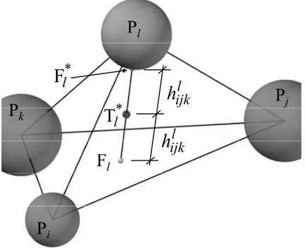
In the LDPM model, the principal thing is the elementary cell, that is the tetrahedral. There be possible, to see this like the union of four sub-domains, where each sub-domain contains one particle, see Fig. 1.7. The single facet of these sub-domains will be the surface, where will be applied the relation to allow the force exchange.

The last phase will be realized for this local geometry for every elementary cell and for each particles. Starting from the tetrahedral, the tessellation will be construction of the following procedure:

a) One point on each edge (edge-point) is defined at midway of the counterpart of the edge not belonging to the associated particles ( point Eij

in the Fig. 1.3 );

b) One point on each triangular face (face point) of the tetrahedron is defined as follows. First points located on the straight lines connecting each face node to the edge point located on the edge opposite to the node under consideration are considered. Similarly to the edge points, these points are located at midway of the line counterpart not belonging to the associated particles. See point F*kl in Fig. 1.4 . Later, the facet point is selected as the

c

P

_i

P

_j

E

_ij

d

_i

d

_j

h

_ij

h

_ij

Figure 1.3: Construction for edge-point

P

_k

P

_i

P

_j

E

_ij *

F

_lk

d

k ij

E

k

ij

h

k

ij

h

Figure 1.4: Construction for face-point

c) One point in the interior of the tetrahedron ( tet-point) is defined by the centroid ( Tl in Fig. 1.5 ) of the points identified, similarly to what is done

for the face points in item 2, on the straight lines connecting each node of the tetrahedron with the face points on the face opposite to the node under consideration ( points Tl* in Fig. 1.5 ). Again, these point are located at

midway of the line counterpart not belonging to the associated particles.

P

_k

P

_i

P

_j

F

_l

P

_l

*

T

_l

*

F

_l

e

l

ijk

h

l

ijk

h

Figure 1.5: Construction for Tet-point

d) Finally, the tessellation of the tetrahedron is obtained by the set of triangles by connecting the tet-point with the one of the edge-points and one of the face-points. Each tetrahedron result tessellated with twelve triangular face ( Fig. 1.6).

This is only one type of tessellation possible, basically different procedure could be realized but numerical experiments show that this is the best for minimize the intersection between the tessellating surface and the particles. Isolating one particle and its facets, a polyhedral cell is obtained.

This is the sub domain that has irregular and also random shape, this characteristic is an important property that ensures a realistic representation of the kinematics of the concrete mesostructure, and it especially allows avoiding the excessive

T

P

_k

P

_i

P

_j

E

_ij

F

_l

P

_l

E

_ik

E

_jl

F

_i

F

_k

E

_il

E

_kl

F

_j

f

Figure 1.6: Tessellation of the tetrahedron.

Discrete Compatibility and Equilibrium Equations

The tetrahedron formed by the basic four-particles, as showed in the Fig.1.7, is the primary element used to derive the governing equations of the model. Every particle, which forms this tetrahedron, is included in a sub-domains Vi ( i

=1,….,4), and all together create the original element. Each sub-domain, has a portion of the three tetrahedron edges attached to the node and also, six triangular tessellation facet joint to the three edges, Fig. 1.8. One of the most important things is to describe, the displacement field in every domain, this is done by rigid body kinematics.

a

x

₃

x

₂

x

₁

P

_i

u

_i1

θ

_i1

u

i2

u

_i3

θ

_i3

θ

_i2

C

_k

V

_i

Figure 1.8: Sub-domain geometry.

In order to know the movement of the mid-point, situated over every tetrahedron edge, is important know the displacement and also the coordinates of the center for each particles. Describing x =

[

x₁;x_2;x₃

]

T ∈V_i, the vector that contains the node coordinates, one can write the following expression:

( )

x ui θi

(

x xi

)

Ai

( )

x Qi

where:

( )

⎥ ⎥ ⎥ ⎦ ⎤ ⎢ ⎢ ⎢ ⎣ ⎡ − − − − − − = 0 1 0 0 0 0 1 0 0 0 0 1 1 1 2 2 1 1 3 3 2 2 3 3 x x x x x x x x x x x x i i i i i i i x A

In this equation, the vector xi contain the position coordinate of node i, the

displacement field is described by

[

T

]

T i T i T

i u θ

Q = which is realized with the translation T

[

_{i i i}

]

i = u1u2u3

u , and the rotation T

[

_{i i i}

]

i = θ1θ2θ3

θ , that are the degrees of freedom of node i. The displacement jump at the centroid C, of each face, is

defined as:

[ ]

uCk = uCj − uCi

where i and j, are the nodes adjacent to facet k, and:

( )

( )

⎩ ⎨ ⎧ = = − + Ck Ci Ck Cj x u u x u u

represent the displacement field at the facet centroid Ck for x _Ck+ ∈ and V_i x_Ck− ∈ , V_j

see Fig. 1.9.

In order to find the facet strain vector, define as l_e−1⋅

[ ]

u_{Ck , the displacement jump} are divided by le, where:

(

) (

)

[

]

12 i j T i j i j e l = x − x = x − x ⋅ x − x

that represents the length of the edge e. To show the real behavior not

symmetrical tension compression of concrete, and be able to formulate an appropriate constitutive law, the strain vector l_e−1⋅

[ ]

u_{Ck is decomposed in normal}

and shear components, (Fig. 1.10 ). This is done taking in the count the projection of the tessellation facets, into the planes that are orthogonal to the edge.

The projected facets, are used for the definition of LDPM strain components to avoid non-symmetric behavior under pure shear. It is possible to understand this idea, seeing the Fig. 1.10, where the relative nodal displacement orthogonal to an edge, produce only shear on the projected face at the place of original facet where there also are tension or compression.

Proceeding in this way, the strain components are defined as: i ik M j jk M e Ck T k Mk i ik L j jk L e Ck T k Lk i ik N j jk N e Ck T k Nk l l l Q B Q B u m Q B Q B u l Q B Q B u n − = = − = = − = = ε ε ε

where n_k =

(

x_j − x_i

)

l_e, mk and lk are two direction that are mutually and

orthogonal in the plane of the projected facets, and

( )

T _p

( )

_Ck k e pk N l n A x B = 1 ,

( )

p

( )

Ck T k e pk L l l A x B = 1 and

( )

T _p

( )

_Ck k e pk M l m A x B = 1 , p=i,j.

b

P

_i

P

_j

x

_N

x

_L

x

_M

n

_k

n

Figure 1.9: Projection of the facets, into planes orthogonal to the edge.

The normal and shear stresses for each facet is calculate by mesoscale constitutive law, usually is written σ_k = F

(

ε_k,ξ_k

)

where σ ,_k ε and _k ξ are vectors collecting _k facet stresses, strain and internal variable, respectively.

c

Tension

Pure

Shear

P

_i

P

_j

P

_i

P

_j

n

_k

n

Shear

Figure 1.10: Tension and shear components.

Employing the Principle of Virtual Work (PVW), the governing equations can be completed, with the imposing of equilibrium. Using the PVW, in the aspect of virtual displacement, in this case the internal work match with a generic facet can be expressed like:

(

Nk Nk Lk Lk Mk Mk

)

k e k T k k e k l A l W δ σ δε σ δε σ δε δ = σ ε = A + +

where Ak is the area of the projected facet. Substituting the previously equations

into the virtual work relation is obtained:

j T jk i T ik k W F δQ F δQ δ = + where:

(

ik

)

L Lk ik M Mk ik N Nk k e T ik l A B B B F = − σ +σ +σ

(

kj

)

L Lk kj M Mk kJ N Nk k e T jk l A F = σ B +σ B +σ B

This relation express the nodal force at the nodes i and j, associated with the facet

k.

Then putting all together the contributions of the several facets and comparing the total internal work with the total external work one can obtain the discrete equilibrium equations of the LDPM formulation. It is also possible, to prove that the equilibrium equations obtained through the PVW corresponds exactly to the translational and rotational equilibrium of each LDPM cell.

LDPM Constitutive Law

The constitutive law, used for LDPM, allows us to put in match the strain vector with the stress vector at the facet level. For realizing the study over concrete behavior, it is better to divide it into: elastic and inelastic behaviors. The stress domain view two different regions that are the for tensile and compressive behavior, Fig. 1.11. This partition is very important because in the tensile field shear and compression are directly matched, but this relation changes completely, in the compression stage, where only the shear in connected with the compression.

Figure 1.11: Total LDPM domain.

Elastic behavior

In the elastic behavior, the normal and shear stresses are assumed proportional to the corresponding strains:

⎪ ⎩ ⎪ ⎨ ⎧ = = = L T L M T M N N N E E E ε σ ε σ ε σ

where E_N =E₀, E_T =αE₀, E = effective normal modulus, and ₀ α = shear

normal coupling parameter. These parameters now presented, are the mesostructure parameters, and are assumed to be material properties. This can be demonstrated, looking at the experimental text result obtained in elastic regime.

As mentioned in the introduction, the concrete behavior changes with the observation scale. At the macroscopic level it is consider statistically homogeneous and isotropic material, and therefore the concrete elastic behavior is modeled in the literature by the classic theory of elasticity. The first objective now, is to find one relationship among mesoscale LDPM parameters (α and E ), ₀

and the macroscopic Young’s modulus ( E ), and Poisson ratio. This may be

obtained by considering the few case in which an infinite number of facets surrounds one aggregate piece.

In the LDPM formulation, there is the kinematically constrained like the microplane model, that are without deviatoric/volumetric split of the normal strain component. Under these guesses one can write:

o o E E E E α α ν + + = ⇔ − = 4 3 2 2 1 1 and: α α ν ν ν α + − = ⇔ + − = 4 1 1 4 1

These relations can be obtained by the kinematically constrained homogenization of a random assemblage of the rigid spherical particles of various sizes interacting through elastic contacts. The eqs. can be used for estimate the LDPM elastic parameters in correct way, starting from macroscopic experimental measuring of Young’s modulus and Poisson’s ratio.

Inelastic behavior

In this section the aim is to define the formulation of the non linear and inelastic part of the constitutive law, that is characterized by three different physical mechanisms of mesoscale behavior:

a) Fracturing and cohesive behavior.

b) Pore collapse and material compaction under high compressive stress.

c) Frictional behavior.

Fracturing and cohesive behavior

that put in relationship the effective strain and effective stress, that are expressed by the following relations. This is convenient for formulate the fracture and damage evolutions. The principal relations are:

(

_{ε ε}

)

_{σ σ}

(

σ _ασ

)

α ε ε 2 2 2 2 2 M L N L M N + + = + + =

The relation used as effective strain, is similar to the strain measured used in the interface element model of Camacho and Ortiz (1996), and supply a total measure of the material straining. The normal and shear strain can be calculated from effective and shear strain using the following relation, in a way similar to simple damage models: ⎪ ⎪ ⎪ ⎩ ⎪⎪ ⎪ ⎨ ⎧ = = = ε αε σ σ ε αε σ σ ε ε σ σ L L M M N N

The effective stress σ , is incrementally elastic, σ& = E0ε& and have to respect the inequality 0≤σ ≤σ_bt

( )

ε,ω , where the E0 is the effective strain that is one of

LDPM parameters.

In according with the Cusatis (2008) the strain dependent boundary σ_bt

( )

ε,ω , may be written as:

( )

( )

( )

_{( )}

( )

_⎥ ⎦ ⎤ ⎢ ⎣ ⎡ − − = ω σ ω ε ε ω ω σ ω ε σ 0 0 max 0 0 exp , H bt

In which the brackets • are used in Macaulay sense: x =max x

{ }

,0 .

These relations, are used for describe the elastic-softening concrete domain when it is over tension stress, looking the relation is possible understand how when the

0 max ε

ε > , the strength drop for the softening effect, see Fig. 1.12.

Now every behavior is summarized into the total domain of LDPM model, that is characterized by ω, the internal variable. This is written as following:

T N T N σ α σ ε α ε ω = = tan

that is characterized by the ratio between normal strain ε_Nand the total shear strain ε_T, obtained in this way 2 2

L M

T ε ε

ε = + , or equivalently using the ratio into the normal stress σ_Nand the total stress, so defined as 2 2

L M

T σ σ

σ = + .

Figure 1.12: Tensile behavior, changing the internal parameter ω

The inelastic behavior σbt is commanded with the exponentially relation, that also

represent the boundary in the total domain, as a function of the maximum effective strain, which is a history dependent variable defined as:

2 max , 2 max , max εN αεT ε = + where:

( )

[

( )

]

( )

[

( )

]

⎪⎩ ⎪ ⎨ ⎧ = = < < τ ε ε τ ε ε τ τ T t T N t N t t max max max , max ,

are the value of maximum normal and total shear strain, that are present during the loading history. It is worth noting that in absence of unloading ε_max ≡ε . The point over the boundary in the total domain, are decrypted by the function

( )

ω

σ₀ that is the strength limit for the effective stress and is defined as:

( )

( )

( )

_{( )}

( )

st st t r r / cos 2 / cos 4 sin sin 2 2 2 0 _{α ω} ω α ω ω σ ω σ = − + +

where: r_s =σ_s σ_t represent the ratio among the shear strength σs, and the tensile

strength σt. In the total domain, or stress space σN – σT, the equation previously

present describe a parabola with its axis coincident with the σN– axis.

The transition between the two fields (elastic and inelastic domain) occurs, when the maximum effective strain achieves its elastic limit ε₀

( )

ω =σ₀

( )

ω E₀, in this circumstances, the boundary σbt start to decay in exponential way. The speed of

this decaying is governed by the post peck slope (softening modulus), that is considered to be a power function of the internal variable ω:

( )

Ht nt H ⎟ ⎠ ⎞ ⎜ ⎝ ⎛ = π ω ω 2 0

Using this expression it is possible to have a smooth transition, from the softening behavior subject to pure tensile stress (ω =π 2, H₀

( )

ω = H_t ), to perfectly plastic feature under pure shear (ω =0,H₀

( )

ω =0). For avoiding problems with the dissipation energy during the mesoscale damage localization, this expression is used for the softening modulus in pure tension: H_t =2E₀/

(

l_cr/l−1

)

, and where

Gt represent the mesoscale fracture energy, lcr =2E0Gt/σt2, and l is the length of

the tetrahedron edge associated with the current face.

Poor collapse and Material Compaction

Another typically inelastic behavior is present when the concrete is under high compressive hydrostatic deformations, in this set is possible to see one strain-hardening plasticity. This plastic field really can be divide into two different phases, the first is connected with the pores collapse under load and a second phase, when the pores are closed, and this give to the concrete structure one major density. Computing these two effect, in terms of stress-strain response, is showed for the first problem, one sudden decrease of the stiffness, that is in the second stage regained with a rehardening behavior.

Experiments show that after the densification phases both the tangent plastic stiffness and the unloading elastic stiffness, can be even higher than the initial elastic stiffness, in the rehardening phase. However, in the case of present of a significant deviatoric deformations, the rehardening phase result limited or sometimes also negligible, this really produce a horizontal plateau in the measured stress versus strain curve, Fig. 1.13.

The LDPM constitutive law, simulates this feature using a strain-dependent normal boundary σ_bc

(

ε_D,ε_V

)

, that is assumed function of volumetric strain ε_V and the deviatoric strain ε_D. These kind of deformation are computed respectively at the level of tetrahedron as ε_V =

(

V −V₀

)

V₀, where V is the current volume and

V0 is the initial volume of the basic element. For each tetrahedron there are twelve

facets, for these is guessed that its are subjected at the same volumetric strain. Although, there is one think that change for every facets, this is the deviatoric strain characterized by several value. It computes as ε_D =ε_N −ε_V, where ε_N is the normal strain.

The definition of the volumetric and deviatoric strains are equivalent to the same quantities defined at each microplane in the microplane formulation.

The compressive boundary is expressed as function of r_DV =ε_D ε_V (deviatoric strain to volumetric strain ratio), that when assume constant value give at

(

DV V

)

bc r ε

σ , an initial linear evolution ( modeling the pore collapse) followed by an exponential evolution. It is possible to write:

(

)

_{( )}

_[

₍

( )

₎

_{( )}

_{( )}

_]

⎩ ⎨ ⎧ − − ≤ − − − + = otherwise exp for , 1 1 1 1 0 0 DV c DV c c V DV c c V DV c c V c V D bc _{r H r r} r H σ ε ε σ ε ε ε ε σ ε ε σ

where: σc0 = yielding compressive stress, εc0 = σc0/E0 = volumetric strain at the

onset of pore collapse, Hc( rDV ) = initial hardening modulus, εc1 = kc0 εc0 =

volumetric strain at which hardening begins, kc0 = material parameter governing

the onset of hardening, σ_c1

( )

r_DV =σ_c0+

(

ε_c1+ε_co

) ( )

H_c r_DV .

When there is a increment of rDV, the slope of the initial hardening modulus needs

to go to zero, in order to the simulate the observed horizontal plateau featured by typical experimental data. One way for obtaining this is the following:

For compressive loading, the normal stress is calculated imposing the inequality

(

,

)

≤ ≤0

−σ_bc ε_D ε_V σ_N . Inside the domain, descript with the previously equation, the behavior is assumed to be incrementally elastic σ& =_N E_Ncε&_N. In agree to the model the increased stiffness during unloading, the loading-unloading stiffness

Nc E is defined: ⎩ ⎨ ⎧ − < = otherwise for 0 d c N Nc _E E E σ σ

where Ed is the densified normal modulus. The Fig. 1.13 shows the typically

hardening behavior for compression.

( )

1 2 0 1 _{c DV c} c DV c k r k H r H − + =

Figure 1.13: Elastic-hardening behavior under compression stress.

Frictional behavior

The concrete present when in compression stress stage one increasing of shear stress due the frictional effects, is possible to compute this effect using the classical incremental plasticity. The relation used for calculate the shear stress is the following:

(

)

(

)

⎩ ⎨ ⎧ − = − = p L M L L p M M T M E E ε ε σ ε ε σ & & & & & &

Where the plastic strain increments are assumed to obey the normality rule:

⎩ ⎨ ⎧ ∂ ∂ = ∂ ∂ = L p L M p M σ ϕ λ σ σ ϕ λ σ & & & &

The plastic potential is written as ϕ= σ_M2 +σ_L2 −σ_bs

( )

σ_{N in which shear} strength σ_bs if formulated with a nonlinear frictional law:

( )

N s

(

0

)

N0 N

(

0

)

N0exp

(

N N0

)

bs σ σ µ µ σ µ σ µ µ σ σ σ

σ = + + _∞ ⋅ − _∞⋅ − − _∞

Where σ_s = cohesion, µ₀ and µ are the initial and final internal friction _∞ coefficients, respectively, and σ_N0 = the normal stress at which the internal friction coefficient transitions from µ₀ to µ . _∞

Finally, equations governing the shear stress evolution must be completed by the loading-unloading conditions ϕλ& ≤ 0 and λ& ≥ 0.

Numerical Implementation and Stability Analysis

The LDPM model, is implemented into one software called MARS ( Modeling and Analysis of the Response of Structures), which is a multi-purpose structural analysis program based on a modern object-oriented architecture. The MARS uses one kind of the explicit dynamic algorithm for solving the analysis of structural problems. The dynamic algorithm take for the our problems is the central difference method, that is developed from central difference formulas for the velocity and acceleration. This is particularly important for the research presented in this model, because it is characterized by several thousands of degrees of freedom, and this permits to solve the problem using a standard computer, because it does not need more computational space. In any way the explicit scheme is not affected by the convergence problems that implicit schemes have in handling softening behavior. In fact, the explicit algorithms are not always stable, and these often need an accurate analysis on the numerical stability of the numerical simulation. In order to have the stability, it is possible to make this kind of approach. In the elastic regime, the stability condition may be expressed, with the respect of the following relation: ∆t<2 ω_max. In this relation ω_max represents the highest natural frequency of the computational system. The first step, for ensure the stability is to find this value, is possible demonstrate that

( )

ωI

ω_max <max , where the ω is the natural frequencies of the individual _I unrestrained elements composing the mesh used in the simulation.

Basically, the objective is to study every element and to find its natural frequency, then to take a higher value which will represent one limited for the our system. In this way is estimated ω_max, which will be contained in the range that see ω like _I last value. The second step will be to compute the time step, using this relation:

I

t<2ω

∆ , this procedure permits to avoid every instable convergence problem. Knowing the correct time step, the following problem det

(

_K−ω2_M

)

₌0 _is computed, where K is the stiffness matrix and M the mass-matrix. The elastic energy associated with the generic facet k is:

(

) (

)

(

)

i k ji k ii j k jj k ij Mk T Lk T Nk N K e K l A E E E U = 2 + 2 + 2 = K + K Q + K + K Q 2 1 _{ε ε ε} where:

( )

E

( )

E

( )

(

p,q i, j.

)

E qk L T pk L T qk M T pk M T qk N T pk N N k pq = B B + B B + B B = K

The total tetrahedron stiffness matrix is obtained by assembling the strain energy contributions of all twelve facet:

∑

∑

= = ⎥⎦ ⎤ ⎢ ⎣ ⎡ = = 12 1 12 1 k kjj k ji k ij k ii k k K K K K K K

where the symbol Σ is used to identify the assembly operation.

For a generic facet k, the kinetic energy associated is subdivided into two terms relative to the two nodes, that belonged at the facet. This may be showed in this way: I_k = I_ki + I_kj. Each individual term read as:

( ) ( )

( )

( )

p T p T p p p T p V T p T V ki x x dV x x dV I kp kp Q M Q Q A A Q u

u& & & & & & & 2 1 2 1 2 1 = ⎥ ⎥ ⎦ ⎤ ⎢ ⎢ ⎣ ⎡ = =

∫

ρ

∫

ρ where: ⎥ ⎥ ⎥ ⎥ ⎥ ⎥ ⎥ ⎥ ⎦ ⎤ ⎢ ⎢ ⎢ ⎢ ⎢ ⎢ ⎢ ⎢ ⎣ ⎡ + − − − − + − − − − + − − − − = y kp x kp yz kp xz kp x kp y kp yz kp z kp x kp xy kp z kp z kp xz kp xy kp z kp y kp y kp z kp x kp y kp kp x kp z kp kp y kp z kp kp k p I I I I S S I I I I S S I I I I S S S S V S S V S S V 0 0 0 0 0 0 0 0 0 0 0 0 ρ M

The elements that appear in this matrix are: ρ = material density, Vkp = volume

identified by the facet k and the node p. The others terms present in the matrix are:

S = the volume first order , and I = the second order moments of the volume Vkp

about the axes of the Cartesian system of the reference with origin at the node p. In the same way, the overall mass matrix is computed using the assemblage of the contribution for each facets:

∑

∑

= = ⎥⎦ ⎤ ⎢ ⎣ ⎡ = = 12 1 12 1 0 0 k kj k i k K M M M M

Chapter 2

Constitutive law for the concrete-fiber

interaction

Introduction

Fibers, whose use can be traced back to the Roman Empire, are important to restrict and, in some sense, protect against the coalescence of microcracks, microvoids into wide cracks. Nowadays there are many types of materials with this structure among which Fiber-Reinforced Concrete (FRC) and the Engineered Cementitious Composites (ECC), whose function is exactly what I just pointed out.

The main function of fibers, besides giving a moderate increase to the tensile and compressive strength, is to ameliorate the energy transmission and absorption capability that is fundamental in resisting impacts and different kinds of shocks. More specifically fibers limit crack width and permeability and have a substantial impact in reducing corrosion risk, Begnini, Bažant, Zhou, Gouirand and Caner (2007).

Previous literature mainly focuses on uniaxial tension, Li et al. (1998), Nataraja et al. (1999), Ramesh et al. (2003). More recently, multiaxial loading models and experiments have been reported by Kullaa (1994), Nataraja et al.(1999), Grimaldi and Luciano (2000), Peng and Meyer (2000), Li and Li (2001), Kholmyansky (2002), Kwak et al. (2002), Cho and Kim (2003), Ramesh et al. (2003), and Kabele (2004), Yin et al. (1989), Traina and Mansour (1991), Chern et al. (1992), Pantazopoulou and Zanganeh (2001), Mirsayah and Banthia (2002).

The objective is to create one constitutive law that permits to describe the relationship between the bridging stress σ_f transferred across a crack and the opening of this crack w and apply it to the LDPM. In this way it include the _f

effects of randomly dispersed fibers in order to simulate the behavior of fibers. During the pre-processing phase, each individual fiber is inserted into the specimen volume.

Fibers positions and orientations are randomly generated, and the intersections between fibers and LDPM facets are detected.

The stress on each LDPM facet can be computed as:

(

f f sf lf

)

A f f c c f c d L L A _c , , , 1 n w P σ σ σ σ

∑

∈ + = + =

This relation assume a parallel coupling between the fibers and the concrete matrix. The elements present in this relation are:

[

]

T

L M N σ σ σ = σ ,

[

]

T Lc Mc Nc c = σ σ σ σ ,

[

]

T Lf Mf Nf f = P P P

P , A = facet area, _c w = facet crack _f opening, d = fiber diameter, _f L = short embedment length, _sf L = long _lf

embedment length, and n = fiber orientation with respect to the crack (facet) _f plane. The terms relative to the concrete stress are computed in according to the LDPM constitutive law.

Basically, this construction starts from modeling a single pull-out fiber behavior against the surrounding matrix. The relationship σ =σ

( )

w can be then obtained by averaging the contributions from fibers with different embedment length and orientation across the crack plane. In the theory that is proposed in this study the following aspects are considered: two-way fiber debonding-pullout due to a slip-hardening interfacial bond, matrix micro spalling and also the Cook-Gordon effect.

This constitutive law will be used so to describe the concrete-fibers interaction behavior, into the LDPM. The idea used to achieve this aim takes the formulation proposed for E.H. Yang, S. Wang, Y. Yang and V.C. Li (2008), as a base, and develops this idea for the mesoscale approach. In the following sections, will be shown the analysis that starts from the single fiber pull-out and later takes into account the total effects that are present in the fiber feature. In the next chapter the constitutive load will be verified using the results that are available from the experimental tests.

Modeling of the single fiber behavior

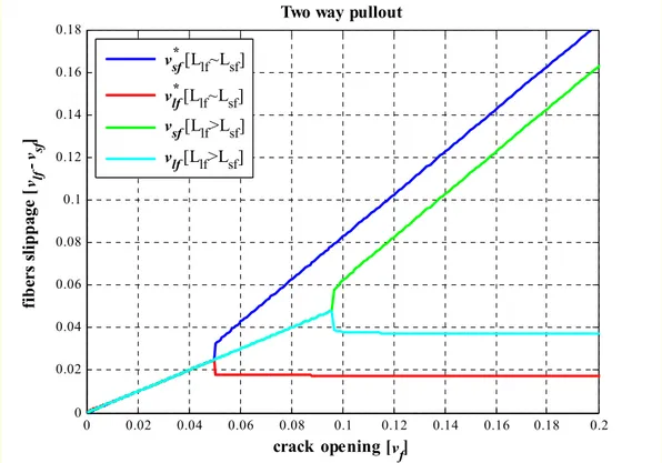
A well-known technique to study fiber-matrix interfacial behavior is single fiber pull-out, Katz. A., Li V.C. (1996). In Fig. 2.1 is shown the typical pull-out curve. Three stages are identified: initial elastic stretching of the fiber free length, followed by debonding stage and at the end the pullout phase.

0 0.05 0.1 0.15 0.2 0.25 0.3 0.35 0.4 0 0.05 0.1 0.15 0.2 0.25 v_f[mm] P f [K N ] v_d Pullout stage Debonding stage Elastic stage

Figure 2.1: Single pullout curve of steel fiber.

The fiber in pullout first is subject to debonding before the pulling out phase takes place. Basically, this can be described as a crack propagation from the surrounding matrix crack to the embedded end. This stage lasts until there is the load drop, that represents the transition to the pull-out stage, when we are left just with frictional bond that can actually increase, whereas the chemical bond, that is present during this first stage, is lost. Stress analysis and energy balance process are used to model the debonding and the pullout of a single fiber. The following are the main assumptions of this model by Z. Lin, T. Kanda and V.C. Li (1999):

a) Fibers are high aspect ratios (>100), so that the final effect on the total debonding load is negligible;

b) During the debonding stage, the slip-dependent effect is negligible since relative slippage between the fiber and the matrix in the debonded portion is small. Hence, the frictional stress within the debonding zone remains at a constant τ₀;

c) Poisson’s effect is negligible. For flexible fiber-cement systems, Poisson’s effect is usually diminished due to inevitable slight misalignment and surface roughness of the fiber;

d) Elastic stretch of the fiber after complete debonding is negligible, compared with slip magnitude.

The relation between the load P and the displacement _f w is written. This is divided in two different equations, matched with the different stages present in the single fiber behavior. At each stage, the fiber extending across the matrix microcrack is always in equilibrium. It is possible to say that the force exerted on the short embedment side and the long embedment side are equal:

( )

sf lf

( )

lf sf

f P v P v

P = =

According to the previous statement, it is also true to declare that in absence of the different effects, the crack opening can be written as:

lf sf f v v

w = +

this is the case when the crack opening is done only by the fibers-matrix slippage. The crack opening, implemented into the code, is composed by three different contributions, given that the model allows to study 3d problems:

[

2 2 2

]

12 Lf Mf Nf f w w w w = + +

In this way, is identified the vector identifying the crack opening created only by the fibers slippage. This crack opening vector is the result by sum of the slippages values, later when the other effects will appear there will be a new crack opening vector, called '

f

w . This will be different than w for direction and modulus. _f

Considering a crack crossed by straight fiber (Fig. 2.2), characterized by the embedment lengths L and _sf L . If one neglects the fiber bending stiffness and the _lf

elastic deformation of the crack-bridging segment, the length of such a segment (distance between points A and B in Fig. 2.2) can be computed as:

f f f

f w s n w' _{= +}2

where '

f

w is the crack opening vector and s the reduction of embedment lengths _f

due to micro-spalling.

a)

φ

_f

’

w

_Nf

w

_Tf

w

_f

L

_sf

L

_lf

s

_f

w

_f

’

_n

_f

A

B

Figure 2.2: Schematic of inclined bridging with matrix spalling.

In additional, the fiber force con be assumed to be coaxial with the crack-bridging segment and expressed as:

' f f f P n P = where: ' ' ' f f f w w n = and ' '2 '2 '2 Lf Mf Nf f w w w w = + + .

The Fig. 2.3 shows the best situation possible, characterized by fiber orthogonal to the crack plane. In this particular configuration the spalling and the snubbing, that will be later explained, are not present.

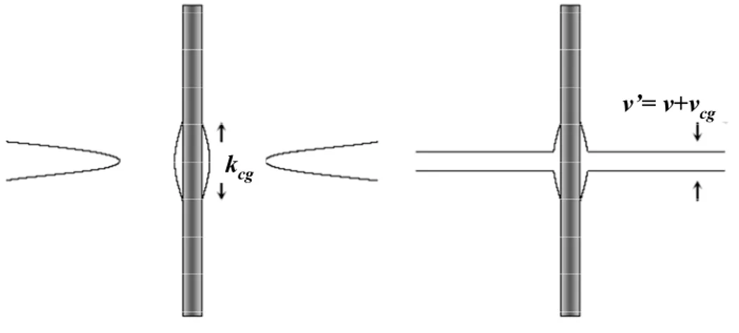
In the next section, will be explained how the crack opening vector changes according to the other effect that the fibers issue shows. The new effect that will be considered is Cook-Gordon effect. According to the change just show before, will be explained also the micro-spalling.

The different stages for a single fiber will be described using different relations that permit to find the link between P_f − and also v σ −v. In this first step, the relation between force and crack opening will be analyzed, assuming that the pullout force is always applied orthogonal to the crack plane. Later on, the same analysis will be performed but looking at most common cases.

In the second step, the strength relations will be introduced. In this way the constitutive law is done.

P , v

L

b)

)

Figure 2.3: Fiber pullout with force applied orthogonal to the crack plane.

Following the detailed derivation by the Z. Lin, T. Kanda and V.C. Li (1999), the equation for the debonding stage can be written as:

( )

(

)

d f f d f fd _v G E d _{v v} E v P = + + 0≤ ≤ 2 2 1 2 3 3 0 2_{τ η π} π

where v is the crack opening that corresponds to the displacement at which full-_d

debonding is completed, and it is expressed as:

(

)

(

)

f f d f f d d E L G d E L v =2τ 1+η + 8 1+η 2 2 0

The elements that appear here are: η=V_fE_f V_mE_m, this is a parameter expressing the ratio of the effective (accounting for the volume fraction) fiber stiffness to effective matrix stiffness, frictional stress τ₀and debonding fracture energy G _d

(also referred to as chemical bond). When the debonding phase is finished, it is possible to see a sudden drop due to unstable extension of the tunnel crack. Subsequently, the fiber is held back into the matrix only by frictional bonding.

The magnitude of the drop can be used to calibrate the chemical bond G . During _d

the debonding and pullout stage, the fiber may rupture if the load P exceeds the

fiber tensile strength. According to this effect, the study is developed under the assumption that the fiber rupture never happen.

The relation that describe the force in the pullout stage is:

( )

(

) (

L v v

)

v v L d v v d v P _{d d} f d f ⎟⎟ − + ≤ ≤ ⎠ ⎞ ⎜ ⎜ ⎝ ⎛ ₋ + =π τ₀ 1 β

The different elements present in this equation, are shown in Fig. 2.4. It is also possible to write the equation for the debonding stage in terms of the debonding length. In this case the debonding load P can be also expressed as:

( )

2 3 2 0 d f f f L G E d d L P =π τ + π

at the full debonding L= . The maximum debonding load is given by: L_e

2 3 2 f f d b a P G E d P = + π

where P_b =πd_fτ₀L_e is the initial friction pullout load. This equation allows calibrating the chemical bond strength G and the frictional bond strength _d τ₀, from the maximum debonding strength load P and the initial frictional pullout _a

load P . The slip-hardening coefficient _b β, is obtained from the relation that is used for the pullout stage.

P , v

L

(v – v

_d

)