Scuola di Ingegneria ed Architettura
Corso di Laurea Magistrale in Ingegneria e Scienze Informatiche
ENGINEERING BEHAVIOURAL
DIFFERENTIATION IN ROBOTS
CONTROLLED BY BOOLEAN NETWORKS
Tesi in
SISTEMI INTELLIGENTI ROBOTICI
Relatore
Prof. ANDREA ROLI
Co-relatore
Dott. MICHELE BRACCINI
Presentata da
ALESSANDRO CEVOLI
Automatic Design
Behaviour Differentiation
Boolean Networks
Robotic Agents
Stochastic Descent Search
Introduction ix
1 Background and State of the Art 1
1.1 Gene Regulatory Networks and Boolean Networks . . . 1
1.2 Applying the Synthetic Biology and GRN Models to the Robotic Field . . . 3
1.3 Responses of Boolean Networks to Noise . . . 7
2 Methodologies 11 2.1 The Adopted BN Model . . . 12
2.2 Goals and the Biological Idea . . . 13
2.3 From Attractors to Behaviours . . . 15
2.4 Automatic Design of a Selective-BN: Achieving controlled re-Differentiation . . . 17
2.4.1 Constraints . . . 17
2.4.2 Network Design . . . 19
2.5 Automatic Design of a Behavioural-BN . . . 21
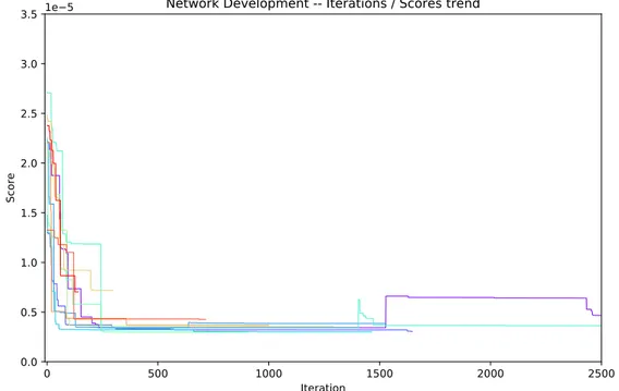
2.5.1 Network Development . . . 21
2.5.2 Design Methodology . . . 24
2.5.3 Testing Methodology . . . 30
2.6 Assembling the Robot Controller . . . 32
2.6.1 Connecting the Networks . . . 32
2.6.2 Testing Methodology . . . 33
3 Results 41 3.1 Experiments Set-Up . . . 41
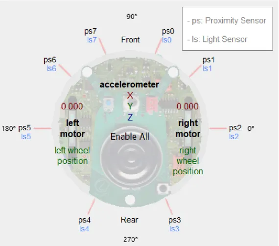
3.1.1 Agent Embodiment . . . 41
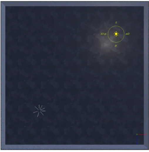
3.1.2 Deployment Environment . . . 45
3.2 Experiments and Results . . . 46
3.2.1 Selective Boolean Network . . . 47
3.2.2 Behavioural Boolean Network . . . 50
3.2.3 Selective Boolean Network Controller . . . 59
Conclusions and Future Work 65
Appendices 69
A Selective Boolean Network Constraints 71
B Boolean Network Controller: Phototaxis 79
C Boolean Network Controller: Anti-Phototaxis 95
D Selective Boolean Network Controller 113
The automatic design of robot control software is an important subject in current robotics; it aims to overcome the characteristics of classical human design, which might result limited and biased, in those cases where the robot task or the environment (in which the agent is situated) can not be formally specified or defined in advance or when the designer wants to explore new solutions. Indeed, automatically exploring the space of possible solutions and pin-point good ones through a series of constraints or performance require-ments that the agent needs to satisfies, like an evolutionary algorithm may do, opens different possibilities to the design of the robotic agent controller, morphology and embodiment that we human would have never thought of. Moreover, such approaches are able to bring forth many necessary properties for agents, like greater degrees of autonomy, robustness and adaptiveness, in a more natural and far flexible way, whether they are on-line or off-line design procedures. Also, automatic design makes it possible to explore and exploit new kinds of control software, mainly those inspired by biological models.
For example, biological cellular systems offer an example of robust, adap-tive and dynamic models where the tight link between artificial intelligence and dynamical system can be exploited. Boolean networks are a gene regu-latory network model introduced by Kauffman [1] which are quite compelling from an engineering point-of-view, due to their rich and complex behavioural expressiveness despite the compactness of the model. Moreover, Boolean net-works are able to reproduce many cellular systems properties and dynamics [2] like: different degrees of differentiation, stochastic and deterministic differ-entiation, limited reversibility, induced pluri-potency and induced change of cell type. Also, it has been shown that behaviours of Boolean network-based robots can be decomposed into smaller elementary behavioural blocks [3], each represented by attractors in the state-space of the dynamic system, connected by trajectories, and controlled by specific inputs.
The main goal of this thesis is to find an automatic procedure that is able to develop, given an initial Boolean network, a robot controller capable of differentiating between two or potentially more behaviours, after certain environmental signals are perceived by the agent sensors. Obviously, the more
variegated the external stimuli are, the more behaviours are more likely to be associated. Moreover, as hinted and exploited in some existing works [4, 5, 2], we assume that the environment is initially permeated by some kind of noise that does not allow the robotic agent to stabilize on a single behaviour but instead equally display all of them.
The major change from other works found in literature, like those by Roli et al. [6, 7], is that, once the agent has adapted for a certain environment, it should be able to go back to its previous pluri-potent state or manifest another behaviour as the environmental conditions change. That is, it should be able to re-differentiate itself as the environment changes.
In Chapter 1 we will initially provide the background and then discuss the state of the art from which this thesis stems.
In Chapter 2 we will talk about the strategies and methodologies adopted to tackle our problem of designing a robot controller based on Boolean net-works and capable of re-differentiating. Then move on, describing how network performance is measured in order to validate the effectiveness of the devised design algorithms.
Finally, in Chapter 3 we will describe the various experiments and envi-ronment set-ups, the adopted agent embodiment and, finally, results on each network design, development and test.
Background and State of the
Art
In this chapter we will introduce the main works that have mainly con-tributed to this thesis, either from a theoretical and methodological or tech-nological perspective. The aim is both to provide the background for the subsequent chapters, and to summarise the state of the art of the main topics covered in this thesis.
1.1
Gene Regulatory Networks and Boolean
Networks
Gene regulatory networks, GRNs in short, are synthetic biology models that have been shown to reproduce most of the dynamics and interactions among genes (Gene Expression) in a cellular system. Among all the dynamics, they are able reproduce the Cell Differentiation and Morphogenesis processes:
1. Cell Differentiation is the biological process where different genes ac-tivation patterns enable cells to undergo differentiation from a pluri-potent/toti-potent/multi-potent state to a more finalized and mature state by following a path along the linage tree.
2. Morphogenesis is the biological process where the different genes acti-vation patterns enable an organism to develop from a more primitive shape to a more functional and adapted one. Instead of differentiating its functional properties and behaviours, the target of the process is the embodiment of the organism, its shape, sensory organs and ”actuators”. Boolean networks are a gene regulatory network model introduced by Kauff-man [1] which are quite compelling from an engineering point-of-view, due to
their rich and complex behavioural expressiveness despite the compactness of the model.
A Boolean network, BN in short, is a discrete-state and discrete-time dy-namical system, represented as an un-weighted and oriented graph where each
node is defined by a binary state xi ∈ {0, 1} and is associated to a Boolean
function fi. Each node represent the expression (1) or suppression (0) of the
i-th gene. The state of the network at a certain instant t is defined as an
ordered vector S(t) = [x1(t), ...xn(t)], where xi(t) is the state of node i at
instant t. The state of each node is updated deterministically or stochasti-cally, synchronously or asynchronously, at each time-step by the output of the
Boolean function xi = fi(xie1(t), ..., xieK(t)), where xie1, ..., xieK are the states of
neighbour nodes e1, ..., eK to node xi. The parameter K defines the number of
incoming edge to each node and can be different for each one of them.
A randomly generated Boolean network, also called RBN, is a BN where both topology and Boolean functions are randomly generated. Alongside the parameters N ∈ Z and K ∈ Z, defining respectively the number of nodes and the number of neighbors to each node, the generation employs a parameter P ∈ [0.0, 1.0] that biases the output of each truth-table entry of the Boolean
function fi during its generation. The higher P is, the easier is to assign the
output True to an entry of the truth-table.
The state of a cell can be represented as one of the attractors in the state-space of the dynamic system. A transition between cell states (n-potent to more specialized) corresponds therefore to a transition between two attractors.
An attractor is a cyclic sequence or pattern of states1 in the network
state-space that represents a stable state of the dynamic system (e.g.: a cell). Start-ing from any state of a BN, after a number of updates, hence a sequence transient states, the network will reach an attractor of some kind. It’s called trajectory the sequence of transient states followed by attractor states. The set of states that leads to the same attractor is called Basin of Attraction. This means that all the possible gene expression patterns constitute the state-space of the BN and, among them, those in stable equilibrium are attractor states and their gene expression profile determine the observable cell type.
Normally a BN is an isolated system, which means that its state is not influenced by external factors: that is, once an attractor is reached, the tra-jectory will repeat the sequence of states in the attractor forever. But, by applying a certain level of noise that randomly flips the state of some nodes in the network, the trajectory may exit from the attractor and move from one stable state to another through a series of transient states in-between. This behaviour can be associated to tumor-like cells [8].
1.2
Applying the Synthetic Biology and GRN
Models to the Robotic Field
Cellular systems are robust, adaptive and dynamic, therefore the tight link between artificial intelligence and dynamical systems can be exploited. More-over, it has been shown that behaviours of Boolean network-based robots can be decomposed into smaller elementary behavioural blocks [3], each repre-sented by attractors in the state-space of the dynamic system, connected by trajectories, and controlled by specific inputs like chemical signals.
The survey [9] by Braccini reviews different methods in synthesizing robotic agents for different GRN-based models. The survey explores three main ap-proaches: those which evolve or generate only the agent controller, those which evolve only the robot morphology, hence the embodiment, and those that at-tempt to achieve both by co-evolving agent embodiment and brain.
In the former, the prominent examples reported are:
• Eggenberger’s Artificial Evolutionary System (AES) [10] which aims to control the main developmental process of the agent controller (in the article a neural controller) by exploiting biological processes like Cell Differentiation, Division and Adhesion, and concepts as Regulatory Units and Transcription Factors, Cell Adhesion Molecules and Cell Receptors. Everything in the model is encoded by an artificial genome composed of Regulatory Units and Control Genes, where the first activate or inhibit the seconds, while the latter modulate the developmental processes by producing substances regulating the activation of the aforementioned biological mechanisms.
• Another model, based on the biological principle of the proteins synthe-sis regulation [11, 12], develops an artificial neural network to control a robotic agent through a morphogenetical process that evolves the shape of the network. The employed evolutionary algorithm defines both topol-ogy, learning rules and weights of the networks, allowing it to synthesize any kind of network.
• The latest mentioned and explored approach is the one presented by
Roli et al. [6]. In the article an effective automatic (meta2) procedure to
design Boolean networks as robotic agent controllers is presented. The design process of the controller is modeled as a search problem, exploiting meta-heuristics, with the goal of minimizing the error in performing the
2Since it’s not bounded nor restrained to the usage of specific meta-heuristic or search
given tasks of phototaxis and anti-phototaxis. The two tasks are alter-nated by a sharp sound signal that has to trigger the behaviour switch. The automation approach can be described as follow:
1. generator – The network is randomly generated, given the number of nodes N, the node arity K and a bias P which is used to randomly generate the output values of the entries in the truth-table of each Boolean function.
2. evaluator – The network is simulated and then evaluated on the basis of the chosen target requirements (objective function).
3. meta-heuristic – Given the results of the objective function, the meta-heuristic process starts the search. In the specific study the used search algorithm is a simple stochastic descent. The search process may lead to change the internal BN structure by modifying
an entry of a truth table3, if the evaluation output doesn’t satisfy
the minimization targeted value.
The article also propose an encoding for a BN-robot that tightly couple the BN and agent morphology/embodiment:
– The generated BN has synchronous and deterministic update, and is synchronized with the robot.
– For each BN a sub-set of I nodes is chosen as input nodes while another sub-set of O nodes as output nodes.
– The sensor readings are binary encoded and dynamically update the state of the input nodes.
– At each step the network is updated with the sensor readings, then it consequently updates its internal state and, finally, the state of the output nodes is applied as control value on the robot actuators. In regard to the morphogenesis of a robot embodiment, the only exam-ple reported is always from Eggenberger [13]. In the article the previous AES model is extended by introducing positional information and pattern formation in the developmental process. This way each cells acquire a positional iden-tity (coordinates) which changes the way the cell interprets the information, accordingly to its genetic constitution.
Finally, among the techniques belonging to the third approach, i.e. the development of both morphology and controller, the most relevant analyzed
is the Artificial Ontogeny [14] which combines ontogenetic development with genetic algorithms in order to evolve a complete agents. In such model, each genome is evolved using a genetic algorithm and treated as a GRNs, each gene produce ”gene products” that either have a direct effect on the phenotype or regulate gene expression. Therefore the whole ontogenetic process enables a translation from a genotype (agent genome) to a phenotype (3-dimensional agent), later evaluated in a virtual environment. Each agent starts its ontoge-netic development as a single structural unit then developed through a geontoge-netic algorithm tinkers on its genetic compound. On the morphological side, each unit has joints to attach itself to other units, carries a copy of the genome and has 6 diffusion sites, which contains any number of diffusing ”gene products” and/or be connected to sensors, actuators or internal neurons. In addition to its embodiment, the genetic process develops the agent neural structure as well: of 24 different ”gene products”, 2 affects which growth units to diffuse into, 17 modulate the growth of the agent neural substrate and 5 genes are devoted to control gene expression.
The aforementioned article from Roli et al. [6] is further inquired in a study on the properties of artificially evolved Boolean networks [7]. In this article a greater focus is given to random Boolean networks in the critical regime with K = 2 and P = 0.5 [15, 16], those on the boundaries between order and chaos. This kind of networks display important properties such as capability of balancing evolvability and robustness and maximizing the average mutual information among nodes. The exploration of this boundary is a main difference from the previous work where the Boolean network controllers were initially generated with K = 3: while still in the critical regime, they are already more on the chaotic side.
The extracted evaluation features proposed in the article are:
• State number and Frequency of state occurrence in sample trajectories – The number of unique states in the collection of trajectories is an index of the state-space occupied by the dynamics. As such, the smaller number of unique states is, the greater the generalization capabilities of the network are, since it denotes trajectories that share a large number of transitions which means that the system was able to generate a compact model of the world.
• Number of fixed point attractors – Is a measure of the generalization capabilities of the system since fixed point attractors represent functional building blocks of the type while <c> do <a>. As such, emergence of such attractors means that the Boolean network was able to extract and exploit regularities inside the environment and classify them.
• An estimate of the statistical complexity of the Boolean network, hence to which extent the system is working in the critical boundary, is given by means of the LMC complexity. The complexity measure is calcu-lated as C(X) = H(X) · D(X), where H(X) is the Shannon entropy, which should be higher for complex networks since they display highly diversified trajectories, and D(X) is the disequilibrium, which should de-crease for complex networks since it estimates to which extent a systems exhibits patterns far from equi-distribution, thus presenting trajectories composed by repetition of few states.
Each feature is calculated by analyzing the BN-robot trajectories in the BN state-space and extracted for each evolutionary step.
The results brought by the article shows that robots, which successfully achieve the target behaviour, are characterized by a decreasing number of unique states as the complexity grows. Also, both entropy and disequilibrium show the expected complementary results for successful networks, leading to a steadily increment of the complexity during the training phase.
A similar and somewhat complementary automatic design approach to [6], concerning the development of Boolean networks with a given set of target properties, but regarding the field of synthetic biology, Cell Differentiation in the specific, is described by Braccini [16, 17]. There, two approaches, both based on stochastic descent, are defined:
• Adaptive Walk – A simple stochastic descent search algorithm where, once a BN is generated, it is iteratively modified by flipping one random entry of the truth-table of one random node in the network, until either the evaluation of the network through an objective function matches the target value or the algorithm reaches the maximum number of iterations. The algorithm allows for sideway moves, that is, flip moves that generate a network with the same objective score to the previous one. This allows the algorithm to explore eventual plateaus in the search space.
• Variable Neighbourhood Search – A more complex search algorithm where the number of flips increases overtime until a better solution than the current one is found. The stop criteria are the same of the Adap-tive Walk. The compelling features of this algorithm is the previously described sideway moves plus the ability to escape from local minima which, in a random search, are very likely to happen.
In the article [3] is inquired the aforementioned direct mapping between attractors and robot behaviours. The main goal of the paper is to exploit the
properties of the attractor landscape in order to control the speed of a robotic agent while performing a simple behaviour like phototaxis. The mapping be-tween the elementary blocks composing the behaviour and the attractors is achieved by means of an adaptive process (a simple stochastic descent). More-over, in such setup, some nodes of the network are directly coupled with the embodiment: some nodes are temporarily switched on by what is perceived by the sensors, while other nodes are chosen to directly control the actuators output.
The BN of the first experiment is characterized by 2 control genes: one assessing the presence of light, while the other is switched on in order to suppress the behaviour as the agent comes too close to the light source, hence stopping the agent in its proximity.
In the same paper is presented another experiment where some nodes, cho-sen as receptors, are permanently clamped to 1 or 0 as a consequence of an external signal. The clamping leads to changes in the transition graph of the BN, cutting off some transitions and therefore the expression of some attrac-tors. Moreover, the action of clamping opens the networks to the expression of conditional attractors: (possibly new) attractors that are conditioned by an external factor (clamping), which impose the agent to specific attractors composed by states with a common pattern.
1.3
Responses of Boolean Networks to Noise
Fretter [5] has explored the probability ρ that a Boolean network (immersed in a noisy environment), once reached an attractor, returns on the same stable state after that h nodes have been perturbed. The experiment hence aims to provide some tools to describe quantitatively the robustness of the network. In the paper, various type of networks are studied: independent nodes, simple loops, collection of single loops and RBNs. For RBNs, different K are used: K = 1 for frozen phase networks, K = 2 for critical networks and K = 3 for chaotic networks. In this cases, the results show that for K = 1 the probability
ρ varies widely, and is easily larger than ρ = N2. On the other hand, chaotic
and critical networks show interesting results: RBNs with K = 2 display lower robustness than those with K = 3; in the first case ρ can be described as
ρ = (aN−13)h, while for chaotic network ρ rapidly decrease for small h and
then sits on a plateau always around ρ = 23.
This difference between critical and chaotic RBNs can be attributed to the difference in the number of attractors between critical (higher) and chaotic (lower). It is therefore easier for RBNs with K = 3 to go back to the same attractor once perturbed since more states will belong to the same basin of
attraction.
In the end, all the result have been achieved by means of randomly gen-erated networks but, generally, the topology of the network has a consistent influence on the on the dynamics of the network and, therefore, on the number of expressed attractors.
For low level of noise (perturbation ∼ 1 node at time), it is possible to draw an attractor graph and the correlated Attractor Transition Matrix, where for
each pair of attractor (ai, aj) is assigned a probability ρ describing how easily,
in presence of noise, the network can move from one stable state to another. An effective metaphor describing the attraction basins, called the ”Epigenic Landscape”, has been provided by Waddington [18]: the network state is like a marble that rolls down the landscape topology until it reaches a local min-ima, that is, an attractor.
A mathematical model, called the Threshold Ergodic Set (TESθ),
reproduc-ing the abstract properties of Cell Differentiation4 has been proposed by Serra
and Villani [2]. In this model the notion of Ergodic Set previously proposed by Ribeiro and Kauffman [4] is extended by means of a threshold θ ∈ [0, 1] that cuts off from the attractor graph those transitions (between attractors) such that ρ < θ. An Ergodic Set is a subset of the all possible attractors that entraps the system for t → ∞. Since there is usually only one of such sets for most Noisy (Random) Boolean network, the proposed model introduce the threshold θ in order to split the attractor graph into smaller (possibly isolated)
TESs, till a single TES is composed by a single attractor. Therefore, a TESθ
is a ES where attractors are directly or indirectly θ reachable.
The similarity with the biological model and TESθis that wandering through
a large number of attractors could be associated to a toti-potent cell while,
as the threshold increases, smaller TESθ appears which corresponds to more
differentiated biological forms. The TES composed by single attractors are, therefore, the fully differentiated cells.
Since different noise levels are usually associated to different level of differ-entiation, the increasing of the threshold θ would correspond to a decreasing level of noise in the biological environment.
4Different degrees of differentiation, stochastic and deterministic differentiation, limited
Conclusions In the end, many have dealt with the problem of automati-cally design robot controller based on synthetic biology models; among them, Boolean networks are interesting due to their simple model, robustness, adap-tiveness and dynamism typical of cellular system, and the ability to reproduce some of the cell properties and dynamics. The usual approach to the design process is to employ meta-heuristic strategies based on stochastic descent and therefore to randomly explore the solution space. The results of the design processes appear promising especially when evolving the sole Boolean func-tion paired to each network node, while keeping intact the network topology. Furthermore, if noise is exploited in the design process, it may open new pos-sibilities to generate networks with certain level of robustness.
In the next chapter we firstly connect together many of the methodologies and information expressed in this Chapter, through the analysis of these vari-ous articles, then improve with novel approaches those which will be employed to achieve the primary goal of this work.
Methodologies
In this chapter we introduce and describe the methods applied and solutions adopted to attain behavioural diversification in robots. We identify as BN-robot any kind of BN-robotic agent equipped with a controller based on one or more Boolean networks, where some node are employed as sensor receptors while others interface with the agent actuators.
The work is divided in two main parts: one involving the automatic design of a Boolean network able to achieve a specific non-trivial task and that could employed as a stand-alone robotic agent controller, similarly to Roli et al. [6]; while, in the other, we move to design a Boolean network that is able to express controlled re-differentiation by satisfying a certain number of constraints. Such BNs will be employed to compose a hierarchical control unit that differentiate into any given number of behaviours.
A bit of terminology Before going on, it would be useful to specify and
clarify some of the terminology that will adopted from now on in this work. The words agent, robotic agent and robot are used interchangeably. It is always implied that the agent is a robot equipped with some kind of Boolean network-based controller.
As previously stated in [3], a direct mapping between network attractors and robot behaviours can be achieved; as such, the words attractor and robot behaviour will be used interchangeably.
When talking about the display or expression of a certain attractor on a given BN, we imply that the network state is updated for some time until an attractor is displayed.
For noise phase and transition phase we mean those time-steps where the BN is affected by perturbations due to the presence of noise or when, due to some changes in the environment, the network move from one attractor to another. These transitions between attractors, called transients, are usually
compound of states that are not part of an attractor per se but uniquely lead to it (when not under noise).
While discussing the simulation of the network, either to evaluate or test it, we refers to the triplet agent initial position, agent initial rotation and <type> source initial position as starting configuration.
2.1
The Adopted BN Model
All Boolean networks in this work are random Boolean networks – RBNs [19, 17] characterized by synchronous and deterministic update sequences, like most of the networks explored in the articles presented in Chapter 1, and described by the following main parameters:
• N ∈ Z – the number of nodes in the network.
• K ∈ Z – the number of neighbours/predecessors of each node. Hence the number of inputs to each associated Boolean function.
• P ∈ [0, 1] – the bias to assign either True or False to an entry of any Boolean function truth-table in the generated RBN.
• Q ∈ [0, 1] – the bias to assign either True or False to a node as initial state when the RBN is generated.
While not explicitly defined in their signature, the model of all the networks also support noisiness – NRBNs [19, 17]. The level of noise in the network is
regulated by means of a parameter ρnoise ∈ [0, 1].
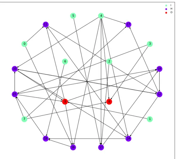
An Open Boolean Network, OBN in short, is a kind of BN which have some nodes assigned as receptors and others as actuators [6]. They are characterized by two more control parameters, named I ∈ Z and O ∈ Z, which define respec-tively the number of input and output nodes in the network. We identify as input nodes those nodes which will be employed to receive feedback from the environment, while output nodes are those adopted to communicate or inter-act with the environment. This is the model on which any Boolean network controller in this work is based upon, therefore all the developed robotic agents that will be developed are indeed BN-Robots.
For simplicity, input and output nodes are chosen sequentially inside each network; that is, if the network has N = 20, I = 8 and O = 2 then nodes ∈ [0, I) are input nodes, while nodes ∈ [I, I + O) are output nodes.
2.2
Goals and the Biological Idea
The main goal of this thesis is to find an automatic evolutionary or search procedure that is able to develop, given an initial Boolean network, a robot con-troller capable of differentiating between two or potentially more behaviours, when certain environmental signals are perceived by the agent sensors. Obvi-ously, the more variegated the external stimuli are, the more behaviours are more likely to be associated. Moreover, as hinted and exploited in previous works [4, 5, 2], we assume that the environment is initially permeated by some kind of noise that does not allow the robot to stabilize on a single behaviour but instead (more or less) equally display all of them.
On a biological level we could describe the robot dynamics as a pluri-potent stem cell that is initially immersed in a solution (environment) characterized by highly mutability and dynamism, such that the cell is not able to find a stable pattern of signals on which develop itself among the chaotic series of stimuli it receives. Then, as the noise subdues and the environment becomes more and more ordered, the cell is able to determine a pattern in the series of
signals1 and develop itself, evolving along a certain branch of its lineage tree.
Until this point the work described mostly follows the tracks already laid down by Roli et al. [6, 7] and correlated works. The breaking change from the previous material that we aim to achieve is: once the agent has adapted for a certain environment, it should be able to go back to its previous pluri-potent state or manifest another behaviour as the environmental conditions change. That is, it should be able to re-differentiate itself as the environment changes.
This dynamics can be associated (to a certain degree) to the behaviour of a cancer cell [8] which, if stressed with enough stimuli, could undergo a re-differentiation process that brings it to a cancer state, which may be seen as a pluri-potent stem-like state. What we want more is for it to even develop to a completely new non-cancer cell.
In order to achieve what expressed above, the work has been mainly cut down into three sub-problem:
1. First, devise an automatic design procedure that generates a single Open Boolean Network satisfying the following constraints:
• The network has only M attractors.
• While perturbed, for each attractors pair (ai, aj), the transition
probability ρij | ai → aj must be greater than a given threshold τij.
• While under the effect of noise the network displays all the attrac-tors, independently from their frequency.
• While unaffected by noise, given a specific input stimuli, the network displays always the same attractor regardless of the initial state. That is, they are able to express re-differentiation: to come back to their pluri-potent state or move to other attractors once the environmental signal change, while expressing all their possible behaviour and displaying a selected number of behaviours, much like a cancer cell would do. This kind of networks usually have no output nodes and a number of input
nodes I such that the possible stimuli to be perceived are 2I.
Such Boolean networks, will be either referred to as Control-BN – CBN or Selective-BN – SBN, interchangeably, in order to distinguish them from other Boolean networks.
2. Then, with another ad-hoc automatic procedure, generate an OBN
achiev-ing a very specific behaviour. Such kind of networks will be called
Behavioural-BN – BBN in order to tell them apart from the networks specified on point 1. They can effectively be adopted as stand-alone robot controllers.
3. Finally, achieve an efficient and flexible mapping methodology between the attractors expressed from the network developed in point 1 and the behaviors expressed by the networks evolved in point 2, that is: mapping an attractor to another whole Boolean network.
We have chosen to do so in order to, from an utilitarian point-of-view, simplify both evolutionary procedures while, on an engineering point-of-view, achieving flexibility and generality of the generated networks: instead of de-veloping a whole network which attractors represents the wanted ad-hoc be-haviours and satisfying the cancer-like constraints, it is far more valuable, especially for testing and study purpose, to have a generic network which presents the said cancer behaviour while its attractors can be whatever and only ontologically associate them with a given behaviour.
The whole structure, composed by a single SBN and M different BBNs, will be referred to as Selective-BN-Controller – SBNC.
2.3
From Attractors to Behaviours
Starting off from the last on the three sub-problems, we will point out the main idea behind the chosen mapping method.
Given a produced Selective-BN, such network will display the given num-ber of M attractors, each of variable length, and its Attractor Transition Matrix
will display, for each element, a transition probability ρij greater than the
spec-ified threshold τij. Being M the number of possible assignable behaviours, then
each state composing one of the M attractors should uniquely lead to a specific behaviour. But, in doing so, which behaviour to choose when the network is not on an attractor? More specifically, since the network has to equally display each behaviour when affected from noise, how to map each behaviour into a network state when this is not part of an attractor?
There are two possible solutions to such dilemma:
• State graph approach – One is to simply assign a behaviour to a known at-tractor and, based on the complete state graph of the developed network, unambiguously map each state in the graph to the behaviour associated to the attractor the graph refers to. While doable, the approach seemed quite expensive computationally and memory wise since the graph size
may not be trivial and its complexity is O(2N).
• ATM approach – As before, simply map each behaviour to a known attrac-tor but, this time, each state composing the attracattrac-tor uniquely leads to the mapped behaviour while, for non-attractor states, randomly choose which behaviour to express by weighting each choice with the transition
probability ρij | ai → aj described in the network Attractor Transition
Matrix. Since non-attractor states will appear only during noise phase or in transients of a trajectory leading to an attractor, this approach works during both noise phases and transition phases, when the network is either regressing to a pluri-potent state or moving from one behaviour to another.
In the end, among the two above described methodologies, the chosen one is the ATM approach since it gives a more concise and simple solution, even if determining a network ATM may be an expensive operation for big Boolean net-works. Also, while both approaches are equivalent when the network is stable on an attractor, the precise mapping between transients states and behaviours given by the state graph approach isn’t needed. Moreover, realistically speak-ing, having transition phases is far more interesting than selectively changing attractors like an if-statement would, since this transition can be interpreted
as the adaptation process of the network to the new environmental conditions. Also, it better outlines the real behaviour of the network if the expressed at-tractors were (sort-of) the behaviours themselves.
Furthermore, in order for the mapping to be more flexible, instead of di-rectly associating attractors to behaviours, each behaviour is uniquely and a priori associated to a possible input stimuli while, during the development phase of the SBN, each attractor is dynamically associated to the input stimuli that induce the network to transit always on that attractor, whichever the initial state of the network may be.
Still, letting behaviours being imposed by transition biases means that there is no certainty on which behaviour will prevail, on the short term, due to the randomness (especially in a noisy environment). Surely enough, in a long term run, the ratio of alternating between behaviours will definitely match that expressed by the ATM. Moreover, a factor to be wary about during behaviour analysis is that, since behaviours can vary greatly in what they do, some of them will surely negatively influence those who comes after. This is true for both aforementioned approaches. To give a proper example: given an agent that has to express both phototaxis and anti-phototaxis, it is possible that either of the two behaviours has more influence on the global conduct than the other, be it due to random fluctuations in the behaviour choice or an
higher average speed of one of the behaviours2. As such, if anti-phototaxis
is expressed first then it leads the agent further away from the light source which will influence negatively the evaluation of phototaxis.
2Since they are designed by an automatic procedure is not a possibility that can be
2.4
Automatic Design of a Selective-BN:
Achieving Controlled re-Differentiation
In this section we’ll move on, describing the approach undertook to tackle the problem of automating the development of the Selective-BN.
A Selective-BN usually has no output nodes but only a number of input nodes that depends on the environmental stimuli that guide its differentiation process. In our scenario the environmental signal is binary, hence a single input node with each stimuli leading to a unique behaviour: 0 → phototaxis or 1 → anti-phototaxis.
2.4.1
Constraints
As previously mentioned, the target Boolean network must satisfy four constraints:
1. The network expresses only M attractors, of any length, when situated in a noisy environment.
2. For each attractor pair (ai, aj), the transition probability ρij for moving
from ai → aj, while the network is perturbed, must be greater than a
given threshold τij.
3. While under the effect of noise, the network displays all the attractors, independently from their frequency.
4. While unaffected by noise, given a specific input stimuli s, the network
expresses always the same attractor ai regardless of the initial state, after
φ update steps.
Note that, even if the number of stimuli is 2I, it doesn’t mean that the
number of behaviours to be displayed must amount to that: k different stimuli may lead to the same attraction states, what matters is that all the attractors (M) are mapped into at least one stimuli.
What we want is for the network to be robust enough to always return to the same attractor [5] but only for a certain set of stimuli localized on a defined portion of it topology (the input nodes).
Also, the mapped stimuli will define to which behaviour the attractors are associated since the association stimuli-behaviour is defined a priori.
The constraints are each characterized by some control parameters: 1. M, the number of attractors the network should display under noise.
2. τij, ∀ i, j ∈ A 3, specifies a lower-bound for transition probability ρij
that must be met for each entry of the network ATM.
3. (a) i, the number of iteration for which the BN should be updated in
order for all the attractors to surely appear at least once.
(b) ρnoise, the probability to apply once for iteration a perturbation on
a random node. The perturbation consists in a flip of the state value in the chosen node, as similarly done in previous works [6, 5, 19]. The choice of the noise bias ρ is some what critical: high values of noise increase the difficulty in satisfying the constraint #3, which depends also on the length of the attractors of the network. If the length is short, like between [1, 3] states, then it is easier to display them for higher level of noise since it’s less probable for short sequence of states to be broken. Indeed, if noise is sure to take effect (ρ = 1.0), then it will be impossible to display any attractor with length greater than 1 and, even for such length, everything depends on the noise, which has to place the network in a state inside the basin of attraction of that attractor. Lower value of the bias make it possible to display longer attractor but, on the other hand, it make easier for the network to get trapped into an attractor for long times, letting it unable to express other attractors.
4. φ expresses for how many steps the input stimuli should be imposed on the input nodes of the Boolean network. This also sets a higher-bound to the number of steps the network has in order to adapt to new environmental conditions. Biologically this can be associated to a deafening of the cell to the stimuli.
Notably, the last of the constraints is the hardest to achieve since from [5] we know that networks with higher K tend to be more robust to noise with a probability to return on the original attractor (once perturbed) of
approxi-mately 23. This means that for more chaotic networks is far more difficult to
achieve constraint #4 than for those in the critical boundary.
Moreover, the evaluation of constraint #4 is quite expensive since it
re-quires to test each possible starting state (2N) to be properly achieved. In this
work the problem has been simply brute-forced with some multi-processing since we where working on small enough networks.
While constraint #2 is computationally very easy to achieve per se, it
becomes computationally harder as τij → |A|1 : more and more networks must
be generated before one met this requirement since each ρij → |A|1 for increasing
τij.
2.4.2
Network Design
Since the problem requires the satisfaction of a number of constraints, it can be modeled as a rather simple Constraint Satisfaction Problem – CSP. The employed solution to tackle with this kind of problem is a Generate-And-Test algorithm, given that we will explore small networks with N ≤ 10, where the generation phase always produce a new Open Boolean Network at each unsuccessful iteration while the test phase verifies that all the above specified constraints are satisfied.
In our case study, the randomly generated OBN has the following properties: each of its input nodes has at least one outgoing edge and any node is devoid of self-loops.
Algorithm
A pseudo-Python code regarding the meta Generate-And-Test algorithm and the constraints is provided below.
def GenNTest(max_iters, generator, tester, evaluator):
it, score, sol = 0, None, None
while it < max_iters and not score:
sol = generator()
score = evaluator(tester(sol)) it += 1
return sol if score else None
def test_attractors_number(bn, M): # Constraint n.1
return len(bn.atm) == M
def test_attractors_transitions(bn, taus): # Constraint n.2
def test_space_homogeneity(bn, i, rho): # Constraint n.3
states = [bn.noisy_update(rho) for _ in range(i)]
return len(search_attractors(bn.atm, states)) == len(bn.atm)
def test_attraction_basins(bn, phi): # Constraint n.4
attrs, params = dict(), product(states, inputs) # 2^N * 2^I
for s, i in params:
bs, as = test_state_attraction(bn, s, i, phi)
if len(as) > 1 or bs in attrs and attrs[bs] != as[0]:
return False
attrs[bs] = as[0]
return attrs if len(set(attrs.values())) == len(bn.atm) else False
Description
In test attractors transitions, the parameter i employed in our case study is dynamically set to:
i = 4 ·max|A|
k=0(|ak|) · N
2
where N is the number of nodes in the network and max returns the cardi-nality of the longest attractor of the network. The multiplicative factor 4 is used to slightly increase the number of iterations.
The test state attraction function, once assigned the new state to the network and applied the related input values on each the input node, updates the networks and scans its trajectory until an attractor is found. It then returns the given input and a list of found attractors. The list of attractors should contains only one element since we look for a Boolean network that for a given input, whatever the internal state may be, always moves into the same attraction sequence after at least φ steps.
The if-statement condition on constraint #4 checks whether, for the same input, different attractors have been found or not; that is, if the network moves to different attractors from two different starting states for equal input values.
2.5
Automatic Design of a Behavioural-BN
At last, we will describe the chosen solution to resolve the automatic de-sign of the behaviour-achieving network, which completes the robot controller as a whole. The design process is mainly composed of two phases: (1) a development phase, where the network is generated and improved through a meta-heuristic algorithm, and (2) a test phase, where the developed net-works are further studied to determine their performances.
In the next subsections we will firstly describes the proposed parametric Variable Neighbourhood Search algorithm, pVNS in short, then move on, outlining how and which data are gathered in order to describe the proposed objective function and, finally, the employed evaluation methodology for both development and testing.
2.5.1
Network Development
In previously described works [6, 16], the problem of automatically design a Boolean network with certain given characteristics is modeled as a simple search problem and resolved by exploiting a meta-heuristic search algorithm. Both works indeed outline an approach quite similar to resolve the design problem:
• In [16], as mentioned in Chapter 1, is proposed an interesting meta-heuristic algorithm: a version of Variable Neighbourhood Search – VNS, hence based on stochastic descent, that incrementally improves a given solution until a target condition is met.
• In [6] an evaluator procedure is adopted to produce an objective func-tion score based on a set of target requirements; such value is in turn given as input to the meta-heuristic algorithm that consequently mod-ifies the network through a search procedure (for example a stochas-tic search like above). While the given description is rather generic, it matches both the previously described Generate-and-Test and the above VNS algorithms: (A) both adopt an evaluator function, the for-mer to test the target constraints are satisfied while the latter to assign a score to a new solution. (B) Both try to improve the solution through some kind meta-heuristic strategy: the former generates a completely new solution on each iteration while the latter incrementally modifies a given initial solution. In the end, both methods adopt a stochastic descent search but applied on different levels of abstraction.
In this work the proposed approach arises by improving the VNS algorithm in order to adapt the solution to effectively tackle our problem.
The Generate-and-Test algorithm, adopted in Section 2.4, hasn’t been considered since the problem at hand doesn’t involve the satisfaction of some constraints, hence can’t be modeled as a CSP, but rather concerns the evolu-tion of an already existing soluevolu-tion to meet a certain level of performance in achieving a task. Moreover, even if this problem could be modeled as a CSP and resolved through a Generate-and-Test algorithm, it would be rather in-efficient since on each iteration a new random network would be generated, losing all the good properties of a possibly good-but-not-perfect previous so-lution. On the other hand, the contrary could be a rather good alternative: tackling the CSP problem described in Section 2.4 with an VNS algorithm would probably result more efficient for larger networks since the solution would be improved iteratively rather than be quickly discarded.
Since the evolutionary procedure is done offline, each evaluation of the net-work will require a simulation on a robotic agent. As such, on each simulation some information will be gathered in order to evaluate the behaviour of the agent and produce the objective function score.
Algorithm
def ParametricVariableNeighbourhoodSearch(
sol, target, evaluator, comparator, scrambler, tidier,
max_iters, min_flips, max_flips, max_stalls, max_stagnation):
score = evaluator(sol)
it, flips, n_flips, n_stalls, stagnation = # Init variables
while all(it < max_iters, not stop, not comparator(score, target)):
sol, flips = scrambler(sol, n_flips, flips) new_score = evaluator(sol)
if comparator(new_score, score):
score = new_score
stagnation, n_stalls, n_flips = # Resets values
else:
sol = tidier(sol, flips)
stagnation, n_stalls = # Increase both by 1
if n_stalls >= max_stalls:
n_stalls, n_flips = # Reset stalls and increase flips by 1
stop = # Checks if max stagnation or flips are exceeded
it += 1
Description
Highlighting the differences between the proposed parametric-Variable Neighbourhood Search algorithm and the original from Braccini [16] we can see that:
• The output of the evaluation function, previously defined as distance, is here renamed score. Its type depends on the implementation of the given evaluator procedure.
• The counter noImprovements, that would register the number of itera-tion without improvements before increasing the number of flips, is here renamed n stalls.
• The parameter max flips has been added in order to support different level of scrambling, from more coarse to finer grain.
• Another counter has been added, stagnation, that stops the algorithm when there have been a number of iterations without any improvement equal or greater to max stagnation, regardless of max flips. This also introduce a panic button that would stops development of networks that took too long for too little.
Furthermore, the proposed solution is indeed parametric:
• evaluator – Implements the strategy that tests and assigns a score to a solution. It takes the place of the ComputeDistance function and takes only the solution as parameter. This has been done to maintain the algorithm ”compact” and more generic, but eventually more parameters can be given from outside by exploiting high-order functions.
• comparator – Implements the strategy that compares the found score with the given target value. Takes the place of the comparison between found distance and target distance, allowing more complex comparisons to be made. Depending on its implementation, sideway moves may be either allowed or not.
• scrambler – Together with comparator it represents and implements the meta-heuristic algorithm that adapt the network based on the score returned by the evaluator. It takes place of both the operations of GenerateFlips and ModifyNetwork, that is, it should do both: scramble the network until its changed. Like in [16], the function signature takes as input the previously applied flips in order to avoid repeating them between successive iterations.
• tidier – Takes place of ModifyNetwork when is used to restore the solution to a previous version. That is, if the comparator procedure has returned a score worse than the current one.
Before defining how the four parametric functions have been effectively realized, it is better to first define which data are collected from each simulation of the Behavioural-BN.
2.5.2
Design Methodology
Initial Solution
In our case study, similarly to networks developed by the previous auto-matic procedure, the initial solution is a random Open Boolean Network such that:
• Each input node has at least one outgoing edge and none incoming. • Each output node hasn’t edges outgoing to or incoming from other output
nodes.
• No self-loops are allowed. Target Behaviours
As already said, the target behaviours that the agents have to achieve are phototaxis or anti-phototaxis. We’ll now describe what we expect from an agent achieving these behaviours:
1. An agent achieving phototaxis should move from any point of the envi-ronment, be it near or far away, to the closest possible proximity to the light source.
2. An agent achieving anti-phototaxis should, instead, move from any point of the environment, be it near or far away, to the furthest possible distance from the light source.
Robot Simulation
As previously mentioned, the evaluation of the network requires its simula-tion on a robotic agent for each step of the algorithm. Therefore, the objective function will base its evaluation on the data collected during such simulation. The collected data obviously varies depending on the task to be achieved by the agent and its embodiment; getting this work as example, since the agents
have to learn phototaxis or anti-phototaxis, the data from each equipped light sensor are obviously required.
Some useful data to be collected are therefore:
• <type> sensors data – In our scenario, light sensors data.
• source position – useful to keep track of its position, especially if it’s in motion but that is not our case.
• agent position – useful for multiple reasons, like plotting agent path in the environment or, if paired with the source position, to be used as corroborating factor for the evaluation score during either training or testing.
• network state – useful to study dynamical properties of the network and its attractors as in [7].
• step number – necessary to maintain order among the collected data and, knowing the simulation basic time-step, tell at which time of the simulation the data have been gathered.
Not all the data here described are necessary for the evaluation of the network behaviour but are indeed orthogonally useful for testing or later in-vestigations. In our case study the only data used during network automatic development are the values perceived from the light sensors since we wanted for the agent to improve based on its own perceptions (situatedness).
The objective function Since in our work the agents have to achieve
phototaxis or anti-phototaxis, there is need of a feedback that lets agent understand whether or not is doing its job right. The proposed objective function assigns a score s to a single simulation run by aggregating all the perceived irradiance measurement (in that run) as follow:
s = hmax(stepX s) i=0 |SIR| max j=0(Iij) i−1
where |SIR| is the number of light sensors, while Iij is the irradiance value
perceived at step i by sensors j. Everything is elevated to -1 in order to align
irradiance and distance from the source, since irradiance ∝ d12; this way the
Note that optimal scores greatly depend on (A) how much time is given to
the agent to perform its task and (B) the intensity of the light source4: more
time means possibly higher scores with equal growth trends, but greater in-tensity leads to a faster increase of the score in equal time lapses, especially for agent far away from the light. Moreover, remember that for anti-phototaxis its score will continue to decrease as long as it’s exposed to the light, since the max of the light sensor readings will be non-zero. The pace at which their score decreases depends on the distance at which the agent is and how fast it gets away. Therefore, on anti-phototaxis will be rewarded those networks that get far away from the source as fast as possible, which will reflect in an higher score.
The proposed score model must be indeed minimized for phototaxis while maximized for anti-phototaxis.
Another possible approach would have been to also sum all the perceived sensors values on one step:
s = hmax(stepX s) i=0 |SIR| X j=0 Iij i−1
Such approach has been discarded since the local contribution from the sin-gle sensor would get lost. For example, given two agent learning phototaxis: one near the light but with few sensor oriented in its direction while the other more distant but with more sensors oriented to the source. There may be a situation where each single sensors of the nearer agent has single measurement values greater than those on the further agent but the global contribution of those on the latter are greater than those on the former. This would lead to reward more those agents that get more sensors exposed to the light source by maximizing their global contribution instead of simply going in the direction where the stronger perceptions are sensed.
Moreover, given an environment characterized by n light sources, with the proposed score model the agent is more likely to go towards the source with the stronger intensity or that seems to irradiate greater energy, while the other method would probably lead the agent to go in the (not precisely) middle of the n sources.
One more alternative approach would have been using the error function provided by [6] and using only its phototaxis or anti-phototaxis contribu-tion:
E = α(1 − Ptc i=1si tc ) + (1 − α)(1 − PT i=tcsi T − tc )
This model hasn’t been chosen in order to provide a different evaluation that would use only data local to the agent, that is, given by its own point-of-view on the world.
Scrambling, Tidying, Evaluation and Comparison
In our scenario the four parametric functions, which outline the automatic development algorithm overall behaviour, have been designed as follow:
• scrambler – This function, as previously stated, encapsulate both flips generation and network modification. Both generation and modification are rather trivial since they behave the same as in the work by Braccini [17]: the former produce a number of flips equal to the n flips variable, while the latter apply these flips on the network.
A flip is a pair composed of a node label and a truth-table entry and is applied on the network by negating the output value of the specified table entry. Moreover, in order to improve the stochastic search strategy, the
input and terminal nodes5 of the network are excluded from any flipping.
In this case study, like in previous works [6, 16], we will not explore the development of the network topology but only of its internal structure. • tidier – Like above, this function behave the same way as in the work
by Braccini [17]: given a set of last flipped table entries, the function applies the flip on each specified entry. Since each entry is a binary value, the procedure returns the network to its previous incarnation by negating the actual entry value.
• evaluator – Like already said, an evaluation of the Behavioural-BN requires its simulation. The problem is that a single simulation is only
able to test a single possible starting configuration of the agent6. That
is, one simulation is insufficient to effectively check whether or not the network is able to successfully complete the target task. To this extent the employed approach has been, for each evaluation, to execute T simu-lations, each associated to a different starting configuration. The number
5Nodes that have no outgoing edges and that are not output nodes.
6We identify as starting configuration a triplet composed of the agent initial position and
of simulations T shouldn’t be exhaustive but rather enough to assert that the network behaves adequately in most interesting configurations; the rest is left to the generalization capabilities of the network.
Furthermore, in order to minimize unnecessary score fluctuations due to spawning the agent too close or too far away from the source, it has been chosen that all the starting configurations must be characterized by the equal agent initial positions, same light source initial positions but variable agent rotations. The initial distance between the agent and the source must not be small, that is, it should be wide enough to fully employ the given simulation time to reach the target. Hence, during training are rewarded more all those networks that successfully reach the light source.
Each simulation scores s is then aggregated with the others to produce a global score vector (m, d), which components are mean and standard deviation: (m, d) = PT t=0st T , s PT t=0(st− s)2 T
In order to explain why such statistics have been chosen, let us first list the possible examined alternatives. For simplicity lets consider only the the case of phototaxis:
– Get the worst value (maximum) among the simulation scores: given global score s, if a successive evaluation has overall better scoring but same worst case then it would be accepted as new solution for a sideway move but, at the same time, if a successive solution has
overall worse scoring but better worst case7then that solution would
also be chosen. This lead to an oscillating trend in the function overall scores that nullifies previously done work.
– Get the best value (minimum) among the simulation scores: sim-ilarly to the above explanation, the overall contribution is never taken in consideration thus leading to unbalanced networks where are rewarded those lucky enough to get a favorable starting config-uration.
– Get the median value among the simulation scores: like for the worst case approach, if solution with same median but overall worse
scoring is found, either higher Q1 or Q3, for the effect of sideway moves that solution would be chosen.
– The same would happen when using only the mean as global score, even if vaguely attenuated since the mean already gives an idea of the overall contribution of each score.
The usage of standard deviation samples only those sideway moves with overall better scoring, even when the mean scores are equal. That is, given solutions with equal mean scores, the comparator will look for those with single scores nearer to one another. Instead, for different mean scores, it will always look to the smaller one, independently from their standard deviation. One downside of this approach is a possible over-training of the network: this can be avoided by imposing an adequate target score that is neither too small nor too big.
Note that for anti-phototaxis the above reasoning still stands, obvi-ously remembering that each scores should be maximized instead. • comparator – As anticipated while describing evaluator, the evaluation
score to be compared against the target score is a vector (m, d):
compare((m, d)i, (m, d)∗) =
(
mi < m∗ if mi 6= m∗
di < d∗ else
In both cases sideway moves have been kept but handled in a different manner than in the original idea: instead of allowing all the solutions with scores equal to the current one, the solution are sampled through the standard deviation in order to get only those that effectively move towards an improvement of the solution. An interesting note, observed during the experiments, is that even if the score of new found solutions visibly fluctuates with each minimal changes in the network internal structure, the sub-space of new solution still appear plateau-ish since equivalent solutions are far from being rare. Therefore, sideway moves still work as intended in the original work of [16].
2.5.3
Testing Methodology
The testing of the Behavioural-BN exploits most of the methodologies previously described and is divided into two phases: data collection and data analysis. The main scope of the tests is to assert whether the development procedure is able to create capable networks most of the time.
Data Collection
The primary concerns in this phase is to execute Z test instances, each con-stituted by T simulations and paired to a random starting configuration. The collected simulation data (see Section 2.5.2) are aggregated into the following data:
• agent score – Is the main descriptor of the agent overall behaviour as described in Section 2.5.2.
• agent initial y-axis rotation and agent initial distance – They give an approximate estimate of the difficulty of applying the behaviour to the current task. For example: achieving phototaxis from near the light and oriented in its direction is far more easier than achieving the task from very far away with the agent front opposed to the source. The initial distance is given by the euclidean 3D-distance between the agent position and the light source position, both at the simulation step 0.
• agent final distance – Necessary to corroborate the agent score: dur-ing phototaxis, the smaller the score, the smaller the final distance; in anti-phototaxis, the greater the score, the greater the final distance. The final distance is given by the euclidean 3D-distance between the agent position and the source position, both at the final step of simula-tion.
Along the agent score, in order be able to better reward worthy networks, another scoring model ws has been employed. It is however obtained by nor-malizing the agent score by the ratio between the agent final distance and the agent initial distance:
wszt = szt·
fdistzt
idistzt
The idea is to reward even those network that starts from disadvanta-geous distances, regardless of the agent orientation, since they may be cor-rectly achieving the target behaviour without being able to effectively reach the proximity of the light source or escape far away due to the limited time.
For example during phototaxis, since the score should be minimized, the
ratiofdistik
idistik → 0 as the agent correctly execute the behaviour from far away and
moves closer to the source, hence further decreasing the score. This is especially significant for those networks that start moving from far away, while it remains quite unchanged for those who start already near or just slightly move from
their initial position since fdistik
idistik → 1. While executing anti-phototaxis
the idea is similar but, since the score has to be maximized, the score will grow larger as the agent starts nearer from the source and gets further away: fdistik
idistik → ∞. For those networks that instead already start from afar or remain
suspended under the light, the score remain unchanged since fdistik
idistik → 1.
This scoring approach differs greatly from the one used throughout devel-opment phase since, there, only knowledge internal to the agent could be used. Moreover, during development, all agents and light source were placed always at the same coordinates, while, in testing, the agent initial position can be whatever.
Data Analysis
During this phase the aggregated data are analyzed, ranked and plotted, grouping them together by either single test instances or by network, in or-der assert (A) how many capable networks are generated by the development procedure, (B) discretize the best networks among the many and (C) attest if there is any correlation among the successful networks and their parameters.
The statistics on the data of each test instance or network are summarized by the following plots:
• Box-plots of test score s and weighted scores ws – A concise way to express, for each test instance or network, the median, the first and third quartile, the lowest datum still within 1.5 IQR of the lower quartile (Q1) and the highest datum still within 1.5 IQR of the upper quartile (Q3), where IQR is the Inter-Quartile Range, given by the range [Q1, Q3]. • Bars plots expressing success rates over multiple score thresholds by
net-work or test instance. This plots are generated for each netnet-work based on the percentage of tests that achieved a score lower that proposed threshold. It is also useful to assert the exact ranges where scores are distributed.
• 2D Scatter-plots of scores and weighted scores distribution in relation to their initial or final distance from the source.
• 3D Scatter-plots of scores and weighted scores distribution in relation to their initial or final distance and orientation from the source.
The various plots are ordered following a simple ranking model, based on
the sum of various rank scores. Each rank score is obtained by ordering8 each
network or test instance over the average scores and average weighted scores, then assigning to each of them a rank equal to their position in the sequence. That is, the lower the rank, the better it scores in the ranking. The total rank is given as a sum of the accumulated ranks on each descriptor, hence the network that scores the lowest sum of ranks is the overall best one.
2.6
Assembling the Robot Controller
Now that all the necessary components of the Selective-BN-Controller have been defined, it is time to assemble them together. In Section 2.3 we first defined the mapping between the two fundamental components, then respec-tively described them in Sections 2.4 and 2.5: SBN and BBN.
First, we will swiftly review how the various components interact among them; then move on, describing the testing methodology, starting from the data collected for the evaluation, and, finally, the evaluation method itself.
2.6.1
Connecting the Networks
Remember that the idea here is to unambiguously associate one or more attractors of the SBN and a precise behaviour, encapsulated in a BBN, to a common input stimuli. There, attractor states are assigned to their attractor while non-attraction states are mapped into other attractors following the transitions probabilities described into the Attractor Transition Matrix of the SBN. At boot time, the agent has even probabilities of being in any of its possible attractors.
When the Selective-BN capture an environmental signal on its input node, in absence of noise, it updates its internal state and, based on that, choose a behaviour by applying the above described mapping. Then sets on each
input nodes of the chosen BBN the binarized9 irradiance perceived through
8Ascending for phototaxis while descending for anti-phototaxis
9Since the network nodes have binary states, it follows that sensors values, whatever they