Search for Gravitational Waves from a Long-lived Remnant of the Binary Neutron Star
Merger GW170817
B. P. Abbott1, R. Abbott1, T. D. Abbott2, F. Acernese3,4, K. Ackley5 , C. Adams6, T. Adams7, P. Addesso8, R. X. Adhikari1, V. B. Adya9,10, C. Affeldt9,10, B. Agarwal11, M. Agathos12, K. Agatsuma13, N. Aggarwal14, O. D. Aguiar15, L. Aiello16,17, A. Ain18, P. Ajith19, B. Allen9,10,20 , G. Allen11, A. Allocca21,22, M. A. Aloy23, P. A. Altin24, A. Amato25, A. Ananyeva1, S. B. Anderson1, W. G. Anderson20, S. V. Angelova26, S. Antier27, S. Appert1, K. Arai1, M. C. Araya1, J. S. Areeda28, M. Arène29,
N. Arnaud27,30, S. Ascenzi31,32, G. Ashton5, M. Ast33, S. M. Aston6, P. Astone34, D. V. Atallah35, F. Aubin7 , P. Aufmuth10, C. Aulbert9 , K. AultONeal36, C. Austin2, A. Avila-Alvarez28, S. Babak29,37, P. Bacon29, F. Badaracco16,17, M. K. M. Bader13,
S. Bae38, P. T. Baker39, F. Baldaccini40,41, G. Ballardin30, S. W. Ballmer42, S. Banagiri43, J. C. Barayoga1, S. E. Barclay44, B. C. Barish1, D. Barker45, K. Barkett46, S. Barnum14, F. Barone3,4, B. Barr44, L. Barsotti14, M. Barsuglia29, D. Barta47, J. Bartlett45, I. Bartos48 , R. Bassiri49, A. Basti21,22, J. C. Batch45, M. Bawaj41,50, J. C. Bayley44, M. Bazzan51,52, B. Bécsy53 , C. Beer9 ,
M. Bejger54 , I. Belahcene27, A. S. Bell44, D. Beniwal55, M. Bensch9,10, B. K. Berger1, G. Bergmann9,10, S. Bernuzzi56,57, J. J. Bero58, C. P. L. Berry59, D. Bersanetti60, A. Bertolini13, J. Betzwieser6, R. Bhandare61, I. A. Bilenko62, S. A. Bilgili39, G. Billingsley1, C. R. Billman48, J. Birch6, R. Birney26, O. Birnholtz58, S. Biscans1,14, S. Biscoveanu5, A. Bisht9,10, M. Bitossi22,30, M. A. Bizouard27, J. K. Blackburn1, J. Blackman46, C. D. Blair6, D. G. Blair63, R. M. Blair45, S. Bloemen64, O. Bock9, N. Bode9,10,
M. Boer65, Y. Boetzel66, G. Bogaert65, A. Bohe37, F. Bondu67, E. Bonilla49, R. Bonnand7, P. Booker9,10, B. A. Boom13, C. D. Booth35, R. Bork1, V. Boschi30, S. Bose18,68, K. Bossie6, V. Bossilkov63, J. Bosveld63, Y. Bouffanais29, A. Bozzi30,
C. Bradaschia22, P. R. Brady20, A. Bramley6, M. Branchesi16,17, J. E. Brau69, T. Briant70, F. Brighenti71,72, A. Brillet65, M. Brinkmann9,10, V. Brisson27,168, P. Brockill20, A. F. Brooks1, D. D. Brown55, S. Brunett1, C. C. Buchanan2, A. Buikema14, T. Bulik73, H. J. Bulten13,74, A. Buonanno37,75, D. Buskulic7, C. Buy29, R. L. Byer49, M. Cabero9, L. Cadonati76, G. Cagnoli25,77, C. Cahillane1, J. Calderón Bustillo76, T. A. Callister1, E. Calloni4,78, J. B. Camp79, M. Canepa60,80, P. Canizares64, K. C. Cannon81,
H. Cao55, J. Cao82, C. D. Capano9, E. Capocasa29, F. Carbognani30, S. Caride83, M. F. Carney84, J. Casanueva Diaz22, C. Casentini31,32, S. Caudill13,20, M. Cavaglià85, F. Cavalier27, R. Cavalieri30, G. Cella22, C. B. Cepeda1, P. Cerdá-Durán23,
G. Cerretani21,22, E. Cesarini32,86, O. Chaibi65, S. J. Chamberlin87, M. Chan44, S. Chao88, P. Charlton89 , E. Chase90, E. Chassande-Mottin29, D. Chatterjee20, B. D. Cheeseboro39, H. Y. Chen91, X. Chen63, Y. Chen46, H.-P. Cheng48, H. Y. Chia48, A. Chincarini60, A. Chiummo30, T. Chmiel84, H. S. Cho92, M. Cho75, J. H. Chow24, N. Christensen65,93, Q. Chu63, A. J. K. Chua46,
S. Chua70, K. W. Chung94, S. Chung63, G. Ciani48,51,52, A. A. Ciobanu55, R. Ciolfi95,96 , F. Cipriano65, C. E. Cirelli49, A. Cirone60,80, F. Clara45, J. A. Clark76, P. Clearwater97, F. Cleva65, C. Cocchieri85, E. Coccia16,17, P.-F. Cohadon70, D. Cohen27,
A. Colla34,98, C. G. Collette99, C. Collins59, L. R. Cominsky100, M. Constancio, Jr.15, L. Conti52, S. J. Cooper59, P. Corban6, T. R. Corbitt2, I. Cordero-Carrión101, K. R. Corley102, N. Cornish103 , A. Corsi83 , S. Cortese30, C. A. Costa15, R. Cotesta37,
M. W. Coughlin1 , S. B. Coughlin35,90, J.-P. Coulon65, S. T. Countryman102, P. Couvares1, P. B. Covas104, E. E. Cowan76, D. M. Coward63, M. J. Cowart6, D. C. Coyne1, R. Coyne105, J. D. E. Creighton20, T. D. Creighton106, J. Cripe2, S. G. Crowder107, T. J. Cullen2, A. Cumming44, L. Cunningham44, E. Cuoco30, T. Dal Canton79 , G. Dálya53, S. L. Danilishin9,10, S. D’Antonio32, K. Danzmann9,10, A. Dasgupta108, C. F. Da Silva Costa48, V. Dattilo30, I. Dave61, M. Davier27, D. Davis42, E. J. Daw109, B. Day76, D. DeBra49, M. Deenadayalan18, J. Degallaix25, M. De Laurentis4,78, S. Deléglise70, W. Del Pozzo21,22, N. Demos14, T. Denker9,10, T. Dent9 , R. De Pietri56,57, J. Derby28, V. Dergachev9, R. De Rosa4,78, C. De Rossi25,30, R. DeSalvo110, O. de Varona9,10, S. Dhurandhar18, M. C. Díaz106, L. Di Fiore4, M. Di Giovanni96,111, T. Di Girolamo4,78, A. Di Lieto21,22, B. Ding99, S. Di Pace34,98, I. Di Palma34,98, F. Di Renzo21,22, A. Dmitriev59, Z. Doctor91 , V. Dolique25, F. Donovan14, K. L. Dooley35,85, S. Doravari9,10, I. Dorrington35, M. Dovale Álvarez59, T. P. Downes20, M. Drago9,16,17, C. Dreissigacker9,10, J. C. Driggers45, Z. Du82, P. Dupej44,
S. E. Dwyer45, P. J. Easter5, T. B. Edo109, M. C. Edwards93, A. Effler6, H.-B. Eggenstein9,10 , P. Ehrens1, J. Eichholz1, S. S. Eikenberry48, M. Eisenmann7, R. A. Eisenstein14, R. C. Essick91, H. Estelles104, D. Estevez7, Z. B. Etienne39, T. Etzel1, M. Evans14, T. M. Evans6, V. Fafone16,31,32, H. Fair42, S. Fairhurst35 , X. Fan82, S. Farinon60, B. Farr69 , W. M. Farr59 ,
E. J. Fauchon-Jones35, M. Favata112, M. Fays35, C. Fee84, H. Fehrmann9, J. Feicht1, M. M. Fejer49, F. Feng29,
A. Fernandez-Galiana14, I. Ferrante21,22, E. C. Ferreira15, F. Ferrini30, F. Fidecaro21,22, I. Fiori30, D. Fiorucci29, M. Fishbach91 , R. P. Fisher42, J. M. Fishner14, M. Fitz-Axen43, R. Flaminio7,113, M. Fletcher44, H. Fong114, J. A. Font23,115, P. W. F. Forsyth24,
S. S. Forsyth76, J.-D. Fournier65, S. Frasca34,98, F. Frasconi22, Z. Frei53, A. Freise59, R. Frey69, V. Frey27, P. Fritschel14, V. V. Frolov6, P. Fulda48, M. Fyffe6, H. A. Gabbard44, B. U. Gadre18, S. M. Gaebel59, J. R. Gair116, L. Gammaitoni40, M. R. Ganija55, S. G. Gaonkar18, A. Garcia28, C. García-Quirós104, F. Garufi4,78, B. Gateley45, S. Gaudio36, G. Gaur117, V. Gayathri118, G. Gemme60, E. Genin30, A. Gennai22, D. George11, J. George61, L. Gergely119, V. Germain7, S. Ghonge76, Abhirup Ghosh19, Archisman Ghosh13, S. Ghosh20, B. Giacomazzo96,111 , J. A. Giaime2,6, K. D. Giardina6, A. Giazotto22,169,
K. Gill36, G. Giordano3,4, L. Glover110, E. Goetz45, R. Goetz48, B. Goncharov5, G. González2 , J. M. Gonzalez Castro21,22, A. Gopakumar120, M. L. Gorodetsky62, S. E. Gossan1, M. Gosselin30, R. Gouaty7, A. Grado4,121 , C. Graef44, M. Granata25,
A. Grant44, S. Gras14, C. Gray45, G. Greco71,72, A. C. Green59, R. Green35, E. M. Gretarsson36, P. Groot64, H. Grote35, S. Grunewald37, P. Gruning27, G. M. Guidi71,72, H. K. Gulati108, X. Guo82, A. Gupta87, M. K. Gupta108, K. E. Gushwa1, © 2019. The American Astronomical Society. All rights reserved.
E. K. Gustafson1, R. Gustafson122, O. Halim16,17, B. R. Hall68, E. D. Hall14, E. Z. Hamilton35, H. F. Hamilton123, G. Hammond44, M. Haney66, M. M. Hanke9,10, J. Hanks45, C. Hanna87, M. D. Hannam35, O. A. Hannuksela94, J. Hanson6, T. Hardwick2, J. Harms16,17, G. M. Harry124, I. W. Harry37, M. J. Hart44, C.-J. Haster114 , K. Haughian44, J. Healy58, A. Heidmann70, M. C. Heintze6, H. Heitmann65, P. Hello27, G. Hemming30, M. Hendry44, I. S. Heng44 , J. Hennig44, A. W. Heptonstall1, F. J. Hernandez5, M. Heurs9,10, S. Hild44, T. Hinderer64, D. Hoak30, S. Hochheim9,10, D. Hofman25, N. A. Holland24, K. Holt6, D. E. Holz91 , P. Hopkins35, C. Horst20, J. Hough44, E. A. Houston44, E. J. Howell63, A. Hreibi65, E. A. Huerta11, D. Huet27, B. Hughey36, M. Hulko1, S. Husa104, S. H. Huttner44, T. Huynh-Dinh6, A. Iess31,32, N. Indik9, C. Ingram55, R. Inta83, G. Intini34,98,
H. N. Isa44, J.-M. Isac70, M. Isi1, B. R. Iyer19, K. Izumi45, T. Jacqmin70, K. Jani76, P. Jaranowski125, D. S. Johnson11, W. W. Johnson2, D. I. Jones126, R. Jones44, R. J. G. Jonker13, L. Ju63, J. Junker9,10, C. V. Kalaghatgi35, V. Kalogera90 , B. Kamai1,
S. Kandhasamy6, G. Kang38, J. B. Kanner1, S. J. Kapadia20, S. Karki69, K. S. Karvinen9,10, M. Kasprzack2, W. Kastaun9, M. Katolik11, S. Katsanevas30, E. Katsavounidis14, W. Katzman6, S. Kaufer9,10, K. Kawabe45, N. V. Keerthana18, F. Kéfélian65, D. Keitel44 , A. J. Kemball11, R. Kennedy109, J. S. Key127, F. Y. Khalili62, B. Khamesra76, H. Khan28, I. Khan16,32, S. Khan9,
Z. Khan108, E. A. Khazanov128, N. Kijbunchoo24, Chunglee Kim129, J. C. Kim130, K. Kim94, W. Kim55, W. S. Kim131, Y.-M. Kim132, E. J. King55, P. J. King45, M. Kinley-Hanlon124, R. Kirchhoff9,10, J. S. Kissel45, L. Kleybolte33, S. Klimenko48, T. D. Knowles39, P. Koch9,10 , S. M. Koehlenbeck9,10, S. Koley13, V. Kondrashov1, A. Kontos14, M. Korobko33, W. Z. Korth1,
I. Kowalska73 , D. B. Kozak1, C. Krämer9, V. Kringel9,10, B. Krishnan9 , A. Królak133,134, G. Kuehn9,10, P. Kumar135, R. Kumar108, S. Kumar19, L. Kuo88, A. Kutynia133, S. Kwang20, B. D. Lackey37, K. H. Lai94, M. Landry45, R. N. Lang136,
J. Lange58 , B. Lantz49, R. K. Lanza14, A. Lartaux-Vollard27, P. D. Lasky5 , M. Laxen6, A. Lazzarini1, C. Lazzaro52, P. Leaci34,98, S. Leavey9,10, C. H. Lee92, H. K. Lee137, H. M. Lee129, H. W. Lee130, K. Lee44 , J. Lehmann9,10, A. Lenon39, M. Leonardi9,10,113, N. Leroy27, N. Letendre7, Y. Levin5, J. Li82, T. G. F. Li94, X. Li46, S. D. Linker110, T. B. Littenberg138, J. Liu63,
X. Liu20, R. K. L. Lo94, N. A. Lockerbie26, L. T. London35, A. Longo139,140, M. Lorenzini16,17, V. Loriette141, M. Lormand6, G. Losurdo22, J. D. Lough9,10, C. O. Lousto58 , G. Lovelace28, H. Lück9,10, D. Lumaca31,32, A. P. Lundgren9, R. Lynch14,
Y. Ma46, R. Macas35, S. Macfoy26, B. Machenschalk9, M. MacInnis14, D. M. Macleod35, I. Magaña Hernandez20, F. Magaña-Sandoval42, L. Magaña Zertuche85, R. M. Magee87, E. Majorana34, I. Maksimovic141, N. Man65, V. Mandic43, V. Mangano44, G. L. Mansell24, M. Manske20,24, M. Mantovani30, F. Marchesoni41,50, F. Marion7, S. Márka102, Z. Márka102, C. Markakis11, A. S. Markosyan49, A. Markowitz1, E. Maros1, A. Marquina101, F. Martelli71,72, L. Martellini65, I. W. Martin44,
R. M. Martin112, D. V. Martynov14, K. Mason14, E. Massera109, A. Masserot7, T. J. Massinger1, M. Masso-Reid44, S. Mastrogiovanni34,98, A. Matas43, F. Matichard1,14, L. Matone102, N. Mavalvala14, N. Mazumder68, J. J. McCann63, R. McCarthy45, D. E. McClelland24, S. McCormick6, L. McCuller14, S. C. McGuire142, J. McIver1, D. J. McManus24, T. McRae24, S. T. McWilliams39, D. Meacher87, G. D. Meadors5, M. Mehmet9,10, J. Meidam13, E. Mejuto-Villa8, A. Melatos97, G. Mendell45,
D. Mendoza-Gandara9,10, R. A. Mercer20, L. Mereni25, E. L. Merilh45, M. Merzougui65, S. Meshkov1, C. Messenger44, C. Messick87 , R. Metzdorff70, P. M. Meyers43, H. Miao59, C. Michel25, H. Middleton97, E. E. Mikhailov143, L. Milano4,78, A. L. Miller48, A. Miller34,98, B. B. Miller90, J. Miller14, M. Millhouse103, J. Mills35, M. C. Milovich-Goff110, O. Minazzoli65,144,
Y. Minenkov32, J. Ming9,10, C. Mishra145, S. Mitra18, V. P. Mitrofanov62, G. Mitselmakher48, R. Mittleman14, D. Moffa84, K. Mogushi85 , M. Mohan30, S. R. P. Mohapatra14, M. Montani71,72, C. J. Moore12, D. Moraru45, G. Moreno45, S. Morisaki81,
B. Mours7, C. M. Mow-Lowry59, G. Mueller48, A. W. Muir35, Arunava Mukherjee9,10, D. Mukherjee20, S. Mukherjee106, N. Mukund18, A. Mullavey6, J. Munch55, E. A. Muñiz42, M. Muratore36, P. G. Murray44, A. Nagar86,146,147, K. Napier76, I. Nardecchia31,32, L. Naticchioni34,98, R. K. Nayak148, J. Neilson110, G. Nelemans13,64, T. J. N. Nelson6, M. Nery9,10, A. Neunzert122, L. Nevin1, J. M. Newport124, K. Y. Ng14, S. Ng55, P. Nguyen69, T. T. Nguyen24, D. Nichols64, A. B. Nielsen9,
S. Nissanke13,64, A. Nitz9, F. Nocera30, D. Nolting6, C. North35, L. K. Nuttall35, M. Obergaulinger23 , J. Oberling45, B. D. O’Brien48, G. D. O’Dea110, G. H. Ogin149, J. J. Oh131, S. H. Oh131, F. Ohme9, H. Ohta81, M. A. Okada15, M. Oliver104,
P. Oppermann9,10, Richard J. Oram6, B. O’Reilly6, R. Ormiston43, L. F. Ortega48, R. O’Shaughnessy58 , S. Ossokine37, D. J. Ottaway55, H. Overmier6, B. J. Owen83 , A. E. Pace87, G. Pagano21,22, J. Page138, M. A. Page63, A. Pai118, S. A. Pai61,
J. R. Palamos69, O. Palashov128, C. Palomba34, A. Pal-Singh33, Howard Pan88, Huang-Wei Pan88, B. Pang46, P. T. H. Pang94, C. Pankow90 , F. Pannarale35 , B. C. Pant61, F. Paoletti22, A. Paoli30, M. A. Papa9,10,20 , A. Parida18, W. Parker6, D. Pascucci44, A. Pasqualetti30, R. Passaquieti21,22, D. Passuello22, M. Patil134, B. Patricelli22,150, B. L. Pearlstone44, C. Pedersen35,
M. Pedraza1, R. Pedurand25,151, L. Pekowsky42, A. Pele6, S. Penn152, C. J. Perez45, A. Perreca96,111, L. M. Perri90, H. P. Pfeiffer37,114, M. Phelps44, K. S. Phukon18, O. J. Piccinni34,98, M. Pichot65, F. Piergiovanni71,72, V. Pierro8, G. Pillant30, L. Pinard25, I. M. Pinto8, M. Pirello45, M. Pitkin44 , R. Poggiani21,22, P. Popolizio30, E. K. Porter29, L. Possenti72,153, A. Post9, J. Powell154, J. Prasad18, J. W. W. Pratt36, G. Pratten104, V. Predoi35, T. Prestegard20, M. Principe8, S. Privitera37, G. A. Prodi96,111,
L. G. Prokhorov62, O. Puncken9,10, M. Punturo41, P. Puppo34, M. Pürrer37, H. Qi20, V. Quetschke106, E. A. Quintero1, R. Quitzow-James69, F. J. Raab45, D. S. Rabeling24, H. Radkins45, P. Raffai53 , S. Raja61, C. Rajan61, B. Rajbhandari83, M. Rakhmanov106, K. E. Ramirez106, A. Ramos-Buades104, Javed Rana18 , P. Rapagnani34,98, V. Raymond35, M. Razzano21,22 ,
J. Read28, T. Regimbau7,65 , L. Rei60, S. Reid26, D. H. Reitze1,48, W. Ren11, F. Ricci34,98 , P. M. Ricker11 , K. Riles122, M. Rizzo58, N. A. Robertson1,44, R. Robie44, F. Robinet27, T. Robson103, A. Rocchi32, L. Rolland7, J. G. Rollins1, V. J. Roma69, R. Romano3,4, C. L. Romel45, J. H. Romie6, D. Rosińska54,155, M. P. Ross156, S. Rowan44, A. Rüdiger9,10, P. Ruggi30, G. Rutins157, K. Ryan45, S. Sachdev1, T. Sadecki45, M. Sakellariadou158, L. Salconi30, M. Saleem118, F. Salemi9, A. Samajdar13,148, L. Sammut5,
L. M. Sampson90, E. J. Sanchez1, L. E. Sanchez1, N. Sanchis-Gual23, V. Sandberg45, J. R. Sanders42, N. Sarin5 , B. Sassolas25, B. S. Sathyaprakash35,87, P. R. Saulson42, O. Sauter122, R. L. Savage45, A. Sawadsky33, P. Schale69, M. Scheel46, J. Scheuer90,
P. Schmidt64, R. Schnabel33, R. M. S. Schofield69, A. Schönbeck33, E. Schreiber9,10, D. Schuette9,10, B. W. Schulte9,10, B. F. Schutz9,35, S. G. Schwalbe36, J. Scott44, S. M. Scott24, E. Seidel11, D. Sellers6, A. S. Sengupta159, D. Sentenac30, V. Sequino16,31,32, A. Sergeev128, Y. Setyawati9, D. A. Shaddock24, T. J. Shaffer45, A. A. Shah138, M. S. Shahriar90, M. B. Shaner110, L. Shao37, B. Shapiro49, P. Shawhan75, H. Shen11, D. H. Shoemaker14, D. M. Shoemaker76, K. Siellez76,
X. Siemens20, M. Sieniawska54, D. Sigg45, A. D. Silva15, L. P. Singer79, A. Singh9,10, A. Singhal16,34, A. M. Sintes104, B. J. J. Slagmolen24, T. J. Slaven-Blair63, B. Smith6, J. R. Smith28, R. J. E. Smith5, S. Somala160, E. J. Son131, B. Sorazu44,
F. Sorrentino60, T. Souradeep18, A. P. Spencer44, A. K. Srivastava108, K. Staats36, M. Steinke9,10, J. Steinlechner33,44, S. Steinlechner33, D. Steinmeyer9,10, B. Steltner9,10, S. P. Stevenson154, D. Stocks49, R. Stone106, D. J. Stops59, K. A. Strain44, G. Stratta71,72, S. E. Strigin62, A. Strunk45, R. Sturani161, A. L. Stuver162, T. Z. Summerscales163, L. Sun97, S. Sunil108, J. Suresh18,
P. J. Sutton35, B. L. Swinkels13, M. J. Szczepańczyk36, M. Tacca13, S. C. Tait44, C. Talbot5 , D. Talukder69, D. B. Tanner48, M. Tápai119, A. Taracchini37, J. D. Tasson93, J. A. Taylor138, R. Taylor1, S. V. Tewari152, T. Theeg9,10, F. Thies9,10, E. G. Thomas59, M. Thomas6, P. Thomas45, K. A. Thorne6, E. Thrane5, S. Tiwari16,96, V. Tiwari35, K. V. Tokmakov26, K. Toland44,
M. Tonelli21,22, Z. Tornasi44, A. Torres-Forné23, C. I. Torrie1, D. Töyrä59, F. Travasso30,41, G. Traylor6, J. Trinastic48, M. C. Tringali96,111, L. Trozzo22,164, K. W. Tsang13, M. Tse14, R. Tso46, D. Tsuna81, L. Tsukada81, D. Tuyenbayev106,
K. Ueno20 , D. Ugolini165, A. L. Urban1, S. A. Usman35, H. Vahlbruch9,10, G. Vajente1, G. Valdes2, N. van Bakel13, M. van Beuzekom13, J. F. J. van den Brand13,74, C. Van Den Broeck13,166, D. C. Vander-Hyde42, L. van der Schaaf13, J. V. van Heijningen13, A. A. van Veggel44, M. Vardaro51,52, V. Varma46, S. Vass1, M. Vasúth47, A. Vecchio59, G. Vedovato52,
J. Veitch44, P. J. Veitch55, K. Venkateswara156, G. Venugopalan1, D. Verkindt7, F. Vetrano71,72, A. Viceré71,72, A. D. Viets20, S. Vinciguerra59, D. J. Vine157, J.-Y. Vinet65, S. Vitale14, T. Vo42, H. Vocca40,41, C. Vorvick45, S. P. Vyatchanin62, A. R. Wade1,
L. E. Wade84, M. Wade84, R. Walet13, M. Walker28, L. Wallace1, S. Walsh9,20, G. Wang16,22, H. Wang59, J. Z. Wang122, W. H. Wang106, Y. F. Wang94, R. L. Ward24, J. Warner45, M. Was7, J. Watchi99, B. Weaver45, L.-W. Wei9,10, M. Weinert9,10,
A. J. Weinstein1, R. Weiss14, F. Wellmann9,10, L. Wen63, E. K. Wessel11, P. Weßels9,10, J. Westerweck9, K. Wette24, J. T. Whelan58, B. F. Whiting48, C. Whittle14, D. Wilken9,10, D. Williams44, R. D. Williams1, A. R. Williamson58,64, J. L. Willis1,123, B. Willke9,10, M. H. Wimmer9,10, W. Winkler9,10, C. C. Wipf1, H. Wittel9,10, G. Woan44 , J. Woehler9,10, J. K. Wofford58, W. K. Wong94, J. Worden45, J. L. Wright44, D. S. Wu9,10, D. M. Wysocki58, S. Xiao1, W. Yam14, H. Yamamoto1, C. C. Yancey75, L. Yang167, M. J. Yap24, M. Yazback48, Hang Yu14 , Haocun Yu14, M. Yvert7, A. Zadrożny133, M. Zanolin36,
T. Zelenova30, J.-P. Zendri52, M. Zevin90 , J. Zhang63, L. Zhang1, M. Zhang143, T. Zhang44, Y.-H. Zhang9,10, C. Zhao63, M. Zhou90, Z. Zhou90, S. J. Zhu9,10, X. J. Zhu5, A. B. Zimmerman114, M. E. Zucker1,14, and J. Zweizig1
The LIGO Scientific Collaboration and the Virgo Collaboration 1
LIGO, California Institute of Technology, Pasadena, CA 91125, USA
2
Louisiana State University, Baton Rouge, LA 70803, USA
3
Università di Salerno, Fisciano, I-84084 Salerno, Italy
4
INFN, Sezione di Napoli, Complesso Universitario di Monte S.Angelo, I-80126 Napoli, Italy
5
OzGrav, School of Physics & Astronomy, Monash University, Clayton 3800, Victoria, Australia
6
LIGO Livingston Observatory, Livingston, LA 70754, USA
7
Laboratoire d’Annecy de Physique des Particules (LAPP), Univ. Grenoble Alpes, Université Savoie Mont Blanc, CNRS/IN2P3, F-74941 Annecy, France
8
University of Sannio at Benevento, I-82100 Benevento, Italy and INFN, Sezione di Napoli, I-80100 Napoli, Italy
9
Max Planck Institute for Gravitational Physics(Albert Einstein Institute), D-30167 Hannover, Germany
10
Leibniz Universität Hannover, D-30167 Hannover, Germany
11
NCSA, University of Illinois at Urbana-Champaign, Urbana, IL 61801, USA
12
University of Cambridge, Cambridge, CB2 1TN, UK
13
Nikhef, Science Park 105, 1098 XG Amsterdam, The Netherlands
14
LIGO, Massachusetts Institute of Technology, Cambridge, MA 02139, USA
15
Instituto Nacional de Pesquisas Espaciais, 12227-010 São José dos Campos, São Paulo, Brazil
16
Gran Sasso Science Institute(GSSI), I-67100 L’Aquila, Italy
17
INFN, Laboratori Nazionali del Gran Sasso, I-67100 Assergi, Italy
18
Inter-University Centre for Astronomy and Astrophysics, Pune 411007, India
19
International Centre for Theoretical Sciences, Tata Institute of Fundamental Research, Bengaluru 560089, India
20
University of Wisconsin-Milwaukee, Milwaukee, WI 53201, USA
21
Università di Pisa, I-56127 Pisa, Italy
22
INFN, Sezione di Pisa, I-56127 Pisa, Italy
23
Departamento de Astronomía y Astrofísica, Universitat de València, E-46100 Burjassot, València, Spain
24
OzGrav, Australian National University, Canberra, Australian Capital Territory 0200, Australia
25
Laboratoire des Matériaux Avancés(LMA), CNRS/IN2P3, F-69622 Villeurbanne, France
26
SUPA, University of Strathclyde, Glasgow, G1 1XQ, UK
27
LAL, Univ. Paris-Sud, CNRS/IN2P3, Université Paris-Saclay, F-91898 Orsay, France
28
California State University Fullerton, Fullerton, CA 92831, USA
29
APC, AstroParticule et Cosmologie, Université Paris Diderot, CNRS/IN2P3, CEA/Irfu, Observatoire de Paris, Sorbonne Paris Cité, F-75205 Paris Cedex 13, France
30
European Gravitational Observatory(EGO), I-56021 Cascina, Pisa, Italy
31
Università di Roma Tor Vergata, I-00133 Roma, Italy
32
INFN, Sezione di Roma Tor Vergata, I-00133 Roma, Italy
33
Universität Hamburg, D-22761 Hamburg, Germany
34
35
Cardiff University, Cardiff, CF24 3AA, UK
36Embry-Riddle Aeronautical University, Prescott, AZ 86301, USA 37
Max Planck Institute for Gravitational Physics(Albert Einstein Institute), D-14476 Potsdam-Golm, Germany
38
Korea Institute of Science and Technology Information, Daejeon 34141, Republic of Korea
39
West Virginia University, Morgantown, WV 26506, USA
40
Università di Perugia, I-06123 Perugia, Italy
41
INFN, Sezione di Perugia, I-06123 Perugia, Italy
42
Syracuse University, Syracuse, NY 13244, USA
43
University of Minnesota, Minneapolis, MN 55455, USA
44
SUPA, University of Glasgow, Glasgow, G12 8QQ, UK
45LIGO Hanford Observatory, Richland, WA 99352, USA 46
Caltech CaRT, Pasadena, CA 91125, USA
47
Wigner RCP, RMKI, H-1121 Budapest, Konkoly Thege Miklós út 29-33, Hungary
48
University of Florida, Gainesville, FL 32611, USA
49
Stanford University, Stanford, CA 94305, USA
50
Università di Camerino, Dipartimento di Fisica, I-62032 Camerino, Italy
51
Università di Padova, Dipartimento di Fisica e Astronomia, I-35131 Padova, Italy
52
INFN, Sezione di Padova, I-35131 Padova, Italy
53
MTA-ELTE Astrophysics Research Group, Institute of Physics, Eötvös University, Budapest 1117, Hungary
54
Nicolaus Copernicus Astronomical Center, Polish Academy of Sciences, 00-716, Warsaw, Poland
55
OzGrav, University of Adelaide, Adelaide, South Australia 5005, Australia
56
Dipartimento di Scienze Matematiche, Fisiche e Informatiche, Università di Parma, I-43124 Parma, Italy
57
INFN, Sezione di Milano Bicocca, Gruppo Collegato di Parma, I-43124 Parma, Italy
58
Rochester Institute of Technology, Rochester, NY 14623, USA
59
University of Birmingham, Birmingham, B15 2TT, UK
60
INFN, Sezione di Genova, I-16146 Genova, Italy
61
RRCAT, Indore, Madhya Pradesh 452013, India
62
Faculty of Physics, Lomonosov Moscow State University, Moscow 119991, Russia
63
OzGrav, University of Western Australia, Crawley, Western Australia 6009, Australia
64
Department of Astrophysics/IMAPP, Radboud University Nijmegen, P.O. Box 9010, 6500 GL Nijmegen, The Netherlands
65
Artemis, Université Côte d’Azur, Observatoire Côte d’Azur, CNRS, CS 34229, F-06304 Nice Cedex 4, France
66
Physik-Institut, University of Zurich, Winterthurerstrasse 190, 8057 Zurich, Switzerland
67
Univ Rennes, CNRS, Institut FOTON - UMR6082, F-3500 Rennes, France
68
Washington State University, Pullman, WA 99164, USA
69
University of Oregon, Eugene, OR 97403, USA
70
Laboratoire Kastler Brossel, Sorbonne Université, CNRS, ENS-Université PSL, Collège de France, F-75005 Paris, France
71
Università degli Studi di Urbino“Carlo Bo,” I-61029 Urbino, Italy
72
INFN, Sezione di Firenze, I-50019 Sesto Fiorentino, Firenze, Italy
73
Astronomical Observatory Warsaw University, 00-478 Warsaw, Poland
74VU University Amsterdam, 1081 HV Amsterdam, The Netherlands 75
University of Maryland, College Park, MD 20742, USA
76
School of Physics, Georgia Institute of Technology, Atlanta, GA 30332, USA
77
Université Claude Bernard Lyon 1, F-69622 Villeurbanne, France
78
Università di Napoli“Federico II,” Complesso Universitario di Monte S.Angelo, I-80126 Napoli, Italy
79
NASA Goddard Space Flight Center, Greenbelt, MD 20771, USA
80
Dipartimento di Fisica, Università degli Studi di Genova, I-16146 Genova, Italy
81
RESCEU, University of Tokyo, Tokyo, 113-0033, Japan
82
Tsinghua University, Beijing 100084, People’s Republic of China
83
Texas Tech University, Lubbock, TX 79409, USA
84
Kenyon College, Gambier, OH 43022, USA
85
The University of Mississippi, University, MS 38677, USA
86
Museo Storico della Fisica e Centro Studi e Ricerche“Enrico Fermi,” I-00184 Roma, Italyrico Fermi, I-00184 Roma, Italy
87
The Pennsylvania State University, University Park, PA 16802, USA
88
National Tsing Hua University, Hsinchu City, 30013 Taiwan, Republic Of China
89
Charles Sturt University, Wagga Wagga, New South Wales 2678, Australia
90
Center for Interdisciplinary Exploration & Research in Astrophysics(CIERA), Northwestern University, Evanston, IL 60208, USA
91
University of Chicago, Chicago, IL 60637, USA
92
Pusan National University, Busan 46241, Republic of Korea
93
Carleton College, Northfield, MN 55057, USA
94The Chinese University of Hong Kong, Shatin, NT, Hong Kong 95
INAF, Osservatorio Astronomico di Padova, I-35122 Padova, Italy
96
INFN, Trento Institute for Fundamental Physics and Applications, I-38123 Povo, Trento, Italy
97
OzGrav, University of Melbourne, Parkville, Victoria 3010, Australia
98
Università di Roma“La Sapienza,” I-00185 Roma, Italy
99
Université Libre de Bruxelles, Brussels B-1050, Belgium
100
Sonoma State University, Rohnert Park, CA 94928, USA
101
Departamento de Matemáticas, Universitat de València, E-46100 Burjassot, València, Spain
102
Columbia University, New York, NY 10027, USA
103Montana State University, Bozeman, MT 59717, USA 104
Universitat de les Illes Balears, IAC3—IEEC, E-07122 Palma de Mallorca, Spain
105
University of Rhode Island, USA
106
The University of Texas Rio Grande Valley, Brownsville, TX 78520, USA
107
Bellevue College, Bellevue, WA 98007, USA
108
Institute for Plasma Research, Bhat, Gandhinagar 382428, India
109
110
California State University, Los Angeles, 5151 State University Dr, Los Angeles, CA 90032, USA
111Università di Trento, Dipartimento di Fisica, I-38123 Povo, Trento, Italy 112
Montclair State University, Montclair, NJ 07043, USA
113
National Astronomical Observatory of Japan, 2-21-1 Osawa, Mitaka, Tokyo 181-8588, Japan
114
Canadian Institute for Theoretical Astrophysics, University of Toronto, Toronto, Ontario M5S 3H8, Canada
115
Observatori Astronòmic, Universitat de València, E-46980 Paterna, València, Spain
116
School of Mathematics, University of Edinburgh, Edinburgh, EH9 3FD, UK
117
University and Institute of Advanced Research, Koba Institutional Area, Gandhinagar Gujarat 382007, India
118
Indian Institute of Technology Bombay, India
119
University of Szeged, Dóm tér 9, Szeged 6720, Hungary
120Tata Institute of Fundamental Research, Mumbai 400005, India 121
INAF, Osservatorio Astronomico di Capodimonte, I-80131, Napoli, Italy
122
University of Michigan, Ann Arbor, MI 48109, USA
123
Abilene Christian University, Abilene, TX 79699, USA
124
American University, Washington, DC 20016, USA
125University of Białystok, 15-424 Białystok, Poland 126
University of Southampton, Southampton, SO17 1BJ, UK
127
University of Washington Bothell, 18115 Campus Way NE, Bothell, WA 98011, USA
128
Institute of Applied Physics, Nizhny Novgorod, 603950, Russia
129
Korea Astronomy and Space Science Institute, Daejeon 34055, Republic of Korea
130
Inje University Gimhae, South Gyeongsang 50834, Republic of Korea
131
National Institute for Mathematical Sciences, Daejeon 34047, Republic of Korea
132
Ulsan National Institute of Science and Technology, Republic of Korea
133
NCBJ, 05-400Świerk-Otwock, Poland
134
Institute of Mathematics, Polish Academy of Sciences, 00656 Warsaw, Poland
135
Cornell University, USA
136
Hillsdale College, Hillsdale, MI 49242, USA
137
Hanyang University, Seoul 04763, Republic of Korea
138
NASA Marshall Space Flight Center, Huntsville, AL 35811, USA
139
Dipartimento di Fisica, Università degli Studi Roma Tre, I-00154 Roma, Italy
140
INFN, Sezione di Roma Tre, I-00154 Roma, Italy
141
ESPCI, CNRS, F-75005 Paris, France
142
Southern University and A&M College, Baton Rouge, LA 70813, USA
143
College of William and Mary, Williamsburg, VA 23187, USA
144
Centre Scientifique de Monaco, 8 quai Antoine Ier, MC-98000, Monaco
145
Indian Institute of Technology Madras, Chennai 600036, India
146
INFN Sezione di Torino, Via P. Giuria 1, I-10125 Torino, Italy
147Institut des Hautes Etudes Scientifiques, F-91440 Bures-sur-Yvette, France 148
IISER-Kolkata, Mohanpur, West Bengal 741252, India
149Whitman College, 345 Boyer Avenue, Walla Walla, WA 99362 USA 150
Scuola Normale Superiore, Piazza dei Cavalieri 7, I-56126 Pisa, Italy
151
Université de Lyon, F-69361 Lyon, France
152
Hobart and William Smith Colleges, Geneva, NY 14456, USA
153
Università degli Studi di Firenze, I-50121 Firenze, Italy
154
OzGrav, Swinburne University of Technology, Hawthorn VIC 3122, Australia
155
Janusz Gil Institute of Astronomy, University of Zielona Góra, 65-265 Zielona Góra, Poland
156
University of Washington, Seattle, WA 98195, USA
157
SUPA, University of the West of Scotland, Paisley, PA1 2BE, UK
158King’s College London, University of London, London, WC2R 2LS, UK 159
Indian Institute of Technology, Gandhinagar Ahmedabad Gujarat 382424, India
160
Indian Institute of Technology Hyderabad, Sangareddy, Khandi, Telangana 502285, India
161
International Institute of Physics, Universidade Federal do Rio Grande do Norte, Natal RN 59078-970, Brazil
162
Villanova University, 800 Lancaster Avenue, Villanova, PA 19085, USA
163
Andrews University, Berrien Springs, MI 49104, USA
164
Università di Siena, I-53100 Siena, Italy
165
Trinity University, San Antonio, TX 78212, USA
166
Van Swinderen Institute for Particle Physics and Gravity, University of Groningen, Nijenborgh 4, 9747 AG Groningen, The Netherlands
167
Colorado State University, Fort Collins, CO 80523, USA
Received 2018 October 5; revised 2019 March 4; accepted 2019 March 8; published 2019 April 25
Abstract
One unanswered question about the binary neutron star coalescence GW170817 is the nature of its post-merger remnant. A previous search for post-merger gravitational waves targeted high-frequency signals from a possible neutron star remnant with a maximum signal duration of 500 s. Here, we revisit the neutron star remnant scenario and focus on longer signal durations, up until the end of the second Advanced LIGO-Virgo observing run, which was 8.5 days after the coalescence of GW170817. The main physical scenario for this emission is the power-law spindown of a massive magnetar-like remnant. We use four independent search algorithms with varying degrees of restrictiveness on the signal waveform and different ways of dealing with noise artefacts. In agreement with theoretical estimates, wefind no significant signal candidates. Through simulated signals, we quantify that with the current detector sensitivity, nowhere in the studied parameter space are we sensitive to a signal from more than
168
Deceased, 2018 February.
169
1 Mpc away, compared to the actual distance of 40 Mpc. However, this study serves as a prototype for post-merger analyses in future observing runs with expected higher sensitivity.
Key words: gravitational waves– methods: data analysis – stars: neutron Supporting material: machine-readable tables
1. Introduction
The binary neutron star (BNS) observation GW170817 (Abbott et al. 2017d) was the first multimessenger astronomy event to be jointly detected in gravitational waves(GWs) and at many electromagnetic(EM) wavelengths(Abbott et al.2017e). It originated remarkably close to Earth, with a distance of 38-+188 Mpc170 as measured by the LIGO and Virgo GW detectors(Aasi et al. 2015a; Acernese et al. 2015) alone and consistent EM distance estimates for the host galaxy NGC4993(Sakai et al. 2000; Freedman et al. 2001; Hjorth et al.2017; Lee et al.2018).
A BNS merger is expected to leave behind a remnant compact object, either a light stellar-mass black hole or a heavy neutron star(NS), which can emit a variety of post-merger GW signals. Although these are more difficult to detect than the pre-merger inspiral signal, the nearby origin of GW170817 has generated interest in the search for a post-merger signal. Identifying the nature of the remnant would be highly valuable for improving, among other things, constraints on the nuclear equation of state (EoS)(Bauswein et al. 2017; Margalit & Metzger 2017; Radice et al. 2018; Rezzolla et al. 2018) over those obtained from the inspiral alone(e.g., Abbott et al. 2017d,2018c,2019).
Abbott et al. (2017g) presented the first model-agnostic search for short(1 s) and intermediate-duration (500 s) GW signals. However, no signal candidates were found. The search sensitivity was estimated for several GW emission mechan-isms, including oscillation modes of a short-lived hypermassive NS, bar-mode instabilities, and rapid spindown powered by magnetic-field induced ellipticities. For all of these mechan-isms, a realistic signal from a NS remnant of GW170817 could only have been detected with at least an order of magnitude increase in detector strain sensitivity. A seconds-long post-merger signal candidate was reported by van Putten & Della Valle (2018), with an estimated GW energy lower than the sensitivity estimates of Abbott et al.(2017g).
An additional analysis in Abbott et al. (2019) used a Bayesian wavelet-based method to put upper limits on the energy and strain spectral densities over 1 s of data around the coalescence. These strain upper limits are 3–10 times above the numerical relativity expectations for post-merger emission from a hypermassive NS at 40 Mpc.
In this paper, we focus on a long-lived NS remnant and we cover many possible signal durations, which, at the long end, are limited by the end of the second observing run (O2) on 2017 August 26. This gives a total dataset that spans 8.5 days from merger. The shortest signal durations that we cover are ∼hundreds of seconds after merger, so that the new search presented here only partially overlaps with the intermediate-duration search from Abbott et al.(2017g). We assume the sky location of the EM counterpart(Abbott et al. 2017e; Coulter et al.2017).
From considerations of realistic remnant NS properties, which are detailed in Section 2, we do not expect to make a detection with this search. Instead, the goal—as before in Abbott et al. (2017g)—is mainly to make sure that no unexpected signal is missed in the longer-duration part of the parameter space. This study also serves as a rehearsal for future post-merger searches with improved detectors. Hence, we use the following four search methods, with varying restrictiveness on the signal shape and different ways of dealing with noise artefacts: two generic unmodeled algo-rithms and two that use templates based on a power-law spin-down waveform model.
The Stochastic Transient Analysis Multidetector Pipeline (STAMP, Thrane et al.2011) is an unmodeled method that uses cross-power spectrograms. This method has already been used for the intermediate-duration analysis in Abbott et al.(2017g), but is employed here in a different configuration that is optimized for much longer signal lengths.
The other three algorithms are derived from methods originally developed to search for continuous waves (CWs): persistent, nearly-monochromatic GW signals from older NSs. (For reviews, see Prix 2009; Riles 2017.) Some CW searches have targeted relatively young NSs(Aasi et al. 2015b; Sun et al. 2016; Zhu et al. 2016), and adaptations of CW search methods to long-duration transient signals have previously been suggested(Prix et al. 2011; Keitel2016). However, the present search is the first time that any CW algorithms have been modified in practice (on real data) to deal with transients of rapid frequency evolution.
Specifically, these three are: Hidden Markov Model (HMM) tracking(Suvorova et al. 2016; Sun et al. 2018), which is a template-free algorithm that has previously been used to search for CWs from the binary Scorpius X-1(Abbott et al. 2017f); and two new model-dependent methods—Adaptive Transient Hough(ATrHough, Oliver et al. 2019) and Generalized FrequencyHough(FreqHough, Miller et al. 2018)—, which are based on algorithms(Krishnan et al. 2004; Palomba et al. 2005; Sintes & Krishnan 2007; Antonucci et al. 2008; Aasi et al.2014; Astone et al.2014) that have previously been used in CW all-sky searches(e.g., most recently in Abbott et al. 2017a,2018b).
After discussing the astrophysical motivation and context for this search in Section 2, we present the analyzed dataset in Section 3. We then describe the four search methods in Section4and discuss the combined search results in Section5. Finally, we conclude with remarks on future applications in Section6. Additional results and details on the search methods are given in the appendices.
2. Astrophysical Background and Waveform Model The probability for a long-lived NS remnant after a BNS merger depends on the progenitor properties and on the nuclear EoS(Baiotti & Rezzolla 2017; Piro et al. 2017). Using the progenitor masses and spins as measured from the inspiral 170
Updated distance estimate corresponding to Figure3 of Abbott et al. (2019), where the sky location of the counterpart is not assumed, hence differing slightly from the one quoted in the text forfixed-location runs.
(Abbott et al.2017d,2019), for many EoS the preferred scenarios are the prompt collapse to a black hole or the formation of a hypermassive NS whose mass cannot be supported by uniform rotation and thus collapses in1 s(Abbott et al.2017c). However, a supramassive NS—less massive, but above the maximum mass of a nonrotating NS and stable for up to ∼104s(Ravi & Lasky 2014)—or even a long-time stable NS could also be consistent with some physically-motivated EoS which allow for high maximum masses.
From the EM observational side, circumstantial evidence points toward a short-lived hypermassive NS(Granot et al. 2017,2018; Kasen et al.2017; Matsumoto et al.2018; Pooley et al.2018); though several authors(Ai et al.2018; Geng et al. 2018; Li et al.2018; Yu et al.2018) have considered continued energy injection from a long-lived remnant NS. Given this inconclusive observational situation, we agnostically consider the possibility of GW emission from a long-lived remnant NS and seek here to constrain it from the LIGO data.
In two of our search methods, and to estimate search sensitivities with simulations, we use a waveform model (Lasky et al.2017; Sarin et al. 2018) that originates from the general torque equation for the spindown of a rotating NS:
k n. 1
W = - W˙ ( )
Here,W = 2pf and W˙ are the star’s angular frequency and its time derivative, respectively, and n is the braking index. A value of n3 corresponds to spindown predominantly through magnetic dipole radiation and n=5 to pure GW emission(Shapiro & Teukolsky 1983). A braking index of n=7 is conventionally associated with spindown through unstable r-modes(e.g., Owen et al. 1998), although the true value can be less for different saturation mechanisms(Alford & Schwenzer2015,2014). The value of k also depends on these mechanisms; together with the starting frequencyW , it de0 fines a spin-down timescale parameter
k 1 n . 2 n 0 1 t = - W -( ) ( )
Integrating Equation(1) and solving for the GW frequency gives the GW frequency evolution
f t f 1 t , 3 n gw gw0 1 1 t = ⎜⎛ + ⎟ -⎝ ⎞⎠ ( ) ( ) ( )
where fgw =2f, fgw0is the initial frequency at a starting time tstart (e.g., coalescence time tc of the BNS merger), and t is measured relative to tstart.
The dimensionless GW strain amplitude for a non-axisym-metric rotating body following Equation (3) is given by
h t GI c d f t 4 1 . 4 zz n 0 2 4 gw0 2 2 1 p t = ⎜⎛ + ⎟ -⎝ ⎞⎠ ( ) ( ) ( )
Here, Izzis the principal moment of inertia,ò is the ellipticity of the rotating body, d is the distance to the source, G is the gravitational constant, and c is the speed of light. This model
assumes that n,ò and Izzare constant throughout the spin-down phase, while in reality the spindown could be e.g., GW-dominated at early times and then transition into EM dominance, and Izz can decrease with Ω.
Our set of pipelines also allows for the power-law spindown model to be valid for only part of the observation time. To accommodate the possibility that the newborn NS has not immediately settled into a state that obeys the power-law model, the FreqHough analysis starts a few hours after the merger(at tc»1187008882.443in GPS seconds, with the offsetD varying across parameter space as described latert ), making no assumption about the earlier NS evolution. This provides complementary constraints to the other analyses. The unmodeled STAMP search is also sensitive to signals starting at either tcor at any later time because it does not impose afixed starting time for any time-frequency tracks. Moreover, neither STAMP nor HMM impose the specific waveform model for their initial candidate selection.
The theoretical detectability of newborn NSs evolving according to the spin-down model, Equation (3), has been explored previously, beginning with simple matched-filter estimates(Palomba2001; Dall’Osso et al.2009). More recent estimates also consider the limitations of practical searches in the context of magnetars born following core-collapse supernovae (Dall’Osso et al. 2018) and long-lived post-merger remnants(Dall’Osso et al. 2015, 2018; Sarin et al. 2018), finding qualitatively similar results. With Advanced LIGO (aLIGO) at design sensitivity(Abbott et al. 2018d) and an optimal matched-filter analysis, at d=40 Mpc an ellipticity ~10-2 and timescale t 10 s4 would be required. However, such a large ò and long τ would imply more energy emitted than is available from the remnant’s initial rotation. Considering actual data analysis pipelines applied to real detector data(at O2 sensitivity), a detectable signal only seems possible for extremely large0.1 and shortτ due to the energy budget constraint (Sarin et al.2018). However, these ellipticities are physically unlikely (Johnson-McDaniel & Owen 2013) and would require internal magnetic fields greater than ∼1017 G(e.g., Cutler 2002), which might be intrinsically unstable(Reisenegger2009) and for which very rapid EM-dominated spindown would be expected.
For r-modes, the GW strain follows a different relation than Equation (4)(Owen et al. 1998), but the physically relevant parameter (the saturation amplitude) is also expected to be small(Arras et al. 2003; Bondarescu et al. 2009). These r-modes could be an important emission channel, especially at high frequencies, and the search presented in this paper also covers braking indices up to n=7. However, for the sake of simplicity, the sensitivity estimates presented in Section5 will be for n=5 only.
Nevertheless, with this first search for long-duration post-merger signals, we demonstrate that the available analysis methods can comprehensively cover the relevant parameter space, and thus will be ready once detector sensitivity has improved or in the case of a fortunate, very nearby BNS event.
3. Detectors and Dataset
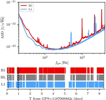
In this analysis, we use data from the two aLIGO detectors in Hanford, Washington(H1) and Livingston, Louisiana (L1). No data from Virgo(Acernese et al. 2015) or GEO600(Dooley et al.2016) was used because of their lower sensitivity.171Three of the pipelines use data up to 2 kHz, while STAMP also uses data up to 4 kHz. Both detectors in their O2 configuration had their best sensitivity in the 100–200 Hz range, with significantly less sensitivity in the kHz range (e.g., a factor ∼4 worse in strain at 2 kHz)—see Figure1. For the lower analysis cutoff of each pipeline, see Section4.
Starting from a rounded GW170817 coalescence time of tc»1187, 008, 882 s, the HMM pipeline uses 9688 s of data (until the first gap in H1 data), ATrHough uses 1 day of data after tc, FreqHough analyzes from 1 to about 18 hr after tcin different configurations, and STAMP analyzes the whole 8.5 days of data until the end of O2 on 2017 August 26. The duty cycle of both detectors(H1, L1) was 100% during the first 9688 s after the merger, (70%, 78%) for the first day (62% in coincidence), and (83%, 85%) for the full dataset (75% in coincidence). The analyzed data segments are also illustrated in Figure1. STAMP processes the h(t) strain data into cross-power time-frequency maps(see Section4.1for details), while the basic analysis units of the other pipelines are Short Fourier Transforms(SFTs) of 1–8 s duration.
Several known noise sources have been subtracted from the strain data using a new automated procedure(Davis et al. 2019) that has been applied to the full O2 dataset, which processes a much larger amount of time than the cleaning method(Driggers et al. 2019) that was used for the shorter
datasets analyzed in previous GW170817 publications. Cali-bration uncertainties(Cahillane et al.2017) for this dataset are estimated as below 4.3% in amplitude and 2°.3 in phase for 20–2000 Hz, and 4.5% in amplitude and 3°.8 in phase for 2–4 kHz—which are tighter than for the initial calibration version used in Abbott et al.(2017g). These uncertainties are not explicitly propagated into the sensitivity estimates presented in this paper because they are smaller than other uncertainty contributions and the degeneracies in amplitude parameters.
4. Search Methods and Configurations
In this section, we briefly describe the four search methods, first the unmodeled STAMP and HMM pipelines and then the two Hough pipelines tailored to the power-law spindown model. Additional details can be found in AppendixA.
Each analysis uses the known sky location of the counterpart near R.A.=13.1634 hr, decl.=−23°.3815 (Abbott et al. 2017e; Coulter et al. 2017), but makes different choices for the analyzed data span. The recovery efficiency of each algorithm is studied with simulated signals under the waveform model from Section 2, as described in Section 5 and AppendixB.
A summary of configurations for all four pipelines, both for the main search and the sensitivity estimation simulations, is given in Table1.
4.1. STAMP
STAMP(Thrane et al. 2011) is an unmodeled search pipeline that is designed to detect gravitational wave transients. Its basic unit is a spectrogram made from cross-correlated data between two detectors. Narrowband transient gravitational waves produce tracks of excess power within these spectro-grams and can be detected by pattern-recognition algorithms. Each spectrogram pixel is normalized with the noise to obtain a signal-to-noise ratio(S/N) for each pixel.
STAMP was used in the first GW170817 post-merger search(Abbott et al.2017g) in a configuration with 500 s long spectrograms. To increase sensitivity to longer GW signals, here we use spectrogram maps of 15,000 s length. The search is split into two frequency bands from 30 to 2000 and 2000 to 4000 Hz. The former uses pixels of 100 s´1 Hz, while the latter uses shorter-duration pixels of 50 s´1 Hzto limit S/N loss due to the Earth’s rotation changing the phase difference between detectors.
We then use Stochtrack(Thrane & Coughlin2013), which is a seedless clustering algorithm, to identify significant clusters of pixels within these maps. The algorithm uses one million quadratic Bézier curves as templates for each map and the loudest cluster is picked for each map. More details about the pixel size choice, the detection statistic and the search results are given in AppendixA.1.
The on-source data window is from just after the time of the merger to the end of O2 (1187008942–1187733618). To measure the background and estimate the significance of the clusters that we have found, we run the algorithm on time-shifted data from June 24th to just before the merger.
4.2. HMM Tracking
Hidden Markov model (HMM) tracking provides a
computationally efficient strategy to detect and estimate a
Figure 1.Top panel: noise strain amplitude spectral density(ASD) curves of LIGO Hanford(H1) and Livingston (L1) on 2018 August 17. (Averaged over 1800 s stretches including GW170817.) Lower panel: analyzable science mode data segments for the remaining O2 run after the GW170817 event. Vertical-dotted lines mark the analysis end times, from left to right, for HMM, FreqHough, ATrHough and STAMP.
171
For example, at 500 Hz the noise strain amplitude spectral density was about a factor of∼5 for Virgo and ∼20 for GEO600 worse than for L1 in late O2.
quasimonochromatic GW signal with unknown frequency evolution and stochastic timing noise(Suvorova et al.2016; Sun et al.2018). It was applied to data from the first aLIGO observing run to search for CWs from the low-mass X-ray binary Scorpius X-1(Abbott et al.2017f). The revision of the algorithm in Sun et al.(2018) is also well-suited to searching for a long-transient signal from a BNS merger remnant, if the spin-down timescale is in the range 10 s2 t 10 s4 .
A HMM is an automaton that is based on a Markov chain(a stochastic process transitioning between discrete states at discrete times), which is composed of a hidden (unmeasurable) state variable and a measurement variable. A HMM is memoryless; i.e., the hidden state at time tn+1 only depends on the state at time tn, with a certain transition probability. The
most probable sequence of hidden states given the observations is computed by the classic Viterbi algorithm (Viterbi 1967). Further details on the probabilistic model can be found in AppendixA.2.
In this analysis, we track the GW signal frequency as the hidden variable, whose discrete states are mapped one-to-one to the frequency bins in the output of a frequency-domain estimator computed over an interval of length Tdrift. We aim to search for signals with 10 s2 t 10 s4 , such that thefirst time derivative f˙gw of the signal frequency fgwsatisfies f˙gw» fgw t1 Hz s-1, given Tdrift=1 sand a frequency bin width ofD =f 1 Hz. The motion of the Earth with respect to the solar system barycenter (SSB) can be neglected during a Tdrift interval. Hence, we use a running-mean normalized power in SFTs with length TSFT=Tdrift=1 s as the estimator to calculate the HMM emission probability.
We analyze 9688 s of data (GPS times 1187008882– 1187018570) in a 100–2000 Hz frequency band with multiple configurations optimized for different τ. We do not analyze longer data stretches because: (i) several intervals in the data after GPS time 1187018570 are not in analyzable science mode, and (ii) signals with 10 s2 t 10 s4 drop below the algorithm’s sensitivity limit after 10 s~ 4 . Observing for longer merely accumulates noise without improving S/N. The 9688SFTs are Hann-windowed. The detection statistic is
defined in Equation (17). The methodology and analysis is fully described in Sun & Melatos(2018).
4.3. Adaptive Transient Hough
The Adaptive Transient Hough search method is described in detail in Oliver et al. (2019). It follows a semi-coherent strategy similar to the SkyHough(Krishnan et al.2004; Sintes & Krishnan2007; Aasi et al. 2014) all-sky CW searches, but adapted to rapid-spindown transient signals.
We start from data in the form of Hann-windowed SFTs with lengths of[1, 2, 4, 6, 8] s, covering one day after merger (GPS times 1187008882–1187095282). These are digitized by setting a threshold of 1.6 on their normalized power, as first derived by Krishnan et al. (2004), replacing each SFT by a collection of zeros and ones called a peak-gram. For each point in parameter space, the Hough number count is the weighted sum of the peak-grams across a template track accounting for Doppler shift and the spindown of the source. The use of weights minimizes the influence of time-varying detector antenna patterns and noise levels(Sintes & Krishnan 2007). For this post-merger search, it also accounts for the amplitude modulation related to the transient nature of the signal.
The search parameter space for the model from Section 2 covers a band of 500–2000 Hz in starting frequencies fgw0, braking indices of 2.5 n 7 and spindown timescales of 102 t 10 s5 . The search runs over 16,042 subgroups, each containing a range of 150 Hz in f0, 0.25 in n and 1000 s in τ.
Each subgroup is analyzed with the longest possible SFTs according to the criterion(Oliver et al.2019)
T n f 1 , 5 SFT gw ( - )t ( )
and for each template the observation time is selected as Tobs=min 4 , 24 hr( t ). Over the whole template bank, the search uses data from 187 to 2000 Hz.
Each template is ranked based on the deviation of its weighted number count from the theoretical expectation for Gaussian noise
Table 1
Configurations of the Four Analysis Pipelines Used in This Paper
STAMP HMM ATrHough FreqHough
Search starta tc tc tc tc+ (1–7) hrb
Search duration(hr) 201.3c 2.7 24 2–18b
fgwdata range(Hz) 30–4000c 100–2000 187–2000 50–2000
n coverage unmodeled unmodeled 2.5–7.0 2.5–7.0
fstartcoverage(Hz)d unmodeled unmodeled 500–2000 500–2000
τ coverage (s) unmodeled unmodeled 102–105 10–105
injection set for sensitivity estimatione
Signal starta random tc tc tc+ [1, 2, 5] hrb
n coverage 5.0 2.5–7.0 5.0 5.0
fstartcoverage(Hz)
d
500–3000 500–2000 550–2000 390–2000
τ coverage (s) 102–104 102–104 6×10²–3×10⁴ 4×10²–2×10⁴
Inclination cos i 0.0, 1.0 random 0.0, 1.0 random
Notes.
a
Coalescence time tc»1187, 008, 882rounded to integer GPS seconds.
b
FreqHough search start and duration vary across parameter space.
c
In separate maps of 15,000 s length and 20–2000 and 2000–4000 Hz configurations.
d
fstart =fgw(t=0) for HMM and ATrHough; fstart =fgw(t= Dt) for STAMP and FreqHough.
(the critical ratio) as described in Appendix A.3. The detection threshold corresponds to a two-detector 5σ false-alarm prob-ability for the entire template bank. A per-detector critical ratio threshold was also set to check the consistency of a signal between H1 and L1.
4.4. Generalized FrequencyHough
The FrequencyHough is a pattern-recognition technique that was originally developed to search for CWs by mapping points in time-frequency space of the detector to lines in frequency-spindown space(Antonucci et al.2008; Astone et al.2014). This only works if the signal frequency varies in time very slowly. Miller et al. (2018) have generalized the FrequencyHough for post-merger signals, where we expect much higher spindowns.
The search starts at a time offset D =t tstart-tc after coalescence time tc, so that the waveform model is interpreted with starting frequency fstart =fgw(t= Dt) taking the place of fgw0in Equation(3). In this way, assuming that the NS has already spun down before tstart following some arbitrary track, we would be able to probe higher initial frequencies and spindowns through a less challenging parameter space during the search window. Furthermore, the source parameters n f( , start,t) are transformed to new coordinates, such that in the new space the behavior of the signal is linear. See AppendixA.4for the transformation relations. We search across the parameter space with afine, nonuniform grid: for each braking index n, we do a Hough transform and then record the most significant candidates over the parameter range of the resulting map. This is done separately on the data from each detector. We then check the candidates for coincidence between detectors according to their Euclidean distance in parameter space. The search is run in three configurations using varying TSFT=2, 4, 8 s, covering different observing times, starting
t 1 7
D = – hr after merger. It covers n= [2.5, 7], fstart = 500, 2000
[ ] Hz and t = [10, 105] , analyzing detector datas from 50 to 2000 Hz.
Candidates are also ranked by critical ratio (deviation from the theoretical expectation for Gaussian noise) in this analysis. Most can be vetoed by the coincidence step or by considering detector noise properties. A follow-up procedure for surviving candidates is also described in AppendixA.4.
5. Search Results and Sensitivity Estimates 5.1. Absence of Significant Candidates
All of the four search methods either found no significant candidates in the aLIGO data after GW170817; or those that were found, were clearly vetoed as instrumental artifacts.
For the unmodeled STAMP search, the loudest triggers in the low- and high-frequency bands have S/Ns of 3.18 and 3.07, respectively. The time-shifted backgrounds only just start to drop off near these S/Ns, so that they correspond to false-alarm probabilities pFAof 0.81 and 0.80, which are completely consistent with noise. For reference, pFA =0.05 would only have been reached for S/Ns of 4.9 and3.5for these low-and high-frequency background distributions, respectively. (See Figure4 in AppendixA.1.)
For HMM, the loudest trigger has a detection statistic 2.6749
= (as defined in Equation (17)), which corresponds to a false-alarm probability of 0.01, right below the threshold set beforehand as significant enough for further study. The trigger is found with observing time Tobs=200 sstarting from t= . Monte-Carlo simulations show that for the signals thattc
this setup is sensitive to, a higher should be obtained with longer Tobs. Follow-up analysis of the trigger with 300 s Tobs1000 sconfirms that it does not follow this expectation; hence, it is discarded as spurious.
ATrHough found 51 initial candidates over the covered part of n f( , gw0,t) parameter space. All of these were excluded with the follow-up procedure described in Appendix A.3 because they are inconsistent with the expected spindown model and are more likely to have been caused by monochromatic detector artifacts(lines) contaminating the search templates.
The FreqHough search returned 521 candidates over the covered part of n f( , start,t) parameter space. We vetoed 10 of them because they were within frequency bands contaminated with known noise lines(Covas et al.2018). A total of 510 of the remaining candidates had much higher ( 4> times) critical ratios in H1 than in L1, which is inconsistent with true astrophysical signals when considering the relative sensitiv-ities, duty factors and antenna patterns. There was one remaining candidate, with a critical ratio of 5.21 in H1 and 4.88 in L1, which was followed up and excluded with the procedure described in AppendixA.4.
5.2. Sensitivity Estimates with Simulated Signals Starting from this non-detection result, we use simulated signals according to Equation(3) to quantify the sensitivity of each analysis given the dataset around the time of GW170817 and its known sky location. The sets of injected parameters are different for each pipeline, while there are also some differences in procedure: STAMP performs injections on the same data as the main search but with a non-physical time shift between the detectors(as in Abbott et al.2017g,2018a); HMM injects signals into the original set of SFTs but with randomly permuted timestamps; and the other two pipelines inject signals into exactly the same data as analyzed in the main search. HMM and ATrHough perform all injections starting at merger time tc, with fgw0in Equation(3) interpreted as the frequency at tc, while injections for FreqHough are done atD =t 1, 2 or 5 hr after tc, which are chosen as representative starting times for each search configuration, and fgw0is correspondingly set at tc+ D . Similarly, STAMP treats ft gw0as the starting frequency of each injection, which haveD distributed through the wholet search range, yielding a time-averaged sensitivity. In the following, we use fstartto refer to any of these choices.
These differences in injection procedure and the different choices of detection threshold mean that any comparison of the following results does not correspond to a representative evaluation of general pipeline performance but is solely in the interest of estimating how much sensitivity is missing for a GW170817-like post-merger detection that is based on the specific configurations that are used in the present search.
We focus here on results for a braking index of n=5, as expected for spin-down dominated by GW emission from a static quadrupole deformation. The signal amplitude h0 (as given in
Equation(4)) is degenerate between the ellipticity ò, moment of inertia Izz and distance d. We choose a fiducial value of Izz=
M G c
100 3 2 4»4.34´1038kg m2
, which is consistent with
EoS yielding a supramassive or stable remnant: the high mass and assumed rapid rotation can increase the moment of inertia by more than a factor of 3 compared to a nonrotating NS of1.4M. In addition, EoS compatible with the high remnant mass favor larger moments of inertia already at lower mass. For a given set of
model parameters n{ =5,fstart,t}, we consider the maximumò allowed by the initial rotational energy budget(Sarin et al.2018): the total emitted GW energy as t ¥,
E dt G c I t 32 5 , 6 t t zz gw 5 2 2 6 start
ò
= - W = ¥ ( ) ( )must not exceed the remnant’s initial rotational energy Erot= I f
0.5 zz start2 p .2
Given each pipeline’s detection threshold, we can rescale the amplitude of simulated signals until 90% of them are recovered above threshold, while randomizing over nuisance parameters (polarization angle and initial phase of the signal; also source inclinationι and signal start time for some of the pipelines). We can then either interpret this amplitude scaling as a need to lower the distance of simulated sources; i.e., estimating the sensitive distance d90%of the search. Alternatively, we canfix the true distance to the source of GW170817 to obtain an energy upper limit Egw90%: for a remnant NS with the given
parameters, we interpret the square of the amplitude scaling as the factor by which the energy output needs to be greater than the expected amount to produce signals that we can recover at 90% confidence. Both interpretations are shown in Figure 2, with coverage of the injection sets illustrated in Figure3. The full results are listed in the appendix in Tables2–5.
The highest sensitivities are achieved at low fstart and for rapid spindown (low τ). This is mostly due to the energy budget constraint enforced onò: in principle, higher fstart yield higher initial amplitudes and longer τ allow accumulation of S/N over longer observation times (S Nµt1 2for n=5 and once Tobs> ). However, due to the energy budget constraint, òt must be lower in this region of parameter space and hence actual detectability is reduced(S N 1f
start 6
t
µ µ - - ).
The four pipelines perform differently across τ regimes: the unmodeled STAMP and HMM are most sensitive at the shortest
102
t = s, but lose up to an order of magnitude in d90%when going to t =10 s4 . Meanwhile, the model-based semi-coherent Figure 2.A sample of search sensitivities achieved for the power-law spindown signal model with braking index n=5. Results are shown as sensitive distance d90%
(left-hand panel) for otherwise physical parameters, or as required emitted energy Egw90%at afixed distance d=40 Mpc (right-hand panel), both as a function of reference starting
frequency fstartused for the injections of each pipeline.(fstart =fgw(t= Dt) for STAMP and FreqHough and fstart =fgw0 =fgw(t=0) for the others.) See Figure3for the parameter ranges covered by each injection set. Thisfigure shows the subset with highest sensitivity for each analysis; this corresponds to the shortest (t =100s) injections for STAMP and HMM, while for ATrHough and FreqHought (fstart) is variable, depending on the search coherence length, as also listed in Tables4and5. Note that detection
thresholds are also different between pipelines. The NS ellipticityò is always chosen as the maximum allowed by the energy budget constraint Egw=Erotat each(n f, start,t)
parameter point, assuming a NS moment of inertia of Izz=100M G3 2 c4»4.34´1038kg m2. Injections were randomized over source inclination cos i for HMM and FreqHough, while for STAMP and ATrHough injections for the best case(cosi = ) and worst case (cos1 i = ) are shown separately. For comparison, the known distance to0 the source of GW170817 is indicated by a horizontal dashed line in the left-hand panel, as well as two(optimistic) energy upper limits in the right-hand panel: the total system energy(dotted line, using a fiducial value of Etot=3.265M c 2as in Abbott et al.2017g) and the initial rotational energy Erot as a function of fstart(dashed line).
Figure 3.Parameter coverage in fstart,τ and ò of the injection sets used for the n=5 sensitivity estimates, as listed in Tables2–5. As shown in the left-hand panel, the
HMM and STAMP injections are atfixedt Î [10 , 10 , 102 3 4] s, while for ATrHough and FreqHough different f start
t ( ) curves are covered for different choices of TSFT
(and, in the case of FreqHough, tD ) in the search setup. At each n f( , start,t) parameter space point, the maximumò allowed by the energy budget (Egw=Erot) is
chosen(right-hand panel), assuming a NS moment of inertia of Izz=100M G3 2 c4»4.34´1038kg m2. Lines of constantò (left panel) or τ (right-hand panel) are shown for comparison. STAMP injections include fstartup to 3000 Hz for longerτ, with those above 2000 Hz covered by the high-frequency search configuration. But
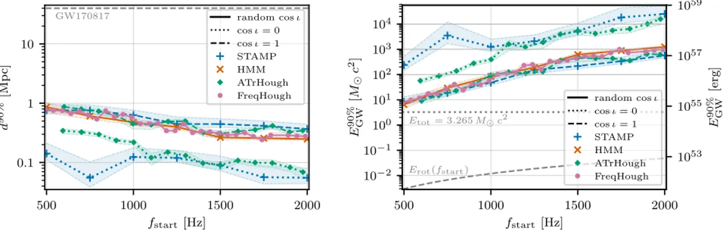

![Figure 6. STAMP 90% sensitivity estimates for n =5 and variable f start . For either cos i = [ 0, 1 ], the connected lines (from top to bottom in d) are for injections with 10 , 10 , 1023 4](https://thumb-eu.123doks.com/thumbv2/123dokorg/5402638.58036/17.918.98.823.80.255/figure-stamp-sensitivity-estimates-variable-start-connected-injections.webp)
