Comparison and sensitivity analysis of marine CSEM exploration methods

(1)

I

POLITECNICO DI MILANO

School of Civil, Environmental and Land Engineering Master of Science in Environmental and Geomatic Engineering

Comparison and sensitivity analysis of marine CSEM exploration methods

Master Dissertation by

Babak Taleghani

Supervisor

Prof. Giancarlo Bernasconi

(2)

I

(3)

II

Acknowledgement

I would first and foremost like to thank my supervisor, Prof. Giancarlo Bernasconi, who offered me such a great opportunity to study in the Applied Geophysics, Department of Electronic and information, Politecnico Di Milano. I am grateful to him for his assistance and his great ability to lucidly explain the most difficult concepts to me. I thank him for his time, his constant encouragement and for always enlightening the positive side of a situation. I deeply appreciate his full support for providing invaluable assistance that ultimately made this thesis a reality. With regards to research, he has always insisted that I try to find worthwhile questions to answer.

I would like to thank prof. Gentili for his generous help for introducing me to the world of Sensitivity analysis.

Of course, I must also express my gratitude to the entire Electronic and information Department of Politecnico Di Milano. In particular, I am grateful to Andrea Gola for all fruitful discussions we had.

Moreover, I would like to thank the many people from whom I learnt over the years; in particular, Prof. Dr. Toraj Mohammad and Eng. Mohammad Samei who taught me a great deal about looking at modelling process and interpreting data.

Also deserving special thanks to Ahmad Abedi, and my Uncle, Abbas Sanjari who were extremely kind and supportive during my study at Politecnico Di Milano. I would like to offer another special thanks to Sepehr Marzi for his full academic support.

I would like to express my gratitude to my parents who supported me over the years and encouraged me to keep going, I am forever indebted for their full kindest support in every single step of my life.

(4)

III

FIGURE 5.SCHEMATIC REPRESENTATION OF THE HORIZONTAL ELECTRIC DIPOLE-DIPOLE MARINE CSEM METHOD.AN ELECTROMAGNETIC TRANSMITTER IS TOWED CLOSE TO THE SEAFLOOR TO MAXIMIZE THE COUPLING OF ELECTRIC AND MAGNETIC FIELDS WITH SEAFLOOR ROCKS.THESE FIELDS ARE RECORDED BY INSTRUMENTS DEPLOYED ON THE SEAFLOOR AT SOME DISTANCE FROM THE TRANSMITTER.SEAFLOOR INSTRUMENTS ARE ALSO ABLE TO RECORD MAGNETOTELLURIC FIELDS THAT HAVE PROPAGATED DOWNWARD THROUGH THE SEAWATER LAYER ... 18

FIGURE 6.SCHEMATIC PRESENTATION OF THE ACQUISITION SYSTEM BASED ON CURRENT INJECTION USING A VERTICAL BIPOLE AND REGISTRATION OF THE VERTICAL COMPONENT OF THE ELECTRIC FIELD.THE INJECTED CURRENT IS SWITCHED OFF AT T ¼0. PARAMETERS HS, HO, HT INDICATE THE WATER DEPTH, THE OVERBURDEN, AND RESERVOIR THICKNESSES; ΡS, ΡO, ΡU, ΡT ARE THE WATER, OVERBURDEN, UNDERBURDEN, AND RESERVOIR RESISTIVITIES; W SPECIFIES THE HORIZONTAL EXTENT OF THE RESERVOIR.THE CASE OF W ¼0 CORRESPONDS TO A STRATIFIED STRUCTURE WITHOUT A RESERVOIR; THE CASE OF W ¼∞ CORRESPONDS TO A STRATIFIED STRUCTURE WITH THE RESERVOIR UNLIMITED IN BOTH HORIZONTAL DIRECTIONS ... 19

FIGURE 7.AN OVERVIEW OF THE PETROMARKER TECHNOLOGY (NOT TO SCALE), ONLY ONE PULSE SYSTEM IS SHOWN.THE UPPER AND LOWER PULSE ELECTRODES WHICH ARE DIRECTLY ON TOP OF EACH OTHER FORM THE VERTICAL TRANSMITTER DIPOLE, THE RETURN CURRENT GOES THROUGH THE SEA.TO THE LEFT ON THE SEA BOTTOM, THE EXTENSIBLE TRIPOD IS SHOWN, AND TO THE RIGHT, A FLEXIBLE CABLE RECEIVER.THE COLOUR SCALE (UNIT LOG10(|EZ|(IN V/M)) OF THE SEDIMENTS REPRESENTS THE VERTICAL ELECTRIC FIELD IN THE PRESENCE OF THE HC-FILLED RESERVOIR (YELLOW).THE ELECTRIC FIELD IS EVALUATED FOR A 5000AM SOURCE DIPOLE SHORTLY BEFORE THE CURRENT IS TURNED OFF. ... 21

FIGURE 8.A SKETCH OF THE TOWED-STREAMER EM SYSTEM. ... 22

FIGURE 9.SENSITIVITY MAPS OF THE CSEM METHOD FOR DEEP TOWING (TOP) AND SURFACE TOWING FOR A =5%(MIDDLE) AND A =3%(BOTTOM).THE SENSITIVITY IS DEFINED AS THE TARGET RESPONSE NORMALIZED TO UNCERTAINTY,EQ.1.THE SURFACE TOWING PROVIDES EQUAL OR BETTER SENSITIVITY IF THE WATER DEPTH IS SMALLER THAN 450 M.REDUCTION IN THE NAVIGATION UNCERTAINTY (A =3%) MOVES THE THRESHOLD DEPTH TO 700 M.TARGET DEPTH IS 2 KM. ... 24

FIGURE 10.SCHEMATIC REPRESENTATION OF INVERSE MODELING (SNIEDER, ET AL.,1999) ... 27

FIGURE 11.THE AIRWAVE.THE NORMALIZED IMPULSE RESPONSES OF THE MODELS IN (A) AND (B) TO AN ELECTRIC DIPOLE–DIPOLE SYSTEM ON THE SEAFLOOR ARE SHOWN AS FUNCTIONS OF LOGARITHMIC TIME AND TRANSMITTER RECEIVER SEPARATION. PANELS (C) AND (D) REFER TO INLINE AND PANELS (E) AND (F) TO BROADSIDE GEOMETRIES. ... 29

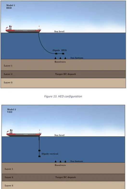
FIGURE 13.HED CONFIGURATION ... 33

FIGURE 14.VED CONFIGURATION ... 33

FIGURE 15.TSEMCONFIGURATION ... 34

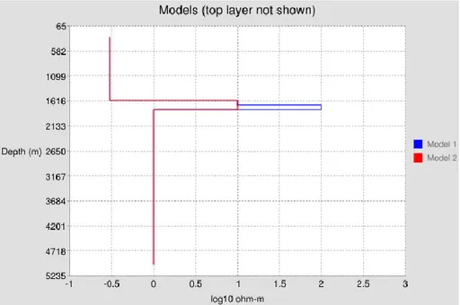
FIGURE 16.RESISTIVITY MODEL... 35

TABLE 1.MODEL WITH HYDROCARBON DEPOSIT IN DEPTH OF 1700M BELOW THE SEA WATER ... 36

TABLE 2.MODEL WITHOUT HYDROCARBON DEPOSIT IN DEPTH (HOMOGENOUS MEDIUM) ... 36

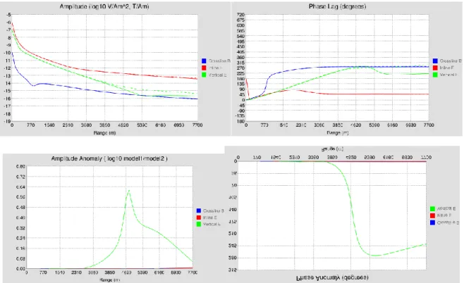
FIGURE 17MAGNITUDE VERSUS OFFSET (MVO) AND PHASE VERSUS OFFSET (PVO) WITH FREQUENCY OF 0.20HZ ... 37

FIGURE 18.MAGNITUDE VERSUS OFFSET (MVO) AND PHASE VERSUS OFFSET (PVO) WITH FREQUENCY OF 0.48HZ ... 37

(7)

VI

FIGURE 29.REGULARIZATION WITH DATA AND MODEL RELIABILITY ... 45

FIGURE 30.RESISTIVITY MODEL PROFILE OF CSEM ATTRIBUTE FOR DIFFERENT FREQUENCIES. ... 46

FIGURE 31.INVERSION MODEL PARAMETERS ... 47

FIGURE 32.RESULT OF EX AND HY AND PHASE AND FIELDS FOR INVERTED MODEL ... 48

TABLE 3.INVERTED RESISTIVITY MODEL OF FAROE ISLAND ... 49

FIGURE 33.CONDUCTIVITY ANALYSIS OF INVERSION MODEL ... 49

FIGURE 34.SENSITIVITY PLOT OF HED WITH FREQUENCY OF 0.20HZ... 53

FIGURE 35.SENSITIVITY PLOT OF HED WITH FREQUENCY OF 0.48HZ ... 54

FIGURE 38.SENSITIVITY PLOT OF VED WITH FREQUENCY OF 0.20HZ ... 55

FIGURE 39..SENSITIVITY PLOT OF VED WITH FREQUENCY OF 0.48HZ ... 56

FIGURE 42.SENSITIVITY PLOT OF TSEM WITH FREQUENCY OF 0.20HZ ... 57

FIGURE 46.SENSITIVITY COMPARISON WITH RESPECT TO FREQUENCY (HED) ... 62

FIGURE 47.SENSITIVITY COMPARISON WITH RESPECT TO FREQUENCY (VED) ... 62

FIGURE 48.SENSITIVITY COMPARISON WITH RESPECT TO FREQUENCY (TSEM) ... 63

FIGURE 49.EX LAYER RESPONDED AT 0.20HZ (TSEM) ... 64

FIGURE 46.EZ LAYER RESPONDED AT 0.20HZ (VED) ... 64

FIGURE 50.EX LAYER RESPONDED AT 0.20HZ (HED) ... 64

FIGURE 51.1D MODEL GEOMETRY.THERE ARE N-LAYERS WITH RESISTIVITY 𝜌 IN UNITS OF OHM-M.EACH LAYER IS DEFINED IN TERMS OF THE ABSOLUTE DEPTH OF THE TOP OF THE LAYER IN UNITS OF METERS.RECEIVERS AND TRANSMITTERS CAN BE LOCATED ANYWHERE IN THE STACK OF LAYERS. ... 65

FIGURE 52.TRANSMITTER ORIENTATION PARAMETERS.THE TRANSMITTER AZIMUTH IS DEFINED TO BE THE HORIZONTAL ROTATION OF THE TRANSMITTER ANTENNA FROM THE X AXIS, POSITIVE TOWARDS Y.SO AN AZIMUTH OF 0 MEANS THE ANTENNA POINTS ALONG X, WHILE AN ANGLE OF 90 DEGREES MEANS THE ANTENNA POINTS ALONG Y.THE TRANSMITTER DIP ANGLE IS POSITIVE DOWN FROM THE AZIMUTH ANGLE. ... 66

FIGURE 53.CSEM CONVENTION FOR DATA PROCESSING ... 67

List of Tables

TABLE 1.MODEL WITH HYDROCARBON DEPOSIT IN DEPTH OF 1700M BELOW THE SEA WATER ... 36

TABLE 2.MODEL WITHOUT HYDROCARBON DEPOSIT IN DEPTH (HOMOGENOUS MEDIUM) ... 36

(8)

VII

Symbols and Notations

𝜎 ……….. .. Bulk conductivity ∅ ……….. Porosity 𝜇 ……….. Magnetic permeability 𝜀 ……… dielectric permittivity 𝜌 ……… Density 𝜌_𝑟………... Resistivity J ……… Matrix of Jacobean MVO ………. Magnitude vs. off-set PVO ……… Phase vs. Off-set E ……… Electric field intensity B ……… Magnetic flux density 𝜏 ……… Characteristic diffusion time

(9)

VIII

Abstract

Hydrocarbon deposits in the form of petroleum, natural gas, and natural gas hydrates occur offshore worldwide. Electromagnetic methods that measure the electrical resistivity of sediments can be used to map, assess, and monitor these resistive targets. In particular, quantitative assessment of hydrate content in marine deposits, which form within the upper few hundred meters of seafloor, is greatly facilitated by complementing conventional seismic methods with EM data.

In this study we developed comparison test between the acquisition configurations, VED, HED and TSEM one-dimensional reservoir response to the diffusive EM field.

This thesis explores the comparison and sensitivity analysis of Marine CSEM data with respect to the more important acquisition Configurations (VED, HED and TSEM), namely with different frequencies (0.2Hz, 0.48Hz, 0.76Hz, 1.04Hz) based on 1D – forward modeling. This analysis helps the interpreters to highlight the reliability of each acquisition method parameter in a complex CSEM inversion and gives them the idea to select the more efficient method for CSEM survey according to geometry of hydrocarbon deposit.

Keywords: Marine Controlled Source Electromagnetic (M-CSEM), Sensitivity Analysis,

Forward modelling, Vertical electric dipole (VED), Horizontal electric dipole (HED), Towed source EM (TSEM)

(10)

1

Chapter 1 Introduction to Marine Controlled Source EM

(CSEM) For Hydrocarbon Deposit Exploration

(11)

2

1.1 Brief Background of Hydrocarbon Deposit Exploration

Measurements of electrical resistivity beneath the seafloor have traditionally played a crucial role in hydrocarbon exploration (Eidesmo, et al., 2002). Electromagnetic (EM) sounding methods represent one of the few geo scientific techniques which can provide information about the current state and properties of the deep continental crust and upper mantle (Boerner, 1992). As the industry’s search for hydrocarbon resources intensifies, more geoscientists are relying on these electromagnetic fields to probe areas that are difficult to image with seismic methods. The study of electrical currents in the Earth, called tellurics, is not new, first reported combining a measurement of electric and magnetic fields, termed magnetotellurics (MT), for exploration of the Earth’s subsurface in 1952.2 However, MT has become an important tool for explorationists in the E&P industry only within the past few years—thanks to advances in 3D modeling and inversion technology. Now, MT results can be combined more efficiently with seismic and gravity surveys, resulting in a more calibrated model of the earth (James Brady, et al. 2009). At the start of the 21st century, the use of CSEM expanded from onshore mining exploration into new applications for hydrocarbon exploration, initially in deep water (500 m or more) and, more recently, in shallower water (less than 500 m). The basic idea behind the use of CSEM for hydrocarbons is to identify resistive layers in an otherwise conductive environment. Charlie Cox, Professor of Geophysics at Scripps Institution of Oceanography, initiated and conducted the original academic research and developed early marine EM equipment some 25 years ago. The main focus of his work was in the field of crustal and deep ocean trench studies.

By 2000, Statoil and a major U.S. oil company (MUOC for short) were evaluating the CSEM method and its application in oil and gas exploration. Statoil had the first new CSEM survey performed offshore Angola, West Africa. The survey used existing Scripps receivers and Southampton's EM source and, although the data recorded were of relatively low resolution compared with the quality of data now being recorded 3.5 years later (10-13 against 10-15 today), the survey was a technical success. This effort proved that the CSEM method could be used for commercial oil exploration. Since then several major oil companies have invested significantly in appraisal and exploration application in this new technology and three service companies are now actively using and developing the technique in a variety of basins around the world (Steven Constable and Leonard J. Srnka, 2007).

(12)

3

1.2 Physical Properties and Behaviors

1.2.1 Geologic Properties

In order to discuss the nature of EM methods, it is useful to discuss the natural properties that affect the method. The property of interest is electrical conductivity and is related to the fluid-bearing rocks, here typically water saturated sedimentary units, through Archie's Law (Archie, 1942). The version of Archie's Law typically used in the hydrocarbon industry for brine and gas Filled sandstones:

𝜎 = 𝑎𝜎_𝑓𝑆𝑛_∅𝑚

𝜎 Is the bulk conductivity of the sample, a is tortuosity factor varying by rock type, 𝑆 is the fraction of fluid (typically water) in the pores, 𝜎𝑓 conductivity of fluid, 𝑛 is the water saturation coefficient along with 𝑚 the cementation coefficient (both typically between 1 and 2), and ∅ is the porosity

(Volume fraction of pore space). Pores can be filled by various mixtures of fluids or even air. It can be seen that this equation is dependent only on _f and not on the conductivity of the rock mineral.

Therefore, the assumption is that the more conductive fluid (by order of magnitude) dominates the bulk conductivity.

A large factor affecting electrical properties is permeability, or how well the pores are connected.

This is represented by the cementation coefficient. A formation may have high porosity (large fraction of pore space), with low permeability, or vice versa. In hydrocarbon exploration, low permeability are typically found in sedimentary units with small grain sizes, such as shales.

In mineral exploration conductive veins, dykes, or even massive sulphide bodies of various geometries may be of interest, and may be more affected by joint and fracture sets over pore spaces.

Differences between maximum permeability and minimum permeability can also be modeled using

Hashin-Shtrikman bounds (Hashin and Shtrikman, 1963), in which a two-phase conductivity model of different pore geometries are used (max and min m values).

The ocean floor above hydrocarbon bearing formations typically consists of unconsolidated sediments of up to 60% porosities in which pore spaces are filled with seawater. The cementation coefficient for the same marine sediments are usually between 1.4-1.8. This

(13)

4

gives resistivity of 1-3Ωm. Hydrocarbon reservoirs typically have resistivity values one to two orders of magnitude higher depending on the nature of the reservoir. The resistivity of seawater varies with depth within the water column and can be measured during a survey, but a good overall average is 0.3 Ω m.

1.2.2 Petro physical Properties

In the framework of hydrocarbon exploration, several researches on rock physics are conducted by oil companies for improving their expertise on the characterization of the subsurface media. The rock physics allows us to investigate and to integrate the information carried by the several well log measurements. Following, will be introduced the rock properties (Schön J.H. 1996).

1.2.2.1 Porosity

Pores are local enlargements in a pore space system that provides most of the volume available for fluid storage. Porosity φ is defined as the ration of the volume of void or pore space Vp to the total or bulk volume of the solid matrix.

∅ = 𝑉𝑝

𝑉 = 1 −

𝑉_𝑚 𝑉

This quantity is dimensionless and is generally expressed as ratio or percentage. Porosity is the result of several geological, chemical and physical processes.

1.2.2.2 Saturation

Fluid saturation is the petro physical property that describes the amount of each fluid type, (oil, water or gas), 𝑉𝑓 in the pore space. It is defined as the fraction of the pore space occupied by a fluid phase.

𝑆_𝑓 = 𝑉𝑓 𝑉_𝑝

For a given specimen has to be verified that 𝑆_𝑂𝑖𝑙+ 𝑆_{𝑊𝑎𝑡𝑒𝑟}+ 𝑆_𝐺𝑎𝑠 = 1.0 Fluid saturation can also be expressed in percentage.

(14)

5

1.3 Marine EM Theory

The theory here is based upon the development given in Ward and Hohmann (1987). Electromagnetic fields are useful in geophysics due to their interactive nature with the medium through which they propagate (Zhdanov 2009). This interaction can be used to determine certain physical properties of rocks, that is; electrical conductivity σ, dielectric permittivity ε, and magnetic permeability μ. For forward modeling problem, the operator equation is described by (Zhdanov 2009) as

{𝐸, 𝐻} ≅ 𝐴𝑒𝑚_{{𝜀, 𝜎, 𝜇}}

Where 𝐴𝑒𝑚 is an operator of the forward electromagnetic problem (non-linear in general).The electromagnetic methods are based on the study of the propagation of electric currents and electromagnetic fields in the Earth. There are two methods that can be used;

 The direct current (D.C) methods or resistivity methods:- these considers injecting an electric current in the earth by a system of current electrodes and measuring the electrical potential with receiver electrodes; where, a low frequency current (<100 Hz) is used, to propagate inside the Earth practically like a direct current (Zhdanov 2002). The D.C surveys are used to determine the resistivity of the rocks. The resistivity of the rock provides information about the mineral content and the physical structures of rocks, and also about fluids in the rocks. However, D.C survey are limited by their failure to penetrate through resistive formations (Zhdanov 2002).

 Electromagnetic induction methods: these are based on transient field which overcomes the limitation above since transient fields easily propagates through resistors. This method in addition to resistivity provides information about magnetic permeability μ, and dielectric constant ε. Zhdanov (2002) indicates that this method can be used for ground, airborne, sea bottom and borehole observations. In this type, the receivers measures the total field formed by the primary signal in the transmitter and a scattered signal from the internal structures of the Earth.

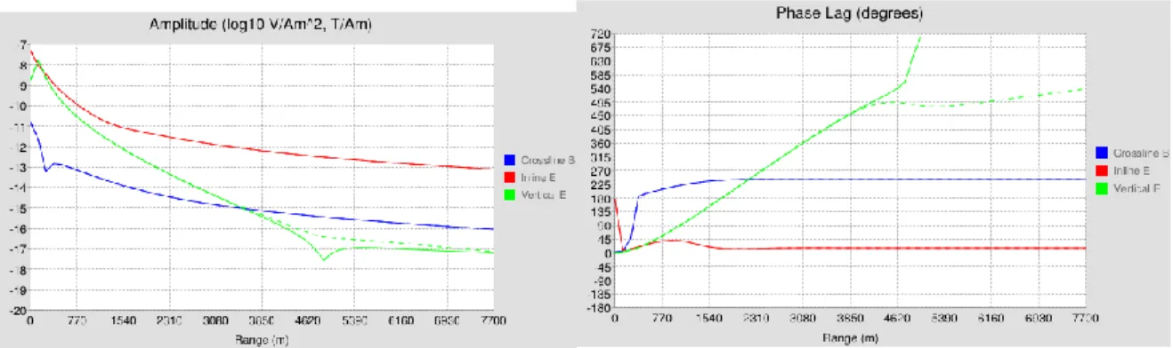
1.3.2 Amplitude and Phase

The amplitude of the secondary field is measured usually by expressing it as a percentage of the theoretical primary field at the receiver or as the resultant of the in-line and the cross-line fields. Phase shift and the time delay in the received field by a fraction of the period, can also be measured and displayed. The second method of presentation of the field is to electronically separate the received field into two components; (1) In-phase (the

(15)

6

“real”) and, (2) Out-of-phase (the “quadrature” or “imaginary”) component with the transmitted field.

In frequency domain electromagnetics, depth and size of the conductor primarily affect the amplitude of the secondary field. The quality of the conductor mainly affects the ratio of in phase to out-of-phase amplitudes.

The presence of the resistive layer results in an increased amplitude and less phase lag for both the inline and vertical components, as expected since in the resistive reservoir there is much less attenuation and phase shift of the diffusing energy than in the conductive sediments (Kerry Key , 2011).

1.3.3 Skin Depth and Penetration

The attenuation constant (skin depth) defines the rate of decay of the wave fields as the waves propagate. Skin depth is the distance over which a plane wave is attenuated by a factor of ℯ−1 in a good conductor, or as the depth at which flux density and eddy currents have decayed to ℯ−1 of their surface value. Thus the decay from the surface to the interior is exponential.

𝐸(𝑋) = 𝐸₀𝑒−𝛼𝑥

𝐸(𝛿) = 𝐸₀𝑒−𝛼𝛿 𝐸(𝛿) = 𝐸₀𝑒−1

Thus 𝛼𝛿 = 1

And from (Constable 2010), it then follows from equations above that

𝛿 = 1 𝛼 =

1 √𝜋𝑓𝜇𝜎

With f is the frequency (Hz), σ is the electrical conductivity (S/m), and μ is absolute magnetic permeability of the conductor. Due to the skin depth effect, very low frequencies (0.05-1 Hz) are applied (S. E. Johansen, H.E.F. Amundsen et al. 2005), if a deep sub-seafloor target must be penetrated. The antenna frequency affects the resolution on the E-field contrast when evaluating models with and models without hydrocarbon. The relationship between

(16)

7

any frequency and the maximum depth of detectable reservoirs (Tadiwa, Yahya et al. 2013) can be given by

𝑍_𝑚𝑎𝑥 = 600 − 851.2ln (𝑓)

Where, 𝑍𝑚𝑎𝑥 the maximum depth, and f is the antenna frequency. EM signals are rapidly attenuated in seawater (approximately 551m at 0.3 Ω-m) and seafloor sediments saturated with saline water. These signal pathways will dominate at near source-to-receiver offsets (approximately 3km) (S. E. Johansen, H.E.F. Amundsen et al. 2005).

The magnitude of the external electromagnetic noise decreases with depth, because of the skin depth effect that dampens high frequencies. Hence, the signal-to-noise ratio usually increases with water depth (Terje Holten el, al., 2009)

In the frequency domain, however, the longer skin depths associated with seafloor rocks mean that at a sufficient source-receiver distance, the field is dominated by energy propagating through the geologic formations. Energy propagating through the seawater has essentially been absorbed and is absent from the signals. Furthermore, by concentrating all the transmitter power into one frequency, larger signal-to-noise ratios can be achieved at larger source-receiver offsets Constable, S. and L. Srnka (2007).

1.4 Marine

Controlled Source EM in Practice

Controlled source EM application, an electric dipole transmitter system is deep-towed from a ship and passes a time-varying current (typically 500–1,000 A) between electrodes spaced apart by some distance (typically 100–300 m), producing an electromagnetic field that diffuses through the ocean, seafloor and air. As the EM field diffuses away from the transmitter, it is modified by the conductivity of the media it passes through. The resulting attenuation and phase shift of the transmitted EM field is recorded by an array of seafloor EM receivers containing electric field sensing dipoles and induction-coil magnetometers. Typical receivers for the 0.1–10 Hz bandwidth of most CSEM applications are based on AC - coupled electric field sensors and induction-coil magnetometers of similar design to the instrument described in Constable et al. (1998).

Marine CSEM was first used to measure the conductivity of the lithosphere (Cox 1981), while other early academic applications largely focused on detecting conductive magma chambers and hydrothermal systems at mid-ocean ridges (e.g., Young and Cox 1981; Evans et al. 1991; Sinha et al. 1998; Mac Gregor et al. 2001). Only in the past decade has it become widely recognized that the CSEM method is sensitive to thin resistive hydrocarbon reservoirs trapped in conductive sediments on the continental shelves (e.g., Edwards 2005; Constable and Weiss 2006; Um and Alumbaugh

(17)

8

2007). The first industrial field trials were carried out a decade ago using existing academic receiver and transmitter technologies to effectively detect the EM signature of a large reservoir offshore Angola (Ellingsrud et al. 2002; Eidesmo et al. 2002). Subsequently, the method was incorporated into the offshore hydrocarbon exploration toolkit in the course of only a few years (Constable 2010).

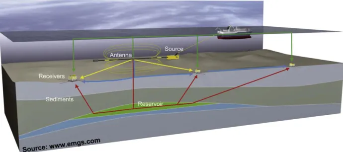
Figure 1. Schematic representation of the horizontal electric dipole-dipole marine CSEM method

The geometry in this study will be considered as an azimuth of zero-degree. Presence of a hydrocarbon causes a decrease in electrical conductivity which gives it a unique character to be easily detected. In the view point with (Eidesmo, S. Ellingsrud et al. 2002, Summerfield, Gale et al. 2005, Constable and Srnka 2007, Zhdanov 2009), the survey geometry is considered to consist of electric receivers that are placed stationary by the concrete anchors on the seabed (figure 2.). The survey design determines how well the target can be detected and characterized.

(18)

9

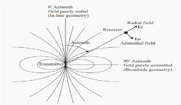
Figure 2. The geometry of CSEM dipole fields. Along the polar axis of the dipole transmitter, the field is purely radial.

Along the equatorial axis, the field is purely azimuthal. At other azimuths the received fields are a trigonometric mix of both modes (Constable and Weiss 2006).

1.4.1 Off-shore Scenario

The Marine CSEM method is particularly useful for detecting the first few percentage increases in hydrocarbon saturation at the edges of the reservoir. The electric anomalies represented by oil and gas reservoirs, which perturb the transmitted electromagnetic field, can therefore be detected in the survey data. The main goal is to determine and characterize possible thin resistive layers within the conductive surroundings beneath the seabed.

With marine CSEM now available and proven in principle, oil companies can use rock property data from well logging in appraisal, production and exploration to better understand and delineate the hydrocarbon-saturated reservoir section to which CSEM is most sensitive.

1.4.1.1 Transmitters

In the Most Marine CSEM acquisition nowadays uses a horizontal electric dipole (HED) source towed near the seabed and array of receiver dipoles on the seabed. The transmitter dipole emits a low frequency electromagnetic signal that propagates into the seawater column and downward into the subsurface (Dell'Aversana, 2007). A horizontal electric dipole,

(19)

10

is towed for several hundred meters, close to the seafloor to maximize the energy that couples to seafloor rocks (e.g., Edwards, 2005).

Some details on the CSEM transmitter:

 The streamer can be up to 300 meters long

 Electric power is transmitted to the tow vehicle along the tow cable at high voltage,

 The voltage is reduced and current increased by a transformer at the tow vehicle, and a current of up to 1000 [A] is injected into the seawater.

Although other source con-figurations have been used, such as vertical electric dipoles (VED) sources that transmit a transient electromagnetic signal when the source is turned on (Jon-Mattis Børven el, al. 2009).

VED antenna consists of two large electrodes connected to the vessel by heavy cables, The EM field is generated by sending a DC current through the lower electrode, which sits on the seabed during signal transmission, through the conductive seawater and back to the upper electrode. This electrode is lowered 30−50 m below the sea surface to minimize the influence on the EM field of the conductive hull of the survey vessel, while maximizing the transmitter dipole moment which is directly proportional to the strength of the transmitted EM field, the source signal consists of a series of pulses, each with a typical duration of 2−8s (Jon-Mattis Børven el, al. 2009).Figure 3.

Figure 3. Overview of (a) conventional horizontal-based frequency domain, CSEM, such as SBL, and (b) the recent vertical-based time domain EM method. Note the acquisition setup and diffusion paths of the transmitted and recorded signals for the two methods.

(20)

11 1.4.1.2 Receivers

The EM receivers are autonomous sea floor units deployed at pre-determined locations. Receivers are equipped with magnetic as well as electric sensors which are oriented as the three spatial coordinates, Depending on the followed approach, time or frequency domain, record the time-varying source signal over source-receiver ranges from zero to several tens of kilometers, depending upon source waveform period and the conductivity below the seafloor, receivers provide respectively the transient or magnitude and phase of the received signal over the transmitter-receiver separation, offset (P.J. Summerfield, el. Al., 2005).

Receivers located at a suitable offset (distance between transmitter and receiver) range record the amplitude and phase of the horizontal electric field components. The appropriate offset range is typically 6−10 km (Jon-Mattis Børven el, al. 2009).

1.4.2 Field Penetration

Performing a marine surveying for hydrocarbon, it is very important to estimate the penetration of the electromagnetic field, into the sub-seafloor. Here, the skin effect describes the penetration of electromagnetic fields into materials.

We remind the well-known formula:

𝛿 = √ 2

𝜇𝜔𝜎 ≈ 500√ 𝜌 𝑓

Where δ is the distance, measured in meters, at which E and H fields are both attenuate by a factor e. This result is derived from the analysis of the wave equation in frequency domain. The same result can be obtained by performing the analysis in time domain, (Nabighian M.N. el. Al. 1991). (Bostick, 1977), introduces the equivalent depth of investigation of a plane wave which is derived from asymptotic relations based on a uniformly layered half-space. The result allows to get a rough calculation of the effective depth of investigation penetration D, measured in meters, of a plane wave in a medium:

𝐷 = 𝛿

(21)

12

The electromagnetic wave propagation through the sub-seafloor, is facilitated by the particular geometry and electrical properties of the offshore scenario. The following considerations explain schematically the propagation phenomenon:

 Sea water has a skin depth bigger than distance dipole seafloor, few ten of meters, (Figure 4.1). This allows fields to diffuse through the sub-seafloor, for several thousand of meters, since the skin depth of the sub-seafloor is twice;

 The water column is larger than its skin depth, preventing the birth of airwave;

 For the previous reason, MT sources coming from the atmosphere do not reach the receivers;

 The first offset of the receiver line is widely bigger than water skin depth to prevent that direct fields reach the first receiver (Fabio Marco Miotti, 2012).

1.4.3 Resolution

Due to the low frequency used in CSEM data acquisition, the vertical resolution is poor and will limit the ability to identify the thickness of the reservoir and the possibility of several stacked targets being present. Depending on the grid resolution and inversion/ migration algorithms used, there may be restrictions to mapping lateral extent (Jonny Hesthammer, et. Al. 2010).

It is important to cover sufficiently broad frequency range in order to improve the depth resolution. The spatial resolution of the EM data is mainly limited by the noise level and receiver spacing.it is challenging to reach depths of more than 3 km below the seabed due to lower resolution and the noise level becoming higher than the real signal (Jonny Hesthammer, et. Al. 2010).

The spatial resolution of CSEM method is lower compared to seismic since extremely low frequency are involved. The resolution is determined by the intrinsic characteristic of the diffusion equation which governs the electromagnetic phenomenon of CSEM technique. However, to perform a quantitative measure of CSEM resolution is quite complicated because considerable confusion exists on this topic, (Constable, 2010. Constable S. and Srnka L.K. 2007).

We start with the damped wave equation used to describe the vector electric field E in ground-penetrating radar:

∇2_{𝐸 = 𝜇𝜎}𝜕𝐸 𝜕𝑡 + 𝜇𝜖

𝜕2𝐸 𝜕𝑡2

(22)

13

Where t is time, 𝜎 is conductivity (between 100 and 10^-6 S/min typical rocks), 𝜇 is magnetic permeability (usually taken to be the free space value of 4𝜋 *10−7H/m in rocks lacking a large magnetite content), and 𝜖 is electric permittivity (between 10−9 and 10−11 F/m, depending on water content). The first term is the loss term, and disappears in free space and the atmosphere where 𝜎 = 0, leaving the lossless wave equation that will be familiar to seismologists (Constable, 2010).

The vertical resolution of wave propagation is proportional to inverse wavelength, and a wave carries information accumulated along its entire ray path. Thus, as long as geometric spreading and attenuation do not prevent detection, a seismic wave carries similar resolution at depth as it does near the surface.

In the diffusion equation, the concept of resolution changes drastically. For a harmonic excitation, the entire medium composed by Earth Sea and air is excited by EM energy, and what is measured at the receiver is, in first approximation, the average of the whole system weighted by the sensitivity to each part of the system, which decreases with increasing distance from the observer. A reasonable definition of CSEM resolution, coming from the analysis of real data

(Constable, 2010), estimates the lateral and vertical resolution as the 5% of the depth of burial. At frequency 0 the previous diffusion equation reduces to the Laplace equation: So resistive layers appear to be relatively independent from resistivity contrast. From analyses with real data can be assumed that resistivity variations have uncertainty around 10% of the obtained value. Further, EM methods appear to be more sensitive to conductive layers than resistive ones. This characteristic suggests we can discriminate with more resolution conductive target, while we cannot distinguish strong resistive layers from weak ones. Horizontal resolution depends mainly from the electric dipole dimension. As general rule, horizontal resolution corresponds, roughly, to the length of electric dipole.

This approximation is particularly true in TM propagation, (Zonge, K. L. and Hughes L.J. 1991.). From this property we have that, increasing the dipole length we lose resolution in favor of a deeper field diffusion, because we increase the power of radiation pattern. In opposite, decreasing the dipole length, we increase the resolution, but losing contemporarily efficiency on sub-seafloor penetration, (increasing the background noise). Finally, the resolution of the CSEM method also depends on the configuration of the transmitter-receivers system, as explained by the scheme introduced by (Constable, 2010).

(23)

14 1.4.4 Data Acquisition

All CSEM methods utilize an active, or man-made, ac electromagnetic transmitter source to induce a secondary current in the subsurface and are attractive compliment or alternative to so-called “passive-source” electromagnetic methods such as magneto-telluric which rely on naturally occurring electromagnetic fields (C. M. Swift 1991).The CSEM exploration involves two different approaches for processing the collecting data: FD-CSEM, Frequency Domain Controlled Source Electromagnetic, and TD-CSEM, Time Domain Controlled Source Electromagnetic. Both are based on the same principle of the electromagnetic induction. The choice depends mainly from operational motivations. Following, both methods will be explained (Edwards, 2005).

1.4.4.1 Time Domain EM

In time domain CSEM, a large transmitter loop is laid out on the ground and most commonly a square-wave current is run through it. When the current abruptly goes to zero, in accordance with faraday’s law, a short-duration voltage pulse is induced in the ground, which causes a loop of secondary current to flow in the immediate vicinity of the transmitter wire. These secondary currents in turn creates secondary magnetic and electric fields as they propagate and decay. Receivers placed some distance away from the source record various components of the electromagnetic fields produced.

The Time Domain CSEM technique involves as source a square wave form or pseudo random sequences (to select just only particular frequencies), for energizing the sub-seafloor. Effectively, the ground is energizing by passing an alternating current in a grounded loop which sustains a magnetic field. The energization is enabled every time on window, having length between 10μs − 10ms, Figure 4.

(24)

15

Figure 4. Time Domain CSEM - Electric field Transient

Electromagnetic induction causes the birth of eddy currents, which tend to propagate in the sub-seafloor for tens to hundred meters depending on the skin depth of the composite medium. At the end of each transmission time, Time off, receivers start to collect data. Stored data are turn-off transients associated to the electromagnetic fields backscattered by the sub-seafloor. To notice that, the entire procedure is performed at discrete time. As general rule, for every turn off transient, 20−30 intervals are considered. The stored transient are then added up together to obtain the final measure. This procedure, called stack as in seismic, allows to improve the SNR. We observe that the transmitter current, at the end of each time window, changes its phase of ±π. This reduces the effects of local electromagnetic interferences, data polarization. To notice the decreasing/increasing turn off transient of the transmitter current, which produces an induced electromotive force in the heart and nearby targets, with the same frequency of the transmitted signal. At the end of each time off the signal tends to reach the self-potential value, determined by the particular chemical composition of the sub-seafloor. The TD CSEM allows to calculate the apparent resistivity of the sub-seafloor, in analogy with the geo-electric methods (DC methods). Since transients varies slowly, for obtaining the apparent resistivity measures is necessary to wait long transient before to obtain a stable signal (late stage) as indicated by (Spies, 1991), who provides asymptotic relations, early and late stage, suitable for the calculation of the apparent resistivity in homogeneous layered half space. The receivers

(25)

16

acquire the transients [ex(t), ey(t), ez(t)] for the electric field and [hx(t), hy(t), hz(t)] for the magnetic field. The turn off velocity of the transient depends on the conductivity of the medium. The higher is the conductivity of the medium slower is the related transient.

1.4.4.2 Frequency Domain EM

The FD CSEM, is governed by the principle of electromagnetic induction. However some operational differences characterize this technique, in particular:

 The bandwidth of the source is very narrow compared to TD CSEM, in fact, theoretically FD CSEM involves pure sinusoid. It is evident the disadvantage of repeating the survey for collecting data at different frequencies,

 Data are collecting while the source energizes the sediment. Consequently, this technique requires the measurement of small secondary fields due to current flowing in the ground at presence of large primary fields generated by the source. The marine electromagnetic exploration for finding hydrocarbons involves more frequently the FD-CSEM instead of TD CSEM, the source is affected by the continuous wave motion of the sea. Cause of wave motion, noisy data are stored and consequently also the stack will not have a high SNR. TD-CSEM is more suitable for land exploration since the source is motionless.

There are various transmitter waveforms available for frequency-domain CSEM, as it has been the method of choice since the commercial development of marine EM exploration. The choice of a waveform is dependent on the nature of the geology, particularly taking into account the skin depth of the host material in order to be sensitive to the exploration target. The simplest waveform is a periodic square wave in which the odd harmonics fall o in amplitude as 1=n and has been 38 utilized by both methods(Fabio Marco Miotti, 2012).

1.4.5 Marine CSEM techniques

With the success of the controlled source electromagnetic (CSEM) technique in onshore mining exploration, the technique was expanded into new applications for hydrocarbon exploration, initially in deep water (500 meters or more) and more recently, in shallower water less than 500 meters (Peace et al., 2004). The application of controlled source electromagnetic (CSEM) technique in offshore and marine environment is termed marine controlled source electromagnetic (mCSEM) or seabed logging as commonly used in the industry. The basic idea behind the use of controlled source electromagnetic (CSEM) for offshore hydrocarbon exploration is to identify resistive layers in an otherwise conductive environment (J. Brady et al., 2009). The new marine controlled source electromagnetic

(26)

17

(mCSEM) method, although superficially similar to magnetotelluric, is different and uses an artificial electric dipole energy source instead of recording passive earth energy. This improves the resolution of the method by about an order of magnitude and permits the identification of thin, high-value resistors in a background matrix of low-resistivity conductor rock, down to tens of meters rather than the hundreds of meters typical of passive marine magnetotelluric resolution. With offset information from, for example, a nearby discovery well, the marine controlled source electromagnetic method can identify a target hydrocarbon-bearing reservoir rock in a structure before it is drilled (Peace et al., 2004). However, there are several methodological limitations regarding both acquisition operation and interpretation approaches (P. Dell’Aversana 2010).

1.4.5.1. Acquisition Methods

1.4.5.1.1. Horizontal Electric Dipole (HED)

Figure 5. Introduces the basic method we discuss. A horizontal electric-field transmitter is towed close to the seafloor to maximize the energy that couples to seafloor rocks. Although other source con -figurations have been used, such as vertical electric and horizontal magnetic dipoles e.g., (Edwards, 2005), the long horizontal electric dipole offers a number of practical and theoretical advantages; hence, it is the only source currently used in the industry. A series of seafloor electromagnetic receivers spaced at various ranges from the transmitter record the time-varying source signal over source-receiver ranges from zero to several tens of kilometers, depending upon source waveform period and the conductivity below the seafloor. Data processing — including time-domain stacking, Fourier transformation, and merging with navigation and position—converts these recordings into amplitude and phase of the transmitted signal as a function of source-receiver offset and frequency (which is typically between 0.1 and 10 Hz).

(27)

18

Figure 5. Schematic representation of the horizontal electric dipole-dipole marine CSEM method. An electromagnetic

transmitter is towed close to the seafloor to maximize the coupling of electric and magnetic fields with seafloor rocks. These fields are recorded by instruments deployed on the seafloor at some distance from the transmitter. Seafloor instruments are also able to record magnetotelluric fields that have propagated downward through the seawater layer In geophysics, electric and electromagnetic EM methods are used to measure the electric properties of geologic formations. At the low frequencies used in marine CSEM, rock resistivity accounts for almost all of the electromagnetic response. Because replacement of saline pore fluids by hydrocarbons gas, gas condensate, or oil increases the resistivity of reservoir rocks, EM methods are clearly important exploration tools.

1.4.5.1.2 Vertical Electric Dipole (VED)

Recently, a new TCSEM method using a vertical electric dipole (VED) source has been developed (Holten et al., 2009; Flekkoy et al., 2010) Unlike the conventional TDCSEM method described above, the new TDCSEM method with the VED source utilizes relatively short source-receiver offsets (e.g., 500 to 1500 m). The transient currents originating from the lower tip of the VED source diffuse directly downward to the seabed. The currents interact with a resistive structure (e.g., hydrocarbon reservoirs) below the source. The resulting anomalous EM fields are measured at short offsets and are utilized to interpret deep seabed structures. Modeling studies of the TDCSEM method with the VED source have been recently presented (Scholl and Edwards, 2007; Alumbaugh et al., 2010; Cuevas and Alumbaugh, 2011).

The new vertical EM exploration method has been developed over the past few years by PetroMarker. The method operates in the time domain and uses stationary Vertical Electric Dipole (VED) sources that transmit a transient electromagnetic signal. Electromagnetic signal. When the source is turned on, a DC field diffuses outward both into the seawater

(28)

19

and into the subsurface. After a while, the source is turned off, inducing a secondary electromagnetic field that diffuses from the subsurface and back to the receivers, which record the vertical electric field component. The receivers are located at an offset range suitable for the method, typically 500−1,500 m. (as opposed to CSEM methods, which transmit and record simultaneously). A time-domain CSEM technique by Barsukov et al. (2007) also relies on injection of the electric current into the water using a vertical electric dipole. The vertical component Ez of the electric field is measured at the seabed after turning off the source current (Figure 6). This approach has a few positive features:

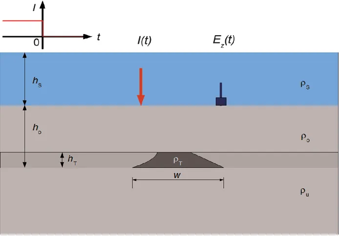
Figure 6. Schematic presentation of the acquisition system based on current injection using a vertical bipole and

registration of the vertical component of the electric field. The injected current is switched off at t ¼ 0. Parameters hS, ho, hT indicate the water depth, the overburden, and reservoir thicknesses; ρS, ρo, ρu, ρT are the water, overburden, underburden, and reservoir resistivities; w specifies the horizontal extent of the reservoir. The case of w ¼ 0 corresponds to a stratified structure without a reservoir; the case of w ¼ ∞ corresponds to a stratified structure with the reservoir unlimited in both horizontal directions

A VED source does not create the TE-mode in a stratified medium, so that equations governs to

(29)

20

𝑗 = 𝜎_𝑏𝐸 = −∇_𝜏𝜕_𝑧𝑊 + 𝑒_𝑧∇_𝑧2_𝑊

𝐻 = 𝑒_𝑧 × ∇_𝜏𝑊

The field is sensitive to relatively resistive layers. Compared to the traditional SBL approach, the measured signal is weaker, but it is usually preferable to directly measure small signals associated with the surveyed target, rather than to extract corresponding data from stronger signals contaminated by an unrelated to the target information. In particular, the VED source does not create an air-wave that dominates the SBL responses at large offsets (Bension Sh. Et. Al., 2013).

The vertical electric field is sensitive to deep resistive layers at late times the vertical electric field decays like 𝐸𝑧(𝑡) ≈ 𝑡−5 2⁄ over a rock of uniform conductivity. Using a vertical dipole and vertical receiver for marine borehole measurements has been suggested by Scholl and Edwards (2007).

Vertical transmitter (Figure 7.), is sensitive to horizontal resistive layers, and therefore carries information about the deeper structures. The upper electrode is kept at a fixed distance of 30-50m below sea surface independent of depth, to keep track of its position, and to utilize the maximum possible transmitter dipole length (Terje Holten et. al. 2009). The magnitude of the external electromagnetic noise decreases with depth, because of the skin depth effect that dampens high frequencies. Hence, the signal-to-noise ratio usually increases with water depth. The advantage with time-domain measurements, is that there is no need for separation of the low amplitude signal from the deep layers from the noise resulting from the movement of the upper electrode. There is no air-wave because of the vertical transmitter, and the reduced signal level is the limiting factor for shallow water surveys.

The challenge when measuring the vertical, rather than the horizontal field, is the small amplitude of the signal. At late times the horizontal response from a horizontal dipole is 2−3 orders of magnitude stronger than the vertical response from a vertical dipole (Chave and Cox, 1982).

The optimal offset can be found, which is usually in the range from 500 m −1500 m. The response from the underground is recorded while the transmitter is off, so that the uncertainties of the location of the pulse electrodes do not lead to a time dependent noise. Verticality eliminates the air-wave components from the received signal.

(30)

21

Figure 7. An overview of the Petromarker technology (not to scale), only one pulse system is shown. The upper and lower pulse electrodes which are directly on top of each other form the vertical transmitter dipole, the return current goes through the sea. To the left on the sea bottom, the extensible tripod is shown, and to the right, a flexible cable receiver. The colour scale (unit log10 (|Ez| (in V/m)) of the sediments represents the vertical electric field in the presence of the HC-filled reservoir (yellow). The electric field is evaluated for a 5000 Am source dipole shortly before the current is turned off.

1.4.5.1.3 Towed source EM (TSEM)

The current generation of the towed-streamer EM system consists of an electric Dipole source towed at a depth of 10 m below the sea surface, and up to a 9-km-long streamer of the electric field receivers towed at a depth of approximately 100 m. Figure 8 presents the corresponding layout of the towed-streamer EM system (Anderson, C., and J. Mattsson, 2010). The injected electric current from the source is transmitted as optimized repeated sequences (ORS), in which each sequence consists of a 100-s-long active part (source on) followed by a 20 s silent period (source off). The source sequence is designed to obtain as high energy as possible in a discrete set of frequencies, in which the electric field response is sensitive to the resistive anomaly. Mattsson et al. (2012) describe the deconvolution and current noise reduction methodology for the towed-streamer EM system.

(31)

22

Figure 8. A sketch of the towed-streamer EM system.

The towed-streamer EM system makes it possible to collect EM data with a high production rate and over very large survey areas. At the same time, 3D inversion of the towed-streamer EM data is a very challenging problem because of the huge number of transmitter positions of the moving towed-streamer EM system, and, correspondingly, the huge number of the forward and inverse problems needed to be solved for every transmitter position over the large areas of the survey (Ramananjaona, et. Al., 2011).

The prototype system described here is sufficiently powerful to work in water depths up to 400 m, with a nominal depth penetration of 2,000 m below the seafloor. The signal is a transient signal that can be a modified square-wave, or a PRBS (Folke Engelmark, et. Al., 2012).

Towed EM, as described by Anderson and Mattsson (2010), has numerous advantages:

 Improved efficiency: source and receiver towed from the same vessel.

 Operationally similar to marine seismic.

 Real time monitoring and QC of source and receiver cable.

 On-board pre-processing.

 Dense sub-surface sampling.

 Receivers towed above the seafloor. The influence of strong local anomalies at the seabed is minimized.

 Facilitates simultaneous acquisition of EM and 2D seismic.

The reason towed EM has not been available until now is that the relative movement between the receiver sensors and the seawater generate a voltage that is typically much

(32)

23

larger than the signal voltage. This was a crucial issue that had to be resolved before bringing the system to the market.

To characterize sensitivity of the CSEM method to the given target, we use the following quantity:

𝑆 = |𝐸𝑇𝐴 − 𝐸𝐵𝐺| 𝛼|𝐸_𝐵𝐺| + 𝜂

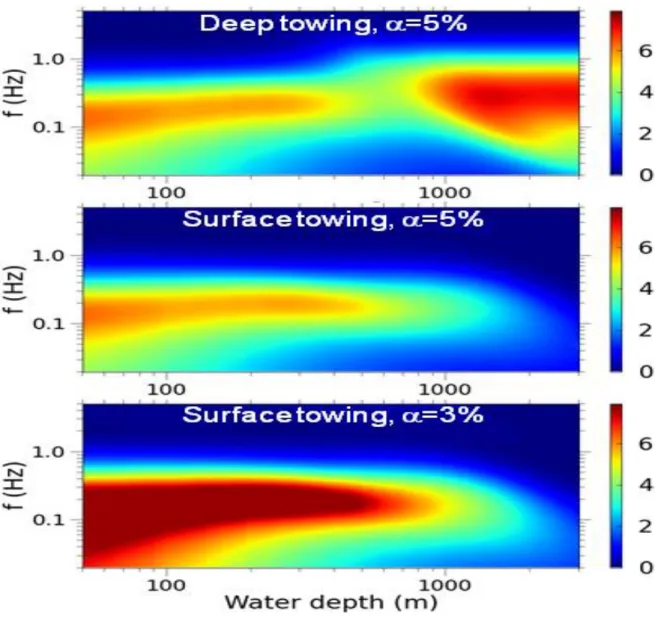
The numerator represents the absolute value of the scattered field, i.e. the difference between the field in the presence of target ETA and the background field EBG, First, the sensitivity is computed as a function of the source receiver offset for a given frequency f and water depth(D.V. Shantsev, F. Roth and H. Ramsfjell, 2012).

The advantage of the deep towing is that very little EM energy is lost while propagating through the sea water, therefore it is preferred at larger water depths. We however demonstrate that in water depths of 250 m or less surface towing is likely to become the standard operation. At these depths, surface towing gives equally good results in terms of sensitivity and inversion as deep towing, while at the same time allowing a superior operational efficiency. The exact water depth threshold will depend on the specific target depth and geologic setting, and must be established through modeling and inversion during survey planning (D.V. Shantsev, F. Roth and H. Ramsfjell, 2012).

The relative uncertainty for a typical CSEM survey can be taken as 5% (Zach et al., 2009). The second term is the noise floor, which is determined by magneto-telluric noise, sensor noise, swell noise, etc. It is set to h = 10−15V/Am2 (after scaling by the source dipole moment).

First, the sensitivity is computed as a function of the source receiver offset for a given frequency f and water depth. Then we select its maximal value over all offsets and plot it as a map in the plane (f – water depth) in Figure 9.

(33)

24

Figure 9. Sensitivity maps of the CSEM method for deep towing (top) and surface towing for a = 5% (middle) and a = 3%

(bottom). The sensitivity is defined as the target response normalized to uncertainty, Eq. 1. The surface towing provides equal or better sensitivity if the water depth is smaller than 450 m. Reduction in the navigation uncertainty (a = 3%) moves the threshold depth to 700 m. Target depth is 2 km.

Obviating the need for ocean bottom receivers, the towed EM system enables CSEM data to be acquired simultaneously with seismic over very large areas in frontier and mature basins for higher production rates and relatively lower cost than conventional CSEM methods. The increased volume of CSEM data represents a challenge to existing 3D CSEM inversion methods.

1.4.5.2 CSEM Survey

Electromagnetic fields are useful in geophysics due to their interactive nature with the medium through which they propagate (Zhdanov 2009). This interaction can be used to

(34)

25

determine certain physical properties of rocks, these being electrical conductivity σ, dielectric permittivity ε, and magneticpermeability μ. The electromagnetic methods are based on the study of the propagation of electric currents and/or electromagnetic fields in the Earth.

Electrical resistivity of the subsurface provides important information on the porosity and pore geometry of the geologic formations as well as the nature of the fluids that fill the pore spaces. Resistivity increases exponentially for hydrocarbon bearing rocks, resulting into a strong resistivity contrast between gas-saturated and brine-saturated geological media. Until of recent, the seismic method has been the dominant technique used for reservoir detection and monitoring. Due to its shortcomings, different electromagnetic methods have been developed to detect and monitor geological hydrocarbons. Electromagnetic (EM) methods have provided a more cost effective monitoring technique that, at a minimum, has reduced the frequency of seismic surveys. CSEM which exploits the conductivity contrasts in the subsurface sediments has become an important complementary tool for offshore petroleum exploration prior to drilling (Eidesmo, S. Ellingsrud et al. 2002, Mehta.K, Nabighian.M et al. 2005, Bakr and Mannseth 2009). Marine CSEM survey has been used in; estimating the formation resistivity without using borehole logs (Constable and Weiss 2006), CO2 sequestration monitoring (Kang, Seol et al. 2011), and 3D modeling and time-lapse of CO2 (Bhuyian, Landrø et al. 2012). It can effectively detect marine reservoirs with high saturation of up to 60- 80% (Wang, Luo et al. 2008, Constable 2010). This technique has been used mainly in discriminating between the hydrocarbon and the water-filled rocks in addition to estimating the geometry of the hydrocarbon (Bhuyian, Landrø et al. 2012). Hydrocarbons have a low conductivity less than 0.01 S/m while the formation water has a high conductivity of up to 10 S/m. Hence, the EM signal is strongly influenced by the porefluid contents (Bhuyian, Landrø et al. 2012).

1.4.5.2.1 Forward Modeling

Modeling data plays an important role in the standardization of the background field and the reservoir dimensions that play an important role during time-lapse CSEM monitoring. Time lapse CSEM can normally be used as a reservoir monitoring tool to help in the reservoir management (Bhuyian, Landrø et al. 2012). Assuming that other changes in the reservoir properties remain unaffected by the changes in the pore-fluid content, monitoring the production of hydrocarbons will help to observe and track any changes in the subsurface distribution through detection of changes in conductivity. The developed methods were tested for monitoring of geolectrical data to model the changes in saturation as reservoir production took place.

(35)

26 1.4.5.2.2 Inverse Modeling

Inversion of marine CSEM data has been previously done using Bayesian algorithm (Ray and Key 2012). Torres-Verdin and Habashy (1995) performed a linear inversion of 2D electrical conductivity. Basing on these studies, 3D inversion modeling of CSEM data has been done. In solving the inverse problems, the mathematical difficulty is that the inverse operator may not exist or may not be continuous over a given domain. Electromagnetic inversion methods are widely used in the interpretation of geophysical electromagnetic data in mineral, hydrocarbon, and underground water exploration. The EM response of the petroleum reservoir is weak compared to the background EM field generated by an electric dipole transmitter in layered geoelectric structures (Zhdanov 2009) ; thus rendering inversion of CSEM data a problem.

Bhuyian, Landrø et al. (2012) and Shahin, Key et al. (2010) noted that time-lapse CSEM data is achieved by carrying out several repeated surveys over a depleting reservoir at different times with the major aim of detecting and estimating the changes in the pore filling fluid properties. The main aim of CSEM monitoring is to image fluid flow in a reservoir during production since the electrical properties do change with fluid saturation. The monitoring process unlike exploration, is easily carried out and normally inexpensive since; (1) the same equipment used in the exploration are also used during the monitoring; (2) knowledge about the reservoir location and conductivity is acquired prior to monitoring; (3) the receivers being anchored on the seafloor reduces the experimental errors which would otherwise affect the process after subsequent surveys and ensures maximum mapping of the same target. According to Lien and Mannseth (2008), monitoring helps in determining the sensitivity of the CSEM data with respect to changes in conductivity distributions. For enhanced oil production, brine or gas is injected into the depleted reservoir to displace the remaining oil towards the production well. Here, the main focus will be the detection of the electrical conductivity changes for a horizontal flooding with a two-phase zone separating the saline water and the saturated sediments; thus the reservoir being heterogeneous with varying brine saturations. As more conductive brine is injected into a depleted reservoir, conductivity increases there by decreasing the contrast. A decrease in conductivity contrast of the reservoir decreases the electric field indicating the change in the saturation of the hydrocarbon. Therefore, it will be expected that as more brine is injected, the formation resistivity of the reservoir increases. The extent to which the brine has migrated into the reservoir will be detected by the change in the anomalous electric field.

(36)

27

Inversion or “inverse modeling” attempts to reconstruct subsurface features from a given set of geophysical measurements, and to do so in a manner that the model response fits the observations (Treite, et al., 1999).

Figure 10. Schematic representation of inverse modeling (Snieder, et al., 1999)

1.4.5.3 Noise of System

The noise on the transmitter/receiver system represents an evident role in survey design. The CSEM noise is categorized as systematic and non-systematic noise. The first includes instruments noise and positioning error, further, its value is normally assumed to be proportional to the amplitude of the CSEM signal. The latter instead is independent of the signal, Kwon (2003) indicates a noise value of electric field equal to 0.5 V/m. The systematic noise decreases with the frequency since the amplitude of the signal tend to decreases increasing the frequency. We deduce that, for the lowest CSEM frequencies, from 0.1 to 2Hz, the systematic noise is predominant. Constable and Weiss (2006) has also derived the typical noise floor value due to the systematic noise component. For a receiver voltage noise Vr measured in V/m, a bandwidth B, and a source dipole moment SDM measured in A · m the electric-field noise is given by

𝐸_𝑛 = 𝑉𝑟

𝑒(𝑆𝐷𝑀)√𝐵

As example, for instruments having a voltage noise of 10−9V √Hz at 1 Hz and a source dipole moment of 450 KAm we get an electric-field noise of 2 · 10−15 V/Am2. Such value is assumed as the reference noise floor for CSEM systems. Data for interpretation are normalized by the dipole moment, so the system noise floor gets lower as SDM gets larger, allowing larger source-receiver offsets to be recorded and deeper structure to be detected. About the magnetic field, in literature (Constable, 2010) is indicated the reference value 10−18 1/m3 as noise floor (magnetic field normalized to the SDM).

(37)

28 1.4.5.3.1 Air Wave Effect

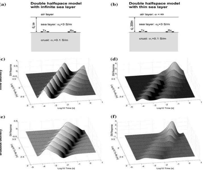
Of particular concern to companies who explore in shallow waters such as the shelf seas is the so called air wave. Some portion of the electromagnetic energy travels upwards to the sea surface, through the air to the vicinity of the receiver and then downwards to the receiver on the sea floor. The up over- down path can in some instances be faster than any direct path through the sea water or the subjacent crust. Compare the two models shown in Figure 11a, b and the stacked impulse response of these models shown in Figure 11c–f, for the in-line and broadside geometries. The sea layer in the first model is infinitely thick while that in the second has a finite thickness of 200 m. As the transmitter–receiver separation increases, the air wave which initially appears at later time appears to move to relatively earlier times and at large separations contaminates the disturbance travelling through the crust. From a practical point of view, the air wave signature is easily removed in the inversion of data provided sufficient dynamic range in the receiver electronics is available to record it properly (Edwards, 2005).

(38)

29

Figure 11. The airwave. The normalized impulse responses of the models in (a) and (b) to an electric dipole–dipole system on the seafloor are shown as functions of logarithmic time and transmitter receiver separation. Panels (c) and (d) refer to inline and panels (e) and (f) to broadside geometries.

(39)

30