MODEL CHECKING SPATIAL LOGICS FOR CLOSURE SPACES∗ VINCENZO CIANCIAa, DIEGO LATELLAb, MICHELE LORETIc, AND MIEKE MASSINKd
a,b,dIstituto di Scienza e Tecnologie dell’Informazione “A. Faedo” - CNR, Pisa
e-mail address: {vincenzo.ciancia, diego.latella, mieke.massink}@isti.cnr.it
c
Universit`a degli Studi di Firenze and IMT Alti Studi, Lucca e-mail address: [email protected]
Abstract. Spatial aspects of computation are becoming increasingly relevant in Computer Science, especially in the field of collective adaptive systems and when dealing with systems distributed in physical space. Traditional formal verification techniques are well suited to analyse the temporal evolution of programs; however, properties of space are typically not taken into account explicitly. We present a topology-based approach to formal verification of spatial properties depending upon physical space. We define an appropriate logic, stemming from the tradition of topological interpretations of modal logics, dating back to earlier logicians such as Tarski, where modalities describe neighbourhood. We lift the topological definitions to the more general setting of closure spaces, also encompassing discrete, graph-based structures. We extend the framework with a spatial surrounded operator, a propagation operator and with some collective operators. The latter are interpreted over arbitrary sets of points instead of individual points in space. We define efficient model checking procedures, both for the individual and the collective spatial fragments of the logic and provide a proof-of-concept tool.
1. Introduction
Much attention has been devoted in Computer Science to formal verification of process behaviour. Several techniques have been studied and developed that are based on a formal understanding of system requirements through modal logics. Such logics typically have a temporal flavour, describing the flow of events, and are interpreted in various kinds of transition structures. Among those techniques model checking is one of the most successful (for an extensive overview see e.g. [BK08] and references therein).
In recent times, aspects of computation related to the distribution of systems in physical space have become increasingly relevant. An example is provided by so called collective adaptive systems1. Such systems are typically composed of a large number of interacting
2012 ACM CCS: [Theory of computation]: Logic—Logic and verification / Modal and temporal logics / Verification by model checking; Semantics and reasoning; [Software and its engineering]: Software organization and properties—Software functional properties—Formal methods—Software verification;
Key words and phrases: Spatial Logics, Spatial Model Checking, Closure Spaces, Collective Logics.
∗
Research partially funded by EU project QUANTICOL (nr. 600708).
1See e.g. the web site of the QUANTICOL project: http://www.quanticol.eu, and that of the FOCAS
Coordination Action: http://www.focas.eu.
LOGICAL METHODS
l
IN COMPUTER SCIENCE DOI:10.2168/LMCS-12(4:2)2016c
V. Ciancia, D. Latella, M. Loreti, and M. Massink CC
objects located in space. Their global behaviour critically depends on interactions which are often local in nature. The aspect of locality immediately poses issues of spatial distribution of objects. Abstraction from spatial distribution may sometimes provide insights in the system behaviour, but this is not always the case. For example, consider a bike (or car) sharing system having several parking stations, and featuring twice as many parking slots as there are vehicles in the system. Ignoring the spatial dimension, on average, the probability to find completely full or empty parking stations at an arbitrary station is very low; however, this kind of analysis may be misleading, as in practice some stations are much more popular than others, often depending on nearby points of interest. This leads to quite different probabilities to find stations completely full or empty, depending on the examined location. In other cases, it may be important to be able to specify spatial properties concerning groups of points in space rather than of individual points. For example, the property that agents associated to points in space are able to connect to one another and act as a group, or that they are located all together in a protected environment, or that they can share part of the same route to reach a common exit or goal. In all such situations, it is important to be able to predicate over spatial aspects, and eventually find methods to certify that a given collective adaptive system satisfies specific requirements in this respect.
In Logics, there is a considerable amount of literature focused on so called spatial logics, that is, a spatial interpretation of modal logics [APHvB07]. Dating back to early logicians such as Tarski, modalities may be interpreted using the concept of neighbourhood in a topological space. The field of spatial logics is well developed in terms of descriptive languages and decidability or complexity aspects. However, in this field, scant attention has been devoted to date to the development of formal and automatic verification methods, e.g. model checking. Furthermore, the formal treatment of discrete models of space is still a relatively unexplored field, with notable exceptions such as the work by Rosenfeld [KR89, Ros79], Galton (e.g.[Gal14, Gal03, Gal99]) and by Smyth and Webster [SW07]. Kovalevsky [Kov08] studied alternative axioms for topological spaces in order to recover well-behaved notions of neighbourhood. The outcome is that one may impose closure operators on top of a topology, that do not coincide with topological closure.
In [CLLM14a] we proposed the logic SLCS (Spatial Logic for Closure Spaces), extending the topological semantics of modal logics to closure spaces. The work follows up on the research line of Galton and Smyth and Webster, enhancing it with a modal logic perspective. Closure spaces (also called ˇCech closure spaces or preclosure spaces in the literature) are based on a single operator on sets of points, namely the closure operator, and are a generalisation of standard topological spaces. In addition, finite spaces and graphs are subclasses of closure spaces and the graph-theoretical notion of neighbourhood coincides with the notion of neighbourhood defined in the context of closure spaces. Thus, closure spaces provide a uniform framework for the treatment of all major models of space.
We provided a logical operator corresponding to the closure operator on sets of points in space, and a spatial interpretation of the temporal until operator, fundamental in the classical temporal setting, arriving at the definition of a logic which is able to describe unbounded areas of space. Intuitively, the spatial until operator, which in the present paper we call surrounded, describes a situation in which it is not possible to “escape” an area of points satisfying a certain property, unless by passing through at least one point that satisfies another given formula. This operator is similar in spirit to the spatial until operator for topological spaces discussed by Aiello and van Benthem in [Aie02, BB07]. In [CLLM14a] we also presented a model-checking algorithm for SLCS when interpreted on finite models.
The combination of SLCS with temporal operators from the well-known branching time logic CTL (Computation Tree Logic) [CE82], has been explored in [CGL+15, CLMP15] and provides spatio-temporal reasoning and model checking.
In the present paper we extend SLCS with a further operator, P, capturing the notion of spatial propagation; intuitively the formula φ P ψ describes a situation in which the points satisfying ψ can be reached by paths rooted in points satisfying φ and, for the rest, composed only of points satisfying ψ. We furthermore extend the logic with operators for collective properties, namely properties which are satisfied by connected sets of points, rather than points in isolation. The formal semantics of the extended logic—CSLCS, Collective SLCS–are provided in the form of a satisfiability relation defined using the notion of infinite path in closure spaces. We finally extend the model-checking algorithm in order to treat the newly introduced operators, and we present several examples of use of SLCS and CSLCS from the domain of collective adaptive systems using a prototype implementation of the spatial model-checker.
Related work. Variants of spatial logics have also been proposed for the symbolic rep-resentation of the contents of images, and, combined with temporal logics, for sequences of images [DBVZ95]. The latter approach is based on a discretisation of the space of the images in rectangular regions and the orthogonal projection of objects and regions onto Cartesian coordinate axes such that their possible intersections can be analysed from different perspectives. It involves two spatial until operators defined on such projections considering spatial shifts of regions along the positive, respectively negative, direction of the coordinate axes and it is very different from the topological spatial logic approach.
In [GBC+08, GSC+09, GBB14] another variant of spatial logic is proposed in which spatial properties are expressed using ideas from image processing, namely quad trees. This variant is equipped with practical model checking algorithms and with machine learning procedures and allows one to capture very complex spatial structures. However, this comes at the price of a complex formulation of spatial properties, which need to be learned from some template image. The combination of this spatial logic with linear time signal temporal logic, defined with respect to continuous-valued signals, has recently led to the spatio-temporal logic SpaTeL [HJK+15].
In the specific setting of complex and collective adaptive systems, techniques for efficient approximation have been developed in the form of mean-field or fluid-flow analysis (see [BHLM13] for a tutorial introduction). Recently (see for example [CLBR09]), the importance of spatial aspects has been recognised and studied in this context. In [NB14] a first step towards the combination of signal temporal logic with spatial operators such as ‘somewhere’ and ‘everywhere’ has been performed. These two operators were also proposed in work by Reif and Sistla [RS85]. In further joint work along these lines [NBC+15] some of the spatial operators based on closure spaces from SLCS, such as the ‘surrounded’ operator, have been added to the signal temporal logic fraction. Both boolean semantics and quantitative semantics of the spatio-temporal logic have been provided. The quantitative semantics provide a measure of the robustness with which a spatio-temporal property holds in a given point in space at a particular time. The approach has been applied to investigate the emergence and persistence of Turing patterns in animal fur based on reaction diffusion models.
In [CG12] a geometric process algebra based on affine geometry has been proposed for describing the concurrent evolution of geometric structures in 3D space. Spatial dynamics of
systems have also been studied in the context of Systems Biology applying suitable modelling and simulation approaches. In [JEU08] a spatial (and temporal) extension of the π-Calculus is proposed. The notion of space is expressed by associating each process with its current position in Rd. The formal semantics of the language is given, based on which simulation
tools have been developed. In [BHMU11] an attributed, multi-level, rule-based language, ML-Space, is presented that allows one to integrate different types of spatial dynamics within one model. The associated simulator combines several stochastic simulation methods. This allows for the simulation of reaction diffusion systems as well as taking excluded volume effects into account. Formal verification and analysis, e.g. model checking, is not addressed.
In the Computer Science literature, some spatial logics have been proposed, that typically describe situations in which modal operators are interpreted syntactically against the structure of agents in a process calculus. We refer to [CG00, CC03] for some classical examples. In the same line, a recent example is given by [TPGN15], concerning model checking of security aspects in cyber-physical systems, in a spatial context based on the idea of bigraphical reactive systems introduced by Milner [Mil09]. The objects of discussion in the latter research lines are operators that for example quantify over the parallel sub-components of a system, the containment relation between places, or the hidden resources of an agent. The meaning of the terminology “spatial logics” in that case is different from that used in the present paper, where the “topological” interpretation of [BB07] is intended. The influence of space on agents interaction is also considered in the literature on process calculi using named locations [DFP98], where every process interaction primitive is enriched with the indication of (the name of) the location where the action operates. In that paper, space is modelled as a discrete, finite set of points.
Logics for graphs have been studied in the context of databases and process calculi (see [CGG02, GL07], and the references therein), even though the relationship with physical space is often only implicit, if considered at all.
Graph-based spatial logics for collective adaptive systems are also proposed in [AS15]. In that approach the logic extends a chemical-based coordination model based on logic inference. Properties are expressed in the form of combinations of logic programs. The spatial operators distribute such programs over the nodes of a graph to infer information local to each node. The locally inferred data is logically aggregated at local spatial locations. Evaluated properties involve collective aspects either with a local scope (neighbourhood) or with a global scope. The approach relies on a priori defined spatial patterns.
A successful attempt to bring topology and digital imaging together is represented by the field of digital topology [Ros79, KR89]. In spite of its name, this area studies digital images using models inspired by topological spaces, but neither generalising nor specialising these structures. Rather recently, closure spaces have been proposed as an alternative foundation of digital imaging by various authors, especially Smyth and Webster [SW07] and Galton [Gal03]; we continue that research line in the present paper, enhancing it with a (modal) logic perspective.
In [Gal14], a sub-class of closure spaces, namely adjacency spaces, is presented. An adjacency space is characterized by a set of entities together with a reflexive and symmetric relation. In the above mentioned paper, adjacency spaces are used as the basis for the definition of regions, i.e. sets of entities, and the construction of a discrete interpretation of logical operators typical of region calculi, based on the notion of region connectedness derived from the notion of entity adjacency. Region calculi operators predicate on regions (see [KKWZ07] for a comprehensive overview), using boolean connectives like “part of”,
“boundary”, “overlap” and so on. An important aspect of adjacency spaces is that they can be easily turned into topological spaces, without loosing any information on their internal structure, which makes them rather attractive. Verification issues, e.g. model-checking, are not addressed in [Gal14].
The structure of the present paper is as follows. Section 2 recalls basic concepts and definitions related to closure spaces, their sub-classes of topological spaces and quasi-discrete closure spaces and introduces the notion of Euclidean and quasi-discrete paths in closure spaces. Section 3 briefly recalls SLCS and presents its extension with the propagation operator P. Section 4 introduces the collective spatial logic CSLCS while Section 5 shows some examples of use of the proposed logics when interpreted on quasi-discrete closure spaces. In Section 6 the model-checking algorithms for SLCS and CSLCS interpreted on finite models are presented. In Section 7 the proof-of-concept model-checker is shown together with several examples of use. Finally, some conclusions are drawn and lines for future research are outlined in Section 8. All detailed proofs are provided in the Appendix.
2. Topological and Closure spaces
In this work, we resort to some abstract mathematical structures for the definition of space. The mathematical structure of choice of spatial logics are very often topological spaces, possibly enriched with metrics, or other spatial features (see [BB07]). The use of abstract structures has the advantage to separate logical operators, such as neighbourhood, from the specific nature of space (e.g., the number of dimensions, or the presence or absence of metric features, etc.). However, using topological spaces, it may be difficult to deal with discrete structures, such as finite graphs. In [Gal03], closure spaces, which generalise topological spaces, are proposed as a unifying approach treating both topological spaces and graphs in a satisfactory way. In this section, we recall several definitions and results on topological and closure spaces, most of which are taken from [Gal03].
2.1. Topological spaces. We will first provide the basic definitions that are used to relate closure spaces to the more widely known topological spaces. The link between topological and closure spaces is deep. In this section we provide a brief introduction to the topic; we refer the reader to, e.g., [Gal03] for more information.
Definition 2.1. A topological space is a pair (X, O) of a set X and a collection O ⊆ ℘(X) of subsets of X called open sets, such that ∅, X ∈ O, and subject to closure under arbitrary unions and finite intersections.
Definition 2.2. In a topological space (X, O), A ⊆ X is closed if its complement is open. Definition 2.3. In a topological space (X, O), the closure of A ⊆ X is the least closed set containing A.
We remark that closure is well-defined as arbitrary intersections of closed sets are closed, and X itself is both open and closed. An alternative, equivalent formulation of topological spaces is given by the Kuratowski definition.
Definition 2.4. According to the Kuratowski definition, a topological space is a pair (X, C) where X is a set, and the closure operator C : ℘(X) → ℘(X) assigns to each subset of X its closure, obeying to the following laws, for all A, B ⊆ X:
(1) C(∅) = ∅; (2) A ⊆ C(A);
(3) C(A ∪ B) = C(A) ∪ C(B); (4) C(C(A)) = C(A).
The Kuratowski and open sets definitions of a topological space are equivalent. The proof can be sketched as follows. To obtain the Kuratowski definition from a topological space defined in terms of open sets, one defines C(A) as topological closure (Definition 2.3). The properties of Definition 2.4 can be shown to hold. For the converse, starting from a Kuratowski topological space (X, C), the open sets are defined as those sets A that are equal to their interior, that is, A = C(A) where for any B ⊆ X we let B denote the complement of B, i.e. X \ B.
2.2. Closure spaces. A closure space (also called ˇCech closure space or preclosure space in the literature), is composed of a set (of points) and a (closure) operator on subsets (of points), as specified by the following definition:
Definition 2.5. A closure space is a pair (X, C) where X is a set, and the closure operator C : ℘(X) → ℘(X) assigns to each subset of X its closure, obeying to the following laws, for all A, B ⊆ X:
(1) C(∅) = ∅; (2) A ⊆ C(A);
(3) C(A ∪ B) = C(A) ∪ C(B).
Closure spaces are a generalisation of topological spaces, which is easy to see by comparing Definition 2.5 with Definition 2.4; the difference is that the idempotency axiom C(C(A)) = C(A) is not required in closure spaces. Indeed, topological spaces are precisely the subclass of closure spaces where such axiom holds. We shall call a closure space topological or idempotent or Kuratowski in that case. We note in passing that the notion of continuous function also extends to closure spaces (see Definition 2.30), making closure spaces a category in the sense of category theory, and topological spaces a full subcategory.
Below, we consider an example of a closure space, with set of points X in a classical Euclidean space, but exhibiting a non-standard closure operator.
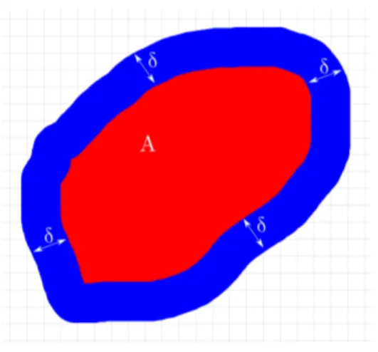
Example 2.6. Let δ ∈ R>0 and Cδ : ℘(R2) → ℘(R2) be such that:
Cδ(A) = {(x1, y1) ∈ R2|∃(x2, y2) ∈ A.
p
(x2− x1)2+ (y2− y1)2 ≤ δ}
Function Cδ maps each subset A of R2 to the set of points located in a radius δ from a point
in A (see Figure 1). It is easy to see that Cδ satisfies all the three conditions of Definition 2.5
and that (R2, Cδ) is a closure space.
Example 2.7. The closure space of Example 2.6 is not a topological space, as its closure operator is not idempotent.
Definition 2.8. Let (X, C) be a closure space; for each A ⊆ X: (1) the interior I(A) of A is the set C(A);
(2) A is a neighbourhood of x ∈ X if and only if x ∈ I(A); (3) A is closed if A = C(A) while it is open if A = I(A).
Figure 1: A picture of Example 2.6; the union of the blue and red areas is the closure of the red area
Example 2.9. Let us consider the closure space (R2, Cδ), introduced in Example 2.6,
assuming, for simplicity, that δ ≤ 1. Let A = {(x, y) ∈ R2|px2+ y2 ≤ 1}. We have that:
• I(A) = {(x, y) ∈ R2|p
x2+ y2≤ 1 − δ};
• for any (x1, y1) ∈ R2, A is a neighbourhood of (x1, y1) if and only if:
{(x2, y2) ∈ R2|
p
(x2− x1)2+ (y2− y1)2 ≤ δ} ⊆ A
• the only closed set (of the closure operator Cδ) in ℘(R2) is R2, while ∅ is the only open set.
The following proposition states a number of general properties of closure spaces. Proposition 2.10. Let (X, C) be a closure space, the following properties hold: (1) A ⊆ X is open if and only if A is closed;
(2) closure and interior are monotone operators over the inclusion order, that is: A ⊆ B =⇒ C(A) ⊆ C(B) and I(A) ⊆ I(B)
(3) Finite intersections and arbitrary unions of open sets are open.
Given a closure space (X, C), and A ⊆ X, we can define the boundary of A. The latter is only given in terms of closure and interior, and coincides with the definition of boundary in a topological space. We also provide two similar notions, namely the interior and closure boundary (the latter is sometimes called frontier ).
Definition 2.11. In a closure space (X, C), the boundary of A ⊆ X is defined as B(A) = C(A) \ I(A). The interior boundary is B−(A) = A \ I(A), and the closure boundary is
B+(A) = C(A) \ A.
In [Gal99], a discrete variant of the topological definition of the boundary of a set A is given, for the case where a closure operator is derived from a reflexive and symmetric relation (see Definition 2.16 in the next section). Therein, in Lemma 5, it is proved that the definition of [Gal99] coincides with the one we provide above.
Proposition 2.12. The following equations hold in a closure space:
B(A) = B+(A) ∪ B−(A) (2.1)
B+(A) ∩ B−(A) = ∅ (2.2)
B(A) = B(A) (2.3)
B+(A) = B−(A) (2.4)
B+(A) = B(A) ∩ A (2.5)
B−(A) = B(A) ∩ A (2.6)
B(A) = C(A) ∩ C(A) (2.7)
A closure space can be also obtained by restricting the domain of another space. Definition 2.13. Given a closure space (X, C) and a subset Y ⊆ X, we call subspace closure the operation CY : ℘(Y ) → ℘(Y ) defined as CY(A) = C(A) ∩ Y . We call (Y, CY) the subspace of (X, C) generated by Y .
Proposition 2.14. The subspace closure is a closure operator. Example 2.15. (R2≥0, C
R2≥0
δ ) is a subspace of the closure space (R2, Cδ) introduced in
Example 2.6, generated by R2 ≥0.
2.3. Quasi-discrete closure spaces. A closure space may be derived starting from a binary relation, that is, a graph. Such closure spaces may be characterised as quasi-discrete as briefly presented in this section. For additional details we refer the interested reader to [Gal03].
Definition 2.16. Consider a set X and a relation R ⊆ X × X. A closure operator is obtained from R as CR(A) = A ∪ {x ∈ X | ∃a ∈ A.(a, x) ∈ R}.
Proposition 2.17. The pair (X, CR) is a closure space.
Closure operators obtained by Definition 2.16 are not necessarily idempotent. Lemma 11 in [Gal03] provides a necessary and sufficient condition, that we rephrase below. We let R= denote the reflexive closure of R, that is, the smallest reflexive relation containing R, which is defined as the union of R with the identity relation on the same domain.
Lemma 2.18. CR is idempotent if and only if R= is transitive.
Note that when R is transitive, so is R=, thus C
R is idempotent. The vice-versa is not
true. For instance, it may happen that (x, y) ∈ R, and (y, x) ∈ R, but (x, x) /∈ R.
Remark 2.19. In topology, open sets play a fundamental role. However, the situation is different in closure spaces derived from a relation R. For example, in a closure space derived from a symmetric relation, whose graph is connected, the only open sets are the whole space, and the empty set.
Proposition 2.20. Given R ⊆ X × X, in the space (X, CR), we have:
I(A) = {x ∈ A | ¬∃a ∈ A.(a, x) ∈ R} (2.8)
B−(A) = {x ∈ A | ∃a ∈ A.(a, x) ∈ R} (2.9)
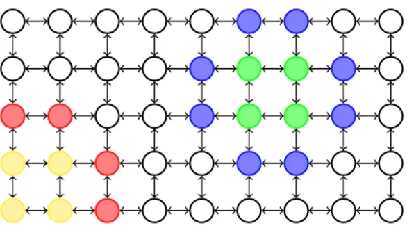
Figure 2: A graph inducing a quasi-discrete closure space
Closure spaces derived from a relation can be characterised as quasi-discrete spaces (see also Lemma 9 of [Gal03] and the subsequent statements).
Definition 2.21. A closure space is quasi-discrete if and only if one of the following equivalent conditions holds:
i) each x ∈ X has a minimal neighbourhood2 Nx;
ii) for each A ⊆ X, C(A) =S
a∈AC({a}).
The following is proved as Theorem 1 in [Gal03].
Theorem 2.22. A closure space (X, C) is quasi-discrete if and only if there is a relation R ⊆ X × X such that C = CR.
Summing up, whenever one starts from an arbitrary relation R ⊆ X × X, the obtained closure space (X, CR) enjoys minimal neighbourhoods, and the closure of a set A is the union
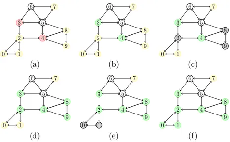
of the closure of the singletons composing A. Furthermore, such nice properties are only true in a closure space when there is some R such that the closure operator of the space is derived from R. In the remainder of this section, we exemplify some aspects of quasi-discreteness. Example 2.23. Every graph induces a quasi-discrete closure space. For instance, consider the (undirected) graph depicted in Figure 2. Let R be the (symmetric) binary relation induced by the graph edges, and let Y and G denote the set of yellow and green nodes, respectively. The closure CR(Y ) consists of all yellow nodes and red nodes, while the closure
CR(G) contains all green nodes and blue nodes. The interior I(Y ) of Y contains a single
node, the one located at the bottom-left in Figure 2. The interior I(G) of G is empty. Indeed, we have that B(G) = CR(G), while B−(G) = G and B+(G) consists of the blue
nodes.
Example 2.24. The closure space of Example 2.6 is a quasi discrete closure space. Indeed, define Rδ⊆ R2× R2 as:
Rδ = {((x1, y1), (x2, y2))|
p
(x2− x1)2+ (y2− y1)2 ≤ δ}
It is easy to prove that Cδ= CRδ. Note that Rδ is reflexive but not transitive. So, the closure space is not a topological space.
Existence of minimal neighbourhoods does not depend on finiteness of the space; moreover, it is not even required that each point has a finite neighbourhood, as illustrated by the following example:
2A minimal neighbourhood of x is a set that is a neighbourhood of x (Definition 2.8 (2)) and is included
Figure 3: A quasi-discrete closure space inducing a spatial structure.
Example 2.25. Consider the rational numbers Q, with the relation ≤. Such a relation is reflexive and transitive, thus the closure space (Q, C≤) is topological and quasi-discrete (but
not finite). For any x ∈ Q, we have Nx= {y ∈ Q|y ≤ x}, which is not finite.
Example 2.26. Another example of closure space exhibiting minimal neighbourhoods in absence of finite neighbourhoods is the one considered in Example 2.6. In Example 2.9 we show that for any (x1, y1) ∈ R2, A is a neighbourhood of (x1, y1) if and only if
{(x2, y2) ∈ R2|
p
(x2− x1)2+ (y2− y1)2≤ δ} ⊆ A.
Hence, N(x1,y1)= {(x2, y2) ∈ R2|p(x2− x1)2+ (y2− y1)2 ≤ δ}.
Example 2.27. An example of a topological closure space which is not quasi-discrete is the set of real numbers equipped with the Euclidean topology (the topology induced by arbitrary union and finite intersection of open intervals). To see that the space is not quasi-discrete, one applies Definition 2.21. Consider an open interval (x, y). We have C((x, y)) = [x, y], but for each point z, we also have C(z) = [z, z] = {z}. Therefore S
z∈(x,y)C(z) =
S
z∈(x,y){z} = (x, y) 6= [x, y].
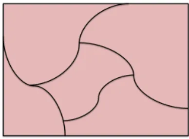
We note in passing that any finite space is trivially a quasi-discrete closure space. Quasi discrete closure spaces can be used to model spatial structures in Rn, as shown below. Example 2.28. LetF ⊆ ℘(Rn) be a partition of Rn, each element of which is either open or closed, i.e. ∪A∈FA = Rn, ∀A, B ∈F : A 6= B → A∩B = ∅, ∀A ∈ F : A = I(A)∨A = C(A).
We let RF ⊆F × F be the connectedness relation among elements of F , formally: RF = {(A, B)|A, B open and C(A) ∩ C(B) 6= ∅}
where C is the standard topological closure over Rn. It is easy to see that (F , CRF) is a quasi discrete closure space. Figure 3 shows an example in R2, where the open sets are shown in pink, while the only closed set is shown in black.
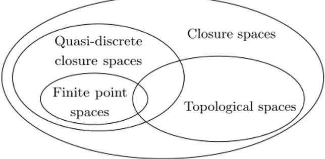
In Figure 4, the hierarchy of closure spaces with respect to quasi-discreteness is shown. All finite spaces are quasi-discrete, as closure of arbitrary sets is determined by that of the singletons, by the axiom C(A) ∪ C(B) = C(A ∪ B). Obviously there are quasi-discrete infinite spaces (any infinite graph interpreted as a closure space is an example). A quasi-discrete space which is also topological is the space associated to any complete graph. In this case, for any set, C(A) is the whole space, thus closure is idempotent. More precisely, the topology determined by the closure operator associated to a complete graph is the indiscrete topology, where the only open sets are the empty set and the whole space. It is obvious that there are topological spaces that are not quasi-discrete, such as Euclidean spaces. Finally there are closure spaces that are neither topological nor quasi discrete. The most obvious example is
Closure spaces Topological spaces Quasi-discrete closure spaces Finite point spaces
Figure 4: The hierarchy of closure spaces.
the coproduct (disjoint union) of a topological space which is not quasi-discrete (e.g. any Euclidean space), and a quasi-discrete, but not topological, closure space. The disjoint union of two closure spaces is defined below (we omit the proof that it actually obeys to the axioms of a closure space, as it is an easy exercise).
Definition 2.29. Given two closure spaces (X, CX) and (Y, CY), consider the disjoint
union of X and Y , represented as X ] Y = X0 ∪ Y0 with X0 = {(1, x) | x ∈ X} and Y0 = {(2, y) | y ∈ Y }. In order to equip the set X ] Y with a closure operator, for each A ⊆ X ] Y , let AX = {x | (1, x) ∈ A} and AY = {y | (2, y) ∈ A}. Define C(A) = {(1, x) | x ∈ CX(AX)} ∪ {(2, y) | y ∈ CY(AY)}.
2.4. Paths and connectedness in closure spaces. In this section we define paths and connectedness for interesting classes of closure spaces. A uniform definition of paths in closure spaces is non-trivial. It is possible, and often done, to borrow the notion of path from topology. However, as we shall see, the extension is not fully satisfactory. For example, the topological definition does not yield graph-theoretical paths in the case of quasi-discrete closure spaces. Our solution is pragmatic. We define paths as it is natural in interesting classes of closure spaces. We leave open the possibility to change this notion, in chosen classes of closure spaces, practically making our theory dependent on such choice. The theoretical question of finding a truly uniform notion of path (e.g., by some form of category-theoretical universal property characterising a path-connected class of spaces) is left for future work. First of all we introduce the definition of continuous function, which restricts to topological continuity in the setting of idempotent closure spaces3.
Definition 2.30. A continuous function f : (X1, C1) → (X2, C2) is a function f : X1 → X2
such that, for all A ⊆ X1, we have f (C1(A)) ⊆ C2(f (A)).
Below, two kinds of paths are introduced: Euclidean paths and quasi-discrete paths. Definition 2.31. For each closure space (X, C), assume a chosen closure space I, equipped with a linear order ≤ with bottom 0, and call path a continuous function p : I → (X, C). In particular, call Euclidean path any continuous function whose domain is the half-line R≥0 = {x ∈ R | 0 ≤ x}, equipped with the Euclidean (topological) closure operator. Call 3Note that in topological spaces one may equivalently use the definition we propose here, based on the
Kuratowski axioms, or the definition of continuity using open sets, namely f is continuous whenever for each open set o, f−1(o) is open. However, the two definitions do not coincide for arbitrary closure spaces (open sets play a less important role in closure spaces, see Remark 2.19).
quasi-discrete path any continuous function whose domain is the quasi-discrete closure space (N, CSucc) where (n, m) ∈ Succ ⇐⇒ m = n+1. Whenever (X, C) is an Euclidean topological
space (resp. a quasi-discrete closure space), call path an Euclidean (resp. quasi-discrete) path whose codomain is (X, C).
Note that in Definition 2.31 we do not require compatibility conditions between the closure operator and the linear order of I. Depending on the application context, different orders may be chosen, obtaining different interpretations of logics, or different degrees of compatibility between closure and paths (see e.g. Theorem 3.7). We consider the study of appropriate compatibility conditions, determining a universal notion of path for certain classes of closure spaces, out of scope for the current paper. We can, though, provide a hint about the complexity of such study. One of the major difficulties in finding a unifying notion is that Euclidean paths are not directed, whereas quasi-discrete paths are directed. The examples in this section are also aimed at making this problem more clear. Directed paths in topology are a highly non-trivial topic by themselves, and gave rise to the subject of directed algebraic topology [Gra09]. Generalizing directed algebraic topology to work in the setting of closure spaces could be a relevant strategy to face these issues.
As a matter of notation, we call p a path from x, and write p : x ∞, when p(0) = x. We write y ∈ p whenever there is i such that p(i) = y. We also write p : x i
y ∞ when p is a
path from x and p(i) = y.
The definition of Euclidean path is intuitively similar to the classical topological definition of a path, namely a continuous function from the unit interval [0, 1], except that Euclidean paths that we defined are “open-ended on the right” (note that the open interval [0, 1) and R+ are continuously isomorphic). The definition of quasi-discrete path, on the other hand, mimics the classical definition of infinite path in a graph. Simply adopting Euclidean paths in quasi-discrete spaces yields counter-intuitive results, as shown below.
Example 2.32. Consider the quasi-discrete closure space obtained from the graph G = ({a, b}, {(b, a)}) having two nodes a, b, and only one edge, from b to a. Note that there is no graph-theoretical path from a to b. However, consider the function p : R≥0→ {a, b}, defined
by p(0) = a, and p(i) = b for i 6= 0. This function is continuous, thus it is an Euclidean path starting from a and traversing b. To see this, choose any subset J of the half-line.
• If J = ∅, the thesis is trivially obtained; otherwise, assuming J 6= ∅:
• if J = {0}, then p(C(J )) = p({0}) = p(J ) ⊆ C(p(J )); otherwise, assuming J 6= ∅ and J 6= {0}, necessarily b ∈ p(J ), and:
• if 0 /∈ J and 0 /∈ C(J ), then p(C(J )) = p(J ) = {b} ⊆ C(p(J )); • if 0 /∈ J and 0 ∈ C(J ), then p(C(J )) = {a, b} = C({b}) = C(p(J )); • if 0 ∈ J , then p(C(J )) ⊆ {a, b} = C(p(J )).
We saw that Euclidean paths may not yield the expected results in quasi-discrete closure spaces. On the other hand, graph-theoretical and quasi-discrete paths coincide.
Lemma 2.33. Given a (quasi-discrete) path p in a quasi-discrete space (X, CR), for all
i ∈ N with p(i) 6= p(i + 1), we have (p(i), p(i + 1)) ∈ R, i.e., the image of p is a (graph theoretical, countably infinite) path in the graph of R. Conversely, each countable path in the graph of R uniquely determines a quasi-discrete path.
Note that, in particular, in Example 2.32 there is no quasi-discrete path rooted in a and passing by b, whereas there are quasi-discrete paths rooted in b and passing by a (for
example, the path defined by p(0) = b and p(i > 0) = a). Let us introduce the notion of connectedness that we use in this work.
Definition 2.34. Given a closure space (X, C), set A ⊆ X is path-connected if and only if for each x, y ∈ A there is a path p and an index i such that p(0) = x, p(i) = y and, for all j ≤ i, p(j) ∈ A.
Note that, for quasi-discrete closure spaces, by Lemma 2.33, Definition 2.34 coincides with the usual notion of strong connectedness in graph theory.
Remark 2.35. It is worth mentioning that connectedness can be also borrowed from topology, resorting to the notion of separation. Formally, let (X, C) be a closure space. Two sets A1, A2 ⊆ X are separated if and only if C(A1) ∩ A2 = ∅ = A1 ∩ C(A2). Note
that separated sets are also disjoint, since for all sets A, we have A ⊆ C(A). Thus, there is no explicit requirement that A1 and A2 are disjoint. Set A ⊆ X is connected if and
only if there are no non-empty, separated sets A1, A2 ⊆ X such that A = A1∪ A2. In the
case of topological spaces, the difference between this definition and path connectedness is widely known. There is a difference also in quasi-discrete closure spaces. A quasi-discrete closure space which is connected, but not path-connected is the space ({1, 2, 3}, CR), where
R = {(1, 2), (3, 2)}. By Lemma 2.33 there is no path from 1 to 3; however, it is not possible to find two non-empty, separated sets A1, A2 with X = A1∪ A2. The only possible
choices, recalling that separated sets must be disjoint, are A1 = {1, 2}, A2 = {3}, with
C(A2) ∩ A1 = {2}, A1= {1}, A2 = {2, 3}, with C(A1) ∩ A2 = {2}, and A1 = {1, 3}, A2 = {2}
with C(A1) ∩ A2= {2}.
3. Spatial logics for closure spaces
In this section we present SLCS: a Spatial Logic for Closure Spaces, that we first proposed in [CLLM14a]. The logic is meant to assign to formulas a local meaning; for each point, formulas may predicate both on the possibility of reaching other points satisfying specific properties, or of being reached from them, along paths of the space. In [CLLM14a], SLCS is equipped with two spatial operators: a “one step” modality, called “near” and denoted by N , turning the closure operator C into a logical operator, and a binary spatial until operator U , which is a spatial counterpart of the temporal until operator. In the present paper we extend SLCS with an additional binary operator, P, used to model propagation, and propose a new interpretation for U , based on the notion of paths that we introduced in Section 2.4. In order to avoid confusion, we call the newly defined connective surrounded, and use the symbol S. Operator S coincides with U in the case of quasi-discrete closure spaces, and enhances it by also providing an intuitively meaningful interpretation in the case of continuous (e.g. Euclidean) spaces. The proposed spatial logic combines these new operators with standard boolean operators. Assume a finite or countable set AP of atomic propositions.
Definition 3.1. The syntax of SLCS is defined by the grammar in Figure 5, where a ranges over AP .
In Figure 5, > denotes the truth value true, ¬ is negation, ∧ is conjunction, N is the closure operator, S is the surrounded operator, and P is the propagation operator. From now on, with a small overload of notation, we let Φ denote the set of SLCS formulas. We shall now define the interpretation of formulas.
Φ ::= a [Atomic proposition] | > [True] | ¬Φ [Not] | Φ ∧ Φ [And] | N Φ [Near] | Φ S Φ [Surrounded] | Φ P Φ [Propagation] Figure 5: SLCS syntax
Definition 3.2. A closure model is a pair M = ((X, C), V) consisting of a closure space (X, C) and a valuation V : AP → 2X, assigning to each atomic proposition the set of points where it holds.
Definition 3.3. Satisfaction M, x |= φ of formula φ ∈ Φ at point x ∈ X in model M = ((X, C), V) is defined by induction on the structure of terms, by the equations in Figure 6. M, x |= a ∈ AP ⇐⇒ x ∈ V(a) M, x |= > ⇐⇒ true M, x |= ¬φ ⇐⇒ M, x 6|= φ M, x |= φ1∧ φ2 ⇐⇒ M, x |= φ1 and M, x |= φ2 M, x |= N φ ⇐⇒ x ∈ C({y ∈ X|M, y |= φ}) M, x |= φ1S φ2 ⇐⇒ M, x |= φ1∧ ∀p : x ∞.∀l.M, p(l) |= ¬φ1 =⇒ ∃k.0 < k ≤ l.M, p(k) |= φ2 M, x |= φ1P φ2 ⇐⇒ M, x |= φ2∧ ∃y.∃p : y l x ∞.M, y |= φ1∧ ∀i.0 < i < l =⇒ M, p(i) |= φ2 Figure 6: SLCS semantics
Atomic propositions and boolean connectives have the expected meaning. For formulas of the form φ1S φ2, the basic idea is that point x satisfies φ1S φ2 whenever there is “no
way out” from φ1 unless passing by a point that satisfies φ2. For instance, if we consider
the model of Figure 2, yellow nodes should satisfy yellow S red while green nodes should satisfy green S blue. A point x satisfies φ1P φ2 if it satisfies φ2 and it is reachable from a
point satisfying φ1 via a path such that all of its points, except possibly the starting point,
satisfy φ2. For instance, if we consider again the model of Figure 2, blue, green and white
nodes satisfy green P ¬red while the same formula is not satisfied by yellow nodes.
In Figure 7, we present some derived operators. Besides standard logical connectives, the logic can express the interior (Iφ), the boundary (δφ), the interior boundary (δ−φ) and the closure boundary (δ+φ) of the set of points satisfying formula φ. Moreover, by appropriately using the surrounded operator, operators concerning reachability (φ1R φ2),
global satisfaction (E φ, everywhere φ) and possible satisfaction (F φ, somewhere φ) can be derived. Finally we define the A connective, expressing that φ2 keeps x “apart” from φ1.
⊥ , ¬> φ1∨ φ2 , ¬(¬φ1∧ ¬φ2)
Iφ , ¬(N ¬φ) δφ , (N φ) ∧ (¬Iφ)
δ−φ , φ ∧ (¬Iφ) δ+φ , (N φ) ∧ (¬φ)
φ1R φ2 , ¬((¬φ2) S(¬φ1)) E φ , φ S ⊥
F φ , ¬ E(¬φ) φ1A φ2 , ¬(φ1P(¬φ2))
Figure 7: Some SLCS derived operators
Proposition 3.4. We have that:
(1) M, x |= φ1R φ2 if and only if there is p : x ∞ and k such that M, p(k) |= φ2 and for
each j with 0 < j ≤ k, we have M, p(j) |= φ1;
(2) M, x |= φ1A φ2, if and only if M, x |= φ2 or for any y such that M, y |= φ1, and for
any p : y l
x ∞, there exists i such that 0 < i < l and M, p(i) |= φ2.
(3) M, x |= E φ1 if and only if for each p : x ∞ and i ∈ N, M, p(i) |= φ1;
(4) M, x |= F φ1 if and only if there is p : x ∞ and i ∈ N such that M, p(i) |= φ1.
Note that point x satisfies φ1R φ2 if and only if either φ2 is satisfied by x or there exists
a sequence of points after x, all satisfying φ1, leading to a point satisfying both φ2 and φ1.
In the second case, it is not required that x itself satisfies φ1. For instance, both red and
green nodes in Figure 2 satisfy (white ∨ blue) R blue, as well as the white and blue nodes. The formula is not satisfied by the yellow nodes. This is so because the first node of a path leading to a blue node is not required to satisfy white or blue. It is easy to strengthen the notion of reachability when we want to identify all white nodes from which a blue node can be reached by requiring in addition that the first node of the path has to be white. We can define this notion as a derived operator as follows:
φ1T φ2, φ1∧ ((φ1∨ φ2) R φ2)
Note also that φ2 is occurring also in the first argument of R. This is because satisfaction
of φ1R φ2 requires that the final node on the path satisfies both φ1 and φ2.
A point x satisfies M, x |= φ1A φ2 if it satisfies φ2 or every path from a point y satisfying
φ1 to x passes by a point satisfying φ2, located between y and x. For instance, with reference
to Figure 2, let us consider yellow A red , that is ¬(yellow P ¬red ). Note that yellow P ¬red is satisfied by the yellow points in the figure: for each yellow point x, let y be any yellow point (even x itself) and p a path starting from y and passing by x staying in the yellow area. Furthermore, points that are not yellow do not satisfy yellow P ¬red by definition of P. Therefore, yellow A red is satisfied by all other points in the figure, including the red ones. Furthermore, all white nodes in the figure satisfy both yellow A red and green A blue.
It is worth noting that in some situations, operators dealing with paths in opposite directions may be inter-expressible. However, an appropriate formalisation of such kinds of axioms, and the study of the associated classes of closure models, is left for future work.
We conclude this section by restricting our attention to quasi discrete closure models, i.e. closure models that are originated from quasi discrete closure spaces, in order to compare Definition 3.3 with the interpretation of S studied in [CLLM14a].
Definition 3.5. A quasi discrete closure model is a pair M = ((X, C), V) consisting of a quasi discrete closure space (X, C) and a valuation V : AP → 2X, assigning to each atomic proposition the set of points where it holds.
Example 3.6. For k, h ∈ N, let N2
k,h be the set {(i, j) ∈ N × N | i ∈ [1, k] ∧ j ∈ [1, h]}. A
digital image of size k × h, on finite set of colours C, is a function f : N2k,h→ C, assigning a
colour to each point of a finite rectangle in N2. Such an image gives rise to the quasi-discrete closure space (Nk,h, C4adj), where
((x1, y1), (x2, y2)) ∈ 4adj ⇐⇒ (x1− x2)2+ (y1− y2)2= 1
Furthermore, we also define the closure model ((Nk,h, C4adj), V) with atomic propositions in
C, where V(c ∈ C) = {(i, j) ∈ N2k,h| f (i, j) = c}.
In words, such closure model is based on a regular grid, where each pixel, except those on the borders, has four neighbours, corresponding to the directions right, left, up and down. On top of this space, atomic propositions are interpreted as the colours of pixels.
In [CLLM14a], we introduced the spatial until operator φ1U φ2, with a similar intended
meaning as S. The main difference is that the definition of U requires existence of a set of points satisfying φ1, having closure boundary satisfying φ2. The definitions of S and U
coincide in the case of quasi-discrete spaces (see Theorem 3.7). As we will see, the definition using paths behaves in a more natural way for topological spaces. First, we compare the interpretation of S given in [CLLM14a] with Definition 3.3.
Theorem 3.7. In a quasi-discrete closure model M: M, x |= φ1S φ2 according to
Defini-tion 3.3 if and only if M, x |= φ1U φ2 according to [CLLM14a], namely, there is A ⊆ X such
that x ∈ A, and ∀y ∈ A.M, y |= φ1, and ∀z ∈ B+(A).M, z |= φ2.
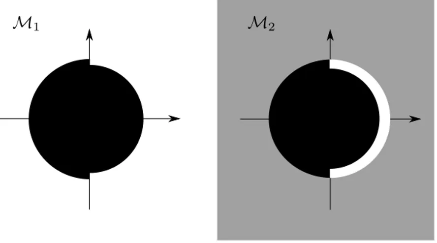
We conclude this section by showing two examples where the definition of [CLLM14a] behaves in a counter-intuitive way, whereas the definition using paths works as expected. Example 3.8. We define two models based on the Euclidean topology over R2, seen as a closure space (R2, C). We use propositions b, w, g, depicted in Figure 8 as black, white and grey areas, respectively. Consider the sets H = {(x, y)|x2+ y2 < 1}, H<= {(x, y)|x2+ y2 = 1 ∧ x < 0}, H≥ = {(x, y)|x2+ y2 = 1 ∧ x ≥ 0}. Let Mi = ((R2, C), Vi), for i ∈ {1, 2}.
Fix valuations as follows: V1(b) = H ∪ H<, V1(w) = R2\ V1(b), V1(g) = ∅, V2(b) = V1(b),
V2(w) = H≥, V2(g) = R2\ (H ∪ H<∪ H≥). Let x ∈ H. Clearly, we have M1, x |= b S w,
and M2, x 2 b S w, as there are paths starting at a black point in M2 and reaching a grey
point, which does not satisfy b, without passing by white points. The expectation is that b U w holds at x in M1, which is true by the choice A = H ∪ H<, but note that B+(A) = H≥.
For this reason, we also have M2, x |= b U w by the choice A = H ∪ H<, which is not what
one would expect when thinking of the area H being “surrounded” by white points.
4. The collective spatial logic CSLCS
So far, the properties expressed by our logic refer to points in space, when considered individually. However, when looking at space, it is also natural to formulate properties of sets of points, considered as a collective entity. As we shall see, our notion of collectivity is that of a set of points that are inter-reachable by paths in the whole space. Therefore, not only connected sets are of interest to our logic, but also sets of isolated points or
Figure 8: Two continuous closure models (boundaries are deliberately represented as very thick, but the reader should think of them as infinitely thin).
components, that are subsets of path-connected sets satisfying given properties. Other logics predicating on sets of points include the family of region calculi (see [KKWZ07] for a comprehensive overview), describing properties of regular sets, and using mereotopological boolean connectives (e.g., “part of”, “boundary”, and so on). Such logics characterise regions of space. We explicitly divert from this research line, because we aim at characterizing local properties of points, fitting in the tradition of modal logics, and relating individuals to the collectivity they live in. Our choice of collective operators is driven by this principle, and is modulated by the requirement of a computationally feasible model checking procedure.
Getting into detail, given a closure model M = ((X, C), V), one may introduce “collective” formulas ψ (whose syntax and semantics will be clarified in the sequel) equipped with a collective interpretation, assigning a boolean valuation to the problem M, A |= ψ for each set of points A ⊆ X. We define the collective spatial logic of closure spaces CSLCS, which is interpreted on closure models. The logic has a collective fragment and an individual fragment. The collective fragment is evaluated on subsets of the set of points of the space. The individual fragment, which is evaluated on single points, is the logic SLCS defined in Section 3.
Definition 4.1. Fix a set AP of atomic propositions. The syntax of formulas is defined by
the grammar in Figure 9, where a ranges over AP . •
We deliberately use the same syntax for boolean connectives both in the individual and the collective fragment, as usage of either fragment is always clear from the context. Boolean operators are standard. The novel operators we propose are the share connective and the group connective. Let φ be an individual formula, and ψ a collective formula. Informally, φ −< ψ (read: φ share ψ) is satisfied by set A when the subset of points of A satisfying the individual property φ also satisfies the collective property ψ. Formula Gφ holds on set A when its elements belong to a group, that is, a possibly larger, path-connected set of points, all satisfying the individual formula φ.
The satisfaction relation of the logic for each collective formula ψ is given in the form M, A |=C ψ, where M is a closure model (see Definition 3.2), and A ⊆ X is a set of points.
Collective formulas Individual formulas
Ψ ::= > [True] Φ ::= a [Atomic proposition]
| ¬Ψ [Not] | > [True] | Ψ ∧ Ψ [And] | ¬Φ [Not] | Φ −< Ψ [Share] | Φ ∧ Φ [And] | GΦ [Group] | N Φ [Near] | Φ P Φ [Propagation] | Φ S Φ [Surrounded] Figure 9: CSLCS syntax.
Definition 4.2. Given a model M = ((X, C), V)), and A ⊆ X, collective satisfaction |=C is
given by the inductive definition below, where |= is the individual satisfaction relation of Definition 3.3: M, A |=C > M, A |=C ¬ψ ⇐⇒ M, A 2C ψ M, A |=C ψ1∧ ψ2 ⇐⇒ M, A |=C ψ1 and M, A |=C ψ2 M, A |=C φ −< ψ ⇐⇒ M, {x ∈ A | M, x |= φ} |=C ψ M, A |=C Gφ ⇐⇒ ∃B ⊆ X.A ⊆ B ∧ B is path-connected ∧ ∀z ∈ B.M, z |= φ
The definition of G requires the existence of a set B which is possibly larger than A. The intuition is that the elements of A are part of a larger “collective”, consisting of elements satisfying φ. We consider variants of connectedness as the most basic forms of collective and spatial property. In particular, we use path-connectedness, in line with the path-based interpretation of SLCS. Connectedness is “collective” in the sense that it is not merely determined by a property of the singletons composing a set, and it is not even preserved in subsets of a connected set. On the other hand, even though one could imagine all sorts of collective predicates on a model, we focus on (path-)connectedness, as it is completely determined by the structure of a closure space. For this reason, we consider it a fundamental collective property, deserving special treatment in the field of spatial logics, akin to the notion of transition in models of modal logics. Due to the restrictions that we introduce (mainly the strict layering of the collective and individual fragments) the logic CSLCS can be automatically verified at a computational cost which is comparable to that of SLCS. Using CSLCS one is able to check that given individuals are in the same area of space, and they share specific properties. Informally (and depending on the chosen closure model), this idea can be interpreted, for example, as: the fact that certain individuals are able to connect and act as a group; that they may follow the same route to reach a goal; that they are located all together in a protected environment; etc. Below, we develop this concept by the means of some derived operators. In Section 7 we provide some examples.
Definition 4.3. The following derived operators may be defined, where ψ1 and ψ2 are
collective formulas, and φ is an SLCS formula:
⊥ , ¬> [False]
ψ1∨ ψ2 , ¬((¬ψ1) ∧ (¬ψ2)) [Or]
∀φ , ¬φ −< G⊥ [Forall, Individually]
∃φ , ¬(∀¬φ) [Exists]
∅ , ∀⊥ [Empty]
The definition of ∀ uses the fact that the only set A such that M, A |= G⊥ is the empty set, which is trivially path-connected. This is made formal by the following lemma.
Lemma 4.4. We have:
(1) M, A |=C ∀φ if and only if ∀x ∈ A.M, x |= φ;
(2) M, A |=C ∃φ if and only if ∃x ∈ A.M, x |= φ;
(3) M, A |=C ∅ if and only if A = ∅.
The ∀ and ∃ connectives also exist in the classical topological logic S4u (see [KKWZ07]);
additionally, CSLCS provides the possibility to classify subsets, instead of whole models. However, global satisfaction, defined on models, is obtained as a side effect.
Definition 4.5. Global satisfaction is defined for each model M = ((X, C), V) and collective formula ψ as M |=Gψ ⇐⇒ M, X |=C ψ.
From now on, we will sometimes omit the subscripts C and G from the satisfaction relation, when clear from the context. Apart from the usual derived connectives, such as disjunction or logical implication, CSLCS can express some useful derived operators. Definition 4.6. Define the following collective derived operators:
φ1CS φ2 , G(¬φ2∧ (φ1S φ2)) [Collectively surrounded]
φ1CP φ2 , ∀((φ1∨ φ2) ∧ ¬(φ1∧ φ2))∧ [Collectively partitioned]
(φ1 −< (φ1CS φ2)) ∧ (φ2 −< (φ2CS φ1))
A set A satisfies M, A |= φ1CS φ2 if and only if the points in A satisfy φ1, and are
“collectively” surrounded by a set of points satisfying φ2. More precisely, using the connective
G, it is required that a path-connected set B including A exists, with all points of B satisfying φ1S φ2, but not φ2. Not only there can be no path rooted in B and leaving φ1 without
passing by φ2, but also, noting that all the elements of B satisfy φ1∧ ¬φ2, such set B must
be a path-connected component of ¬φ2, the elements of which are surrounded in the sense
of SLCS by points satisfying φ2.
For the CP connective, we look at its global interpretation. The statement M |= φ1CP φ2
expresses that all the points of the space satisfy either φ1or φ2, that all the points satisfying
φ1 can be connected to each other, forming a set of points satisfying φ1 and surrounded by
points satisfying φ2, and vice-versa. The sets of points satisfying φ1 is path-connected, and
so is the set satisfying φ2. For example, the model in the left-hand side of Figure 10 satisfies
red CP blue while the model in the right-hand-side of the figure does not satisfy the same formula.
Figure 10: The model on the left satisfies red CP blue; the one on the right does not.
Figure 11: A graphical representation of Example 5.1.
5. Example: emergency evacuation
In this section we show some examples of interpreting SLCS and CSLCS on quasi-discrete closure spaces. First, starting from our running example, let us define a closure space to provide a simple model of short-range communication.
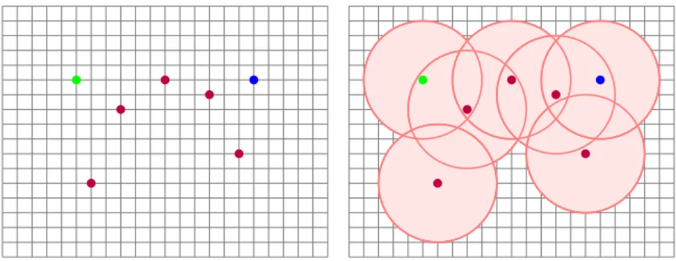
Example 5.1. Let us consider again the closure space presented in Example 2.6. This closure space can be used to model a network of agents distributed over a two-dimensional physical space, that communicate via wireless devices having fixed communication radius δ. In the left hand side of Figure 11 a graphical representation of such model is provided. There green, purple and blue dots identify different kinds of agents located in the space. Let us consider the colours as atomic propositions.
The set Cδ(green ∪ purple ∪ blue) consists of points in R2 that are in the communication
range of at least one agent, represented by the pink area in the right-hand side of Figure 11. Suppose that the green agent of our example is the source of some relevant information, which is meant to be transmitted from the green device to the other devices that are reachable after some hops. The set of devices that can receive the information sent by the green device is characterised, using the propagation operator, by the formula green P(purple ∪ blue), satisfied by the black points in Figure 12.
Taking advantage of both Example 3.6 (interpreting digital images as closure models) and Example 5.1, we will now set up a more complex closure space, comprising a communication layer, with closure determined by communication ranges, and a physical layer, with closure determined by the structure of a regular grid. The two layers are linked by a binary relation. On top of this set-up, we will discuss the interpretation of some example properties, assuming that a set of agents (modelled by appropriate atomic propositions) is distributed in the physical layer.
Example 5.2. Recall from Example 3.6 that digital images can be treated as finite quasi-discrete closure models. Consider one such model, with underlying space (X, C4adj), with
Figure 12: In black the devices that can receive data from the green device.
Figure 13: A representation of agents in a building in an emergency condition.
X ⊂ N2. In this example, we will use a digital image representing a portion of a two-dimensional physical space; therefore, each point of the image is also mapped to a position, or coordinate, in the Euclidean space R2, giving rise to a function map : X → R2. Let Y be the finite image of the function map. Assume X and Y are disjoint, for simplicity. Let pos be the graph of the function map, that is, the set of pairs {(x, y) ∈ X × Y | map(x) = y}. In a similar way as in Example 5.1, fix a communication range δ, and introduce the relation Rδ ⊆ R2 from Example 2.24. Then, let R0δ = Rδ∩ Y2 be the restriction of Rδ to the image
of the function map. Consider the set Z = X ∪ Y . Define the quasi-discrete closure space (Z, CR) using the relation
R , 4adj ∪ pos ∪ R0δ
The closure space (Z, CR) can be thought of as “two-layered”. One layer is the digital
image, the other one is a finite subset of R2 equipped with the closure Cδ restricted to Y ,
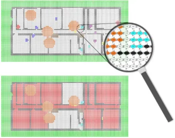
in a similar way to Example 2.6 . The two layers are linked by the relation pos; note that each position in Y is thus “close”, in the sense of the operator N , to a point of the digital image. By this, as we shall see, logic formulas can simultaneously predicate on proximity in the image, acting as a “physical” layer, where proximity means adjacency in space, and in Euclidean coordinates, acting as a “communication” layer, where proximity is based on distance. We will also consider a set of agents, first-aid facilities, obstructions, and dangerous areas, formalised as atomic propositions, giving rise to a quasi-discrete closure model.
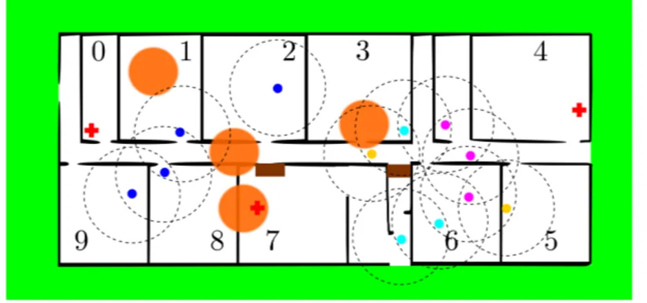
Before making this idea formal, we look at a picture of an instance of such construction, in Figure 13. The digital image in the background, the points of which form the set X, represents the map of a building at a specific instant in time, where an emergency situation occurs (note that rooms have been numbered for reader’s convenience, but we are not considering numbers, graphically, as part of the underlying map). The white points form the areas where agents can walk. Some of the white points, however, are covered by obstructions, painted in brown, or are in the range of some source of hazard. Hazardous areas are painted in semi-transparent orange. The green points are a safe area, accessible via exit doors. Some white points are also part of areas where first aid is available, which are represented by a red cross. The walls are painted in black. Coloured (blue, cyan, purple, yellow) dots represent agents, with their communication range (dashed circles). The set Y is the set of actual coordinates of the points in space denoted by pixels of the digital image.
We define a valuation function V, obtaining the quasi-discrete model ((Z, CR), V). Atomic
propositions are the colours white, black, green, red, blue, cyan, purple, yellow, brown, agent, danger, and coord. Function V is such that each point in the image satisfies its own colour. Proposition danger is true only at points in the image under the orange semi-transparent circles. Each point may satisfy more than one atomic proposition; in particular, points under the orange circles also satisfy other atomic propositions. Agents are represented by additionally colouring points of X in blue, cyan, purple, or yellow. Points that satisfy red or brown also satisfy white, as in principle these are areas where it is possible to walk, even though there is an obstruction in the current situation. Points of Y satisfy just one predicate, namely coord, and are not represented in Figure 13. In addition, no other point in Z satisfies predicate coord. Finally, define the short-hands obstacle , black ∨ brown ∨ danger, agent , blue ∨ cyan ∨ purple ∨ yellow, and safe , white ∧ ¬obstacle.
In this situation, we suppose that groups of agents of the same colour are expected to address an emergency situation together. Agents must be able to reach both first-aid points and exit doors without passing by dangerous areas. Agents belonging to the same group should reach a first-aid point and the exit together with other members of the group; in case an agent is isolated from her group, an agent of another group must be able to reach first aid, and then rescue her.
We remark that, for simplicity, when dealing with paths concerning agents, we do not consider the cases in which an agent may exit and re-enter the building through a different access, passing by the green area4. In the remainder of this section, we present some example properties, and their interpretation in the situation of Figure 13. First, recall the definition of the derived operator φ1T φ2 , φ1∧ ((φ1∨ φ2) R φ2). Point x satisfies φ1T φ2 whenever it
satisfies φ1 and there is a path p, and an index i, with p(0) = x, such that, for all j ∈ (0, i),
point p(j) satisfies φ1∨ φ2, and point p(i) satisfies φ2. Informally speaking, we may say that
T expresses reachability in space from a point satisfying formula φ1 to a point satisfying φ2,
only passing by points satisfying φ1 or φ2.
Example 5.3. There may be safe points, with no escape route. This is defined as the formula
φ1 , safe S obstacle
satisfied by the white points in Room 3.
4Depending on the application domain, one may take into account agents that exit and re-enter the
building by using another set of logical properties (the logic easily distinguishes between these two different kinds of paths).
Example 5.4. The walking areas, from which a first-aid point can be safely reached, are classified by the derived operator R. Consider the formula:
φ2 , safe T (red ∧ safe)
Points satisfying formula φ2 are required to be safe, and furthermore, to be at the start of a
path of safe points, leading to a point which is red and safe. In Figure 13, φ2 is satisfied,
among other points, by all the positions of agents, except those in rooms 3 and 7. That is, φ2 is satisfied by those white points that are the start of a path that avoids obstacles
(including dangerous areas), leading to safe first-aid facilities, while only traversing white points. Similarly, the points from which an exit may be reached are characterised by the formula
φ3, safe T green
which is satisfied by the blue, yellow, and violet points, but not by any cyan point (note that we are not considering the possibility of passing by the green area and re-enter the building, as we explained earlier). The points where first-aid facilities are located, and from where it is possible to safely reach an exit (all the red points in Figure 13), satisfy the formula
φ4 , (red ∧ safe) ∧ (safe T green)
Combining φ2 and φ4 one is then able to define the set of points from which one can safely
walk to a first aid point and then to the exit. These points are identified by the formula φ5 , safe T φ4
For instance, the white points in Room 8, but not those in Room 7, satisfy φ5.
We shall now introduce some collective formulas, that for simplicity are evaluated under the global interpretation of Definition 4.5.
Example 5.5. We can define a collective formula, parametrised by a colour, that is true whenever all agents of the given colour are connected in the communication layer of the model.
φ6(colour) = (coord ∧ N colour) −< G(coord ∧ N agent)
In the definition of φ6, note that N colour denotes the set of points that are near to a point
satisfying colour. Such set is the union of the points in the digital image where the agents of the given colour are located, their neighbours in the digital image, and their coordinates in the communication layer. Therefore, when colour is the colour of an agent, the sub-formula coord ∧ N colour precisely identifies the coordinates in Y that are positions of agents in the group identified by colour. Such coordinates are required to be part of a larger set of points, which are connected in the communication layer, and also are positions of arbitrary agents, so that the communication flow required by the formula may also include agents of different colours. In the model of Figure 13, φ6(colour) holds for all the colours of agents, except
blue.
Example 5.6. Agents of the same colour should be able to reach a first aid point, and then an exit, all together. We leave the colour as a parameter of the formula.
φ7(colour) = colour −< Gφ5
Example 5.7. We shall now deal with rescuing of agents. An agent of a given colour can be rescued if there is an agent of a different colour that can reach her, after passing by a first-aid point, and the two can safely reach an exit. First consider formula φ8(colour),
describing first-aid points that can be reached by an agent of a different colour than the given one (this is achieved by the sub-formula agent ∧ (¬colour) below), by a safe route:
φ8(colour) , (red ∧ ¬obstacle) ∧ (N ((agent ∧ (¬colour)) P safe))
Points satisfying φ8(colour) are red and not an obstacle, that is, they are safe first-aid
locations. Furthermore, the definition of φ8(colour) also uses the P operator in order to
guarantee that such points are directly connected (operator N ) to points that can be reached5 from a point where an agent of a different colour is located, passing only through safe points. Thus, agents of a specific colour that can be rescued satisfy the formula
φ9(colour) , agent ∧ φ2∧ N (¬obstacle ∧ (φ8(colour) P safe))
We can also define a collective formula expressing that, for a given colour, either φ7(colour)
holds, or all agents can be rescued:
φ10(colour) , φ7(colour) ∨ ∀(colour −< φ9(colour))
In our example model, φ10(blue) is true, whereas φ10(cyan) is false.
6. Spatial model checking
In this section we describe a model checking algorithm for SLCS and CSLCS. The algorithm is composed of two procedures, one for individual formulas, that is, the logic SLCS, and one for collective formulas, making use of the procedure for individual formulas. As we shall see, the procedure for individual formulas is a global model checking procedure for SLCS. Given model M = ((X, CR), V) and formula φ, the procedure returns the set {x ∈ X | M, x |= φ}. The
procedure for collective formulas, on the other hand, is a local model checking algorithm, that is, given model M, formula ψ and set of points A, it returns the boolean satisfaction value of M, A |= ψ. We choose a local algorithm for the collective fragment, since enumeration of a set of subsets is a problem of inherent exponential complexity. Merely returning a result for a global model checking procedure would require some kind of symbolic description, which is left for future investigation.
Function Sat, computed by Algorithm 1, implements the model checker for SLCS. The function takes as input a finite, quasi-discrete model M = ((X, CR), V) and a SLCS formula
φ, and returns the set of all points in X satisfying φ. The function is inductively defined on the structure of φ and, following a bottom-up approach, computes the resulting set via an appropriate combination of the recursive invocations of Sat on the subformulas of φ. When φ is of the form >, p, ¬φ1 or φ1∧ φ2, the definition of Sat(M, φ) is straightforward. To
compute the set of points satisfying N φ1, the closure operator C of the space is applied to
the set of points satisfying φ1. When φ is of the form φ1S φ2, function Sat relies on the
function CheckSurr defined in Algorithm 2. When φ is of the form φ1P φ2, function Sat
relies on the function CheckProp defined in Algorithm 3.
5Since the model of our example is symmetric, reachability in opposite directions may not make an actual
difference. However, models similar to the one we are depicting may feature e.g., one way doors. We are not adding one-way links in our model, as we do not deem it necessary for illustrating the connectives of the logic, and it makes the formal definition of the underlying closure space less readable.
Function Sat(M, φ)
Input: Finite, quasi-discrete closure model M = ((X, CR), V),
formula φ Output: Set of points
{x ∈ X | M, x |= φ} Match φ case > : return X case p : return V(p) case ¬φ1: let P = Sat(M, φ1) return X \ P case φ1∧ φ2: let P = Sat(M, φ1) let Q = Sat(M, φ2) return P ∩ Q case φ1P φ2: return CheckProp (M,φ1,φ2) case φ1S φ2: return CheckSurr (M,φ1,φ2) Function CheckSurr (M,φ1,φ2)
Input: Finite, quasi-discrete closure model M = ((X, CR), V),
formulas φ1, φ2
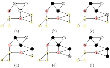
Output: Set of points {x ∈ X | M, x |= φ1S φ2} var V := Sat(M, φ1) let Q = Sat(M, φ2) var T := B+(V ∪ Q) while T 6= ∅ do var T0 := ∅ for x ∈ T do let N = pre(x) ∩ V V := V \ N T0 := T0∪ (N \ Q) T := T0; return V
Algorithm 1: Decision procedure for the model checking problem of SLCS.
Algorithm 2: Checking surrounded formulas in a quasi-discrete closure space.
Function CheckProp (M,φ1,φ2)
Input: Finite, quasi-discrete closure model M = ((X, CR), V), formulas φ1, φ2
Output: Set of points {x ∈ X | M, x |= φ1P φ2}
var V := Sat(M, φ1) var Q = Sat(M, φ2) var T := CR(V ) ∩ Q var R := T var Q := Q \ T while T 6= ∅ do var T0 := ∅ for x ∈ T do T0 := T0∪ (Q ∩ post(x)) Q := Q \ T0 R := R ∪ T0 T := T0 return R