Simulation Based Formal Verification of
Cyber-Physical Systems
PhD School in Computer Science, XXX Cycle
Faculty of Information Engineering, Informatics, and Statistics Department of Computer Science
Candidate Massimo Nazaria ID number 1086281
Thesis Committee
Prof. Enrico Tronci (Advisor) Prof. Toni Mancini
Prof. Gaia Maselli
External Reviewers Prof. Aniello Murano Prof. Patrizio Pelliccione
A thesis submitted in partial fulfillment of the requirements for the degree of Doctor of Philosophy in Computer Science
Copyright c 2018 Massimo Nazaria
Author’s Address Massimo Nazaria
Abstract
Cyber-Physical Systems (CPSs) have become an intrinsic part of the 21st century world. Systems like Smart Grids, Transportation, and Healthcare help us run our lives and busi-nesses smoothly, successfully and safely. Since malfunctions in these CPSs can have serious, expensive, sometimes fatal consequences, System-Level Formal Verification (SLFV) tools are vital to minimise the likelihood of errors occurring during the development process and beyond. Their applicability is supported by the increasingly widespread use of Model Based Design (MBD) tools. MBD enables the simulation of CPS models in order to check for their correct behaviour from the very initial design phase. The disadvantage is that SLFV for complex CPSs is an extremely time-consuming process, which typically requires several months of simulation. Current SLFV tools are aimed at accelerating the verifica-tion process with multiple simulators working simultaneously. To this end, they compute all the scenarios in advance in such a way as to split and simulate them in parallel. Fur-thermore, they compute optimised simulation campaigns in order to simulate common prefixes of these scenarios only once, thus avoiding redundant simulation. Nevertheless, there are still limitations that prevent a more widespread adoption of SLFV tools. Firstly, current tools cannot optimise simulation campaigns from existing datasets with collected scenarios. Secondly, there are currently no methods to predict the time required to com-plete the SLFV process. This lack of ability to predict the length of the process makes scheduling verification activities highly problematic. In this thesis, we present how we are able to overcome these limitations with the use of a simulation campaign optimiser and an execution time estimator. The optimiser tool is aimed at speeding up the SLFV process by using a data-intensive algorithm to obtain optimised simulation campaigns from existing datasets, that may contain a large quantity of collected scenarios. The estimator tool is able to accurately predict the execution time to simulate a given simulation campaign by using an effective machine-independent method.
Acknowledgements
First of all, I would like to thank my advisor Professor Enrico Tronci for his precious guidance and support over the past few years, and for being an immense source of inspira-tion with his excepinspira-tional technical-scientific knowledge and extraordinary human qualities. Secondly, my thanks go to my colleagues at the Model Checking Laboratory1 for their
prompt help whenever I needed it, and for providing me with a friendly-yet-professional work environment. Last but not least, I would like to thank my family and friends for their unconditional support, encouragement, and love without which I would never have come this far.
1
Table of Contents
Abstract ii
Acknowledgements iv
List of Figures viii
List of Tables ix
List of Acronyms x
1 Introduction 1
1.1 Framework . . . 1 1.2 Model Based System-Level Formal Verification . . . 2 1.3 State of the Art . . . 6 1.3.1 SLFV via Parallel Model Checking Driven Simulation . 6 1.3.2 Probabilistic Temporal Logic Falsification of CPSs . . . 11 1.4 Motivations . . . 12 1.5 Thesis Focus and Contributions . . . 12 1.5.1 Simulation Campaign Optimiser . . . 13 1.5.2 Simulation Campaign Execution Time Estimator . . . 13 1.5.3 Publications . . . 14 1.6 Outline . . . 15
2 Background 16
2.1 Notation . . . 16 2.2 Definitions . . . 16
3.1.3 Contributions . . . 21
3.2 Problem Formulation . . . 21
3.3 Methodology . . . 22
3.3.1 Overall Method . . . 22
3.3.2 Steps of the Algorithm . . . 23
3.3.3 Correctness of the Algorithm . . . 28
3.4 Experimental Results . . . 29
3.4.1 Computational Infrastructure . . . 30
3.4.2 Benchmark . . . 30
3.4.3 Optimisation Experiments . . . 30
3.4.4 Execution Time Analysis . . . 31
3.4.5 Optimisation Effectiveness Analysis . . . 33
3.5 Related Work . . . 34
3.6 Conclusions . . . 35
4 Execution Time Estimation of Simulation Campaigns 36 4.1 Introduction . . . 36 4.1.1 Framework . . . 36 4.1.2 Motivations . . . 37 4.1.3 Contributions . . . 38 4.2 Background . . . 39 4.2.1 Definitions . . . 39 4.2.2 Prediction Function . . . 40 4.3 Problem Formulation . . . 41 4.4 Methodology . . . 41 4.4.1 Overall Method . . . 42 4.4.2 Training Phase . . . 43 4.4.3 Prediction Function . . . 49 4.5 Experimental Results . . . 57
4.5.1 Validation of the Method . . . 57
4.6 Related Work . . . 61
4.7 Conclusions and Future Work . . . 62
4.7.1 Conclusions . . . 62
5 Conclusions and Future Work 63 5.1 Conclusions . . . 63
5.2 Future Work . . . 64
Appendices 65
A.1 Definitions . . . 66
A.2 Input Format . . . 67
A.3 Output Format . . . 68
A.4 Algorithm Steps . . . 70
A.5 Command-Line Tools . . . 75
A.5.1 dt-sort . . . 75 A.5.2 dt-label . . . 75 A.5.3 dt-optimise . . . 75 A.5.4 dt-merge . . . 76 A.5.5 Usage . . . 76 Bibliography 78
List of Figures
1.1 Simulation Based Verification . . . 3
1.2 Simulation Based System-Level Verification Process . . . 5
1.3 SLFV via Parallel Model Checking Driven Simulation . . . 7
3.1 Overall Execution Time for Optimisation . . . 31
3.2 Execution Time for each Optimisation Step . . . 32
3.3 Compression Ratio per Input Dataset . . . 33
4.1 Integration Steps to Simulate Command run(t) . . . 44
4.2 Execution Time to Simulate Commandrun(t) . . . 45
4.3 Execution Time Distribution of Command load . . . 52
4.4 Execution Time Distribution of Command store . . . 53
4.5 Execution Time Distribution of Command inject . . . 54
4.6 Execution Time Distribution of Command free . . . 55
4.7 Execution Time for Commands load, store, inject, and free . . 56
4.8 Average Prediction Error of runS . . . 58
List of Tables
2.1 Simulator Commands . . . 18
3.1 Overall Execution Time and CPU usage for Optimisation . . . 32
3.2 Compression Ratio per Input Dataset . . . 34
4.1 Values of t to Sample for Command run(t) . . . 48
4.2 Parameters of Prediction Function runS . . . 50
4.3 Average Prediction Error of runS . . . 58
4.4 Estimation Error of Simulation Campaings . . . 60
List of Acronyms
CPS Cyber-Physical System CCP Coupon Collector’s Problem DFS Depth-First Search
DT Disturbance Trace LBT Labels Branching Tree LCP Longest Common Prefix MBD Model Based Design
MCDS Model Checking Driven Simulation ODE Ordinary Differential Equations OP Omission Probability
PWLF Piecewise Linear Function RMSE Root-Mean-Square Error SBV Simulation Based Verification SLFV System-Level Formal Verification WCET Worst Case Execution Time
Chapter 1
Introduction
1.1
Framework
Over the past few decades, we have experienced many technological break-throughs which have revolutionised the way we live. Cyber-Physical Systems (CPSs) such as smart grid, automotive, and medical systems contribute to ensuring our lives run smoothly, safely and securely. They have become such an intrinsic part of our 21st century world, that few people nowadays could imagine living without them.
Consequently, we have come to expect CPSs to autonomously cope with all the faulty events originating from the environment they operate in. For example, control software in a car must be able to detect any hardware failure and take immediate mitigating action with a high level of autonomy.
In order to achieve this, software components must ensure that all the rele-vant faulty events from the external environment are promptly detected, and appropriately dealt with in such a way as to either prevent system failures, or recover from temporary malfunctions in a reasonable amount of time. Since malfunctions in these CPSs can have far-reaching, potentially danger-ous, sometimes fatal consequences, it is extremely important to use the most appropriate verification methods over the development life cycle. For this reason, verification activities are performed in parallel with the development process, from the initial design up to the acceptance testing stages.
This is particularly the case at the earliest design stages, where both the cost and effort required to fix design defects can be minimised. Furthermore, the propagation of undiscovered design defects over subsequent stages results in an exponential increase in the reworking needed to resolve them [18].
In fact, the verification of automobile components must prove that the car works as expected in any operating conditions, including engine speed, road surface and ambient temperatures. To this end, thousands of kilometers of road tests are typically needed to verify newly developed components on real vehicles.
Any bug found at this later verification stage has a huge impact on the project schedule and costs. In order to mitigate this, proper simulation methods are used to carry out verification activities as early as possible.
1.2
Model Based System-Level Formal
Verification
Verification methods and tools have long been established as the greatest contributing factor for any successful software development life cycle. Nowa-days, there are a variety of verification tools available for all the specific development stages, including system-level design, unit-level coding, integra-tion, and acceptance testing.
Model Based System-Level Formal Verification (SLFV) tools are extremely valuable to fulfil the need to verify the correctness of CPSs being developed during the earliest stages of the development process. One advantage of this model-based approach is that it brings verification forward in the develop-ment life cycle. Thus, developers are able to construct, test, and analyse their designs before any system component is implemented. In this way, if major problems are found, they can be resolved with less impact on the budget or schedule of the project.
The goal of SLFV is to use simulation to build confidence that the system as a whole behaves as expected regardless of disturbances originating from the operational environment. Examples of disturbances include sensor x has a failure, and parameter y has been changed. The fact that there are typically a huge number of disturbance scenarios that can originate from the environment makes SLFV of complex CPSs very time-consuming.
Simulation Based Verification
The most commonly used approach to carrying out SLFV is called Simulation Based Verification (SBV), which consists of simulating both hardware and software components of the CPS at the same time in order to reproduce all the relevant operational scenarios. As an example, Figure 1.1 shows a typical SBV setting. Controller (Software System) Plant (Physical System)
Simulator
Scenarios
Fail
Pass
Figure 1.1: Simulation Based Verification
The applicability of SLFV is supported by the increasing use of Model Based Design (MBD) tools to develop CPSs. This is particularly the case within the Automotive, Space, and High-Tech sectors, where tools like Simulink have been established as de facto standards. Such a widespread adoption of MBD tools is mainly due to the fact that they enable SLFV activities at an early stage in the development life cycle.
In this way, when designing a new feature for an existing CPS, modelling and simulation activities can be carried out in order to detect potential de-sign defects that would negatively impact the total development effort and cost. In fact, the re-working that would be required to resolve such defects increases exponentially, if the defects are able to propagate undiscovered over subsequent development stages.
stage implies significantly less cost and effort compared to later integration and acceptance testing stages.
Another advantage is clearly the potential for shorter time-to-market, which is useful for producers to accelerate getting their product to market so as to maximise the volume of sales after development kickoff.
Simulation Based Verification Process
Figure 1.2 illustrates a high-level diagram of a typical SBV process. In a nutshell, it consists of the following two main phases. First, theGeneration Phase where simulation scenarios are generated. Second, the Verification Phase where SBV is carried out.
In the case of failure, design errors are fixed and simulation is repeated until the final output is Pass.
Operational Environment and Safety Properties Specification SLFV uses formal languages to specify both the environment where the sys-tem will operate, and the safety properties it is necessary to satisfy, regardless of any faulty events originating in the specified environment. These formal specification languages include Simulink, and SysML1.
As a result of these specifications, SLFV can be performed using an assume-guarantee approach. Namely, an SLFV output of Pass guarantees that the system will behave as expected, assuming that all and only the relevant scenarios are formally specified.
1
Verification Phase Generation of Simulation Scenarios Simulation Fix Pass/Fail End Fail Pass 5
1.3
State of the Art
Notwithstanding the significant advantages of using SLFV, the verification of complex CPSs still remains an extremely time-consuming process. As a matter of fact, SLFV can take up to several months of simulation since it requires a considerable amount of scenarios to be analysed [4].
In order to mitigate this, techniques aimed at speeding up the SLFV process have recently been studied. The two approaches described below use formal methods to specify both the operational environment of the CPS and the safety properties to verify.
1.3.1
System-Level Formal Verification via Parallel
Model Checking Driven Simulation
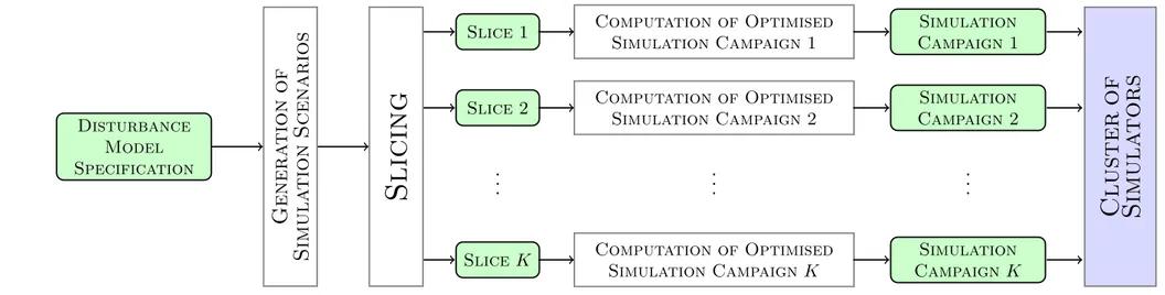
The approach shown in Figure 1.3 is the so-called Parallel Model Checking Driven Simulation (MCDS) method, which performs SLFV by using a black box approach. This is particularly useful to meet the need to exhaustively analyse the CPS behaviour in all the relevant scenarios that may arise within its operational environment.
This takes place during an initial offline phase where all such scenarios are generated. This upfront generation enables the resulting scenarios to be split into multiple chunks and then simulated in parallel [2][4]. Hence, the MCDS method accelerates the entire SLFV process by involving multiple computing resources which work simultaneously.
Furthermore, the generated scenarios are used to create optimised simulation campaigns with the aim of avoiding redundant simulation. Basically, these campaigns remove this redundancy by simulating duplicate scenarios only once. As a result, SBV is carried out more efficiently by reducing costs and time for simulation activities.
Disturbance Model Specification
Genera
tion
of
Simula
tion
Scenarios
Slicing
Cluster
o
f
Simula
tors
Slice 1 Slice 2 Slice K..
.
Computation of Optimised Simulation Campaign 1 Computation of Optimised Simulation Campaign 2 Computation of Optimised Simulation Campaign K..
.
Simulation Campaign 1 Simulation Campaign 2 Simulation Campaign K..
.
Figure 1.3: SLFV via Parallel Model Checking Driven Simulation
This optimisation is achieved by exploiting the ability of cutting-edge sim-ulation technology (e.g., Simulink2) to store the intermediate states of the simulation3. These intermediate states are then re-used as the starting point to simulate future scenarios, without the need to start from scratch [2]. Experimental results in [4] show that by using 64 machines with an 8-core processor each, this parallel MCDS approach can complete the SLFV activity in about 27 hours whereas a sequential approach would require more than 200 days.
On top of that, the following benefits can also be exploited from the MCDS method. For example, it can provide online information about the verification coverage, and the Omission Probability (OP) [3][5]. Namely, it can indicate both the number of scenarios simulated so far, and the probability of finding a yet-to-simulate scenario that falsifies a given safety property.
The approach to SLFV that is closest to the MCDS method is presented in [27], where the capability to call external C functions of the model checker CMurphi [12] is exploited in a black box fashion to drive the ESA satellite simulator SIMSAT4 in order to verify satellite operational procedures. Also in [34], the analogous capability of the model checker SPIN5 is used to verify actual C code. Both these approaches differ from the MCDS method since they do not consider the optimisation of simulation campaigns.
2https://www.mathworks.com/products/simulink.html
3Explanation of the store capability. If the developer clicks Start in the
Simulink toolbar, then the simulation begins. After a few seconds, if the developer clicks Pause in the same toolbar, then the simulation stops. At the same time, the simulator transparently stores the reached state of the simulation in the Simulink workspace. If the developer clicks Start again, then the simulator transparently loads the stored sim-ulation state, and then starts the simsim-ulation from the exact simsim-ulation state that was reached when the developer clicked Pause. Fortunately, these actions can be performed programmatically or via command-line, without the need to open the Simulink GUI.
4
http://www.esa-tec.eu/space-technologies/from-space/real-time-simulation-infrastructure-simsat/
5
Statistical and Monte Carlo model checking approaches
Statistical model checking approaches, being basically black box, are also closely related to the MCDS method. For example, [47] addresses SLFV of Simulink models and presents experimental results on the very same Simulink case studies that are used in this thesis. Monte Carlo model checking ap-proaches (see, e.g., [40][43][31]) are also related to this method as well. The main differences between these two latter approaches and the MCDS method are the following: (i) statistical approaches sample the space of admissible simulation scenarios, whereas MCDS addresses exhaustive SBV; (ii) statis-tical approaches do not address optimisation of the simulation campaign, despite the fact that it makes exhaustive SBV more viable.
Formal verification of Simulink models has been widely investigated, exam-ples are in [42][37][45]. These methods, however, focus on discrete time models (e.g., Simulink/Stateflow restricted to discrete time operators) with small domain variables. Therefore they are well suited to analyse critical subsystems, but cannot handle complex SLVF tasks (i.e., the case studies addressed in this thesis).
This is indeed the motivation for the development of statistical model check-ing methods as the one in [47] and for exhaustive SBV methods like the MCDS one. For example, in a Model Based Testing setting it has been widely considered the automatic generation of test cases from models (see, e.g., [26]). In SBV settings, instead, automatic generation of simulation scenarios for Simulink has been investigated in [30][35][25][44]. The main differences between these latter approaches and the MCDS method are the following. First, these approaches cannot be used in a black box setting since they generate simulation scenarios from Simulink/Stateflow models, whereas the MCDS method generates scenarios from a formal specification model of disturbances. Second, the above approaches are not exhaustive, whereas the MCDS method is.
Synergies between simulation and formal methods have been widely investi-gated in digital hardware verification. Examples are in [46][32][39][28] and citations thereof. The main differences between these latter examples and the MCDS method are: (i) they focus on finite state systems, whereas the MCDS method focuses on infinite state systems (namely, hybrid systems); (ii) they are white box (i.e., they require the availability of the CPS model
The idea of speeding up the SBV process by saving and restoring suitably selected visited states is also present in [28]. Parallel algorithms for explicit state exploration have been widely investigated. Examples are in [41][23][38][24][33]. The main difference between the MCDS method is that these latter ones fo-cus on parallelising the state space exploration engine by devising techniques to minimise locking of the visited state hash table whereas the MCDS method leaves the state space exploration engine (i.e., the simulator) unchanged, and uses an embarrassingly parallel (i.e., map and reduce like [29]) strategy that splits (map step) the set of simulation scenarios into equal size subsets to be simulated on different processors, and stops the SBV process as soon as one of these processors finds an error (reduce step).
The work in [48] also presents an algorithm to estimate the coverage achieved using a SAT based bounded model checking approach. However, since scenar-ios are not selected uniformly at random, it does not provide any information about the OP, whereas the MCDS method does.
Random model checking, Coverage, and Omission Probability Random model checking is a formal verification approach closely related to the MCDS method. A random model checker provides, at any time during the verification process, an upperbound to the OP. Upon detection of an error, a random model checker stops and returns a counterexample. Random model checking algorithms have been investigated, e.g., in [31][43][49]. The main differences with respect to the MCDS method are the following: (i) all random model checkers generate simulation scenarios using a sort of Monte-Carlo based random walk. As a result, unlike the MCDS method, none of them is exhaustive (within a finite time horizon); (ii) random model checkers (e.g., see [31]) assume the availability of a lower bound to the probability of selecting an error trace with a random-walk. Being exhaustive, the MCDS method does not make such an assumption.
The coverage yielded by random sampling a set of test cases has been studied by mapping it to the Coupon Collector’s Problem (CCP) (see, e.g., [50]). In the CCP, elements are randomly extracted uniformly and with replacement from a finite set of n test cases (i.e., simulation scenarios in the context of this thesis). Known results (see, e.g., [51]) tell us that the probability distribution of the number of test cases to be extracted in order to collect all n elements has expected value of Θ(n log n), and a small variance with known bounds. This allows the MCDS method to bound the OP during the SBV process.
Different from CCP based approaches, not only does the MCDS approach bound the OP, but it also grants the completion of the SBV task within just n trials. This is made possible by the fact that simulation scenarios are completely generated upfront.
1.3.2
Probabilistic Temporal Logic Falsification of
Cyber-Physical Systems
Another useful approach to speed up the verification process is the so-called falsification method [15]. Different from the approaches related to, and in-cluding, the MCDS method illustrated above, it uses techniques that are aimed at quickly identifying scenarios that falsify the given properties. In other words, these techniques search for operational scenarios where a given requirement specification is not met, hence the evaluation of the correspond-ing logical property is false. In this way, only a limited number of scenarios are considered, thus less simulation is carried out.
In conclusion, both the aforementioned MCDS and the falsification meth-ods use monitors to discover potential simulation scenarios where the CPS being verified violates a given specification (see, e.g., [36]). These monitors are typically developed manually in the language of the simulator such as the Simulink and Matlab languages. This is an error prone activity that can invalidate the entire verification process, because bugs in these moni-tors that are due to hand coding mistakes can lead to two significant errors. Firstly, they can result in false positives, i.e., simulation results of Pass which wrongly indicate that the system was able to work as expected under all the given operational scenarios. Secondly, they can result in false nega-tives, i.e., simulation results of Fail which wrongly points to a scenario were a given requirement was violated.
For this reason, ways to generate monitors directly from formal specifications have recently been presented [16][17][20][21][22]. Clearly, these automatically generated monitors are free of those bugs that are frequently introduced by hand coding.
1.4
Motivations
Despite the fact that SBV tools currently represent the main workhorse for SLFV, they are unlikely to become more widely adopted, unless two limiting factors are overcome.
First of all, the SLFV tool presented in [2] cannot optimise existing datasets, since they may contain a huge number of collected scenarios. In fact, no methods to obtain optimised simulation campaigns from such datasets have yet been studied in spite of the clear need to reduce the time for simula-tion activities while increasing the quality of these campaigns by removing redundant scenarios.
The second limitation that prevents wider use of current SLFV methods is the lack of prior knowledge of the time needed to complete simulations. The uncertainty surrounding the duration, makes scheduling SLFV activities problematic. For example, underestimating the time needed for simulation activities could result in missed deadlines and costly project delays. More-over, an overestimated time could result in meeting deadlines long before-hand, which means some resources allocated to the verification task would remain unused.
1.5
Thesis Focus and Contributions to
System-Level Formal Verification
In this thesis, our main focus is on control systems modelled in Simulink6, which is a widely used tool in the area of control engineering.
In order to overcome the aforementioned limitations in optimising existing datasets and estimating the time needed for SLFV tasks, we devised and implemented the two following tools: (i) a simulation campaign optimiser, and (ii) an execution time estimator for simulation campaigns.
6
1.5.1
Simulation Campaign Optimiser
The optimiser tool is aimed at speeding up the SLFV process by avoiding redundant simulation. To this end, we devised and implemented a data-intensive algorithm to obtain optimised simulation campaigns from existing datasets, that may contain a large quantity of collected scenarios. These resulting campaigns are made up of sequences of simulator commands that simulate common prefixes in the given dataset of scenarios only once. These commands include save a simulation state, restore a previously saved simu-lation state, inject a disturbance on the model, and advance the simusimu-lation of a given time length.
Results show that an optimised simulation campaign is at least 3 times faster with respect to the non-optimised one [2]. Furthermore, the presented tool can optimise 4 TB of scenarios in 12 hours using just one core with 50 GB of RAM.
1.5.2
Execution Time Estimator for Simulation
Campaigns
The estimator tool is able to perform an accurate execution time estimate using a partially machine-independent method. In particular, it analyses the numerical integration steps decided by the solver during the simulation. From this preliminary analysis, it first chooses a small set of simulator commands to simulate, and then it collects execution time samples in order to train a prediction function.
Results show that this tool can predict the execution time to simulate a given simulation campaign with an error below 10%.
1.5.3
Publications
The following papers on our two main contributions presented in this thesis are currently being finalised for submission in collaboration with Vadim Alimguzhin, Toni Mancini, Federico Mari, Igor Melatti, and Enrico Tronci.
1. A Data-Intensive Optimiser Tool for Huge Datasets of Simula-tion Scenarios. To be submitted to Automated Software Engineering. 2. Estimating the Execution Time for Simulation Campaigns with Applications to Simulink. To be submitted to Transactions on Modeling and Computer Simulation.
1.6
Outline
Chapter 2 illustrates background notions and definitions that are used within the thesis.
Chapter 3 presents our optimiser tool. In particular, it first shows the overall method we devised, then it gives details of the algorithm we implemented, finally it presents experimental results regarding the ef-ficiency, scalability, and effectiveness of the method.
Chapter 4 introduces our estimator tool. It gives a detailed description of the method we devised, then it explains how we validated it, finally it presents the experimental results of estimation accuracy.
Chapter 2
Background
2.1
Notation
In this thesis, we use [n] to represent the initial segment {1, 2, . . . , n} of natu-ral numbers. Often, we use N+ and R+ to denote the set of natural numbers and positive real numbers respectively. Sometimes, the list concatenation operator is denoted by ∪ when we deal with sequences instead of sets.
2.2
Definitions
Disturbance
Definition 2.2.1 (Disturbance). A disturbance is a number d ∈ N+∪ {0}.
A disturbance identifies an exogenous event (e.g. a fault) that we inject into the model being simulated. As an exception, when a disturbance d is zero, we inject nothing on the model, thus a zero indicates what we call the non-disturbance event.
Simulation Interval
Definition 2.2.2 (Simulation Interval). A simulation interval τ indicates a fixed amount of simulation seconds. Note that the amount of simulation sec-onds is usually different from the elapsed time the simulator takes to actually
simulate them. In fact, the elapsed time needed to simulate a given simula-tion interval τ may be higher or lower than τ , depending on the complexity of the simulation model.
Simulation Scenario
Definition 2.2.3 (Simulation Scenario). A simulation scenario (or simply scenario) is a finite sequence of disturbancesδ = (d1, d2, . . . , dH) with length
|δ| = H. These disturbances in δ are associated to H consecutive simulation intervals that have fixed-length τ . In particular, we inject the model with each disturbance di ∈ δ at the beginning of the i-th simulation interval.
Hence, we simulateτ ·H simulation seconds starting from the initial simulator state, while injecting the model with disturbances at the beginning of each simulation interval.
Simulation Horizon
Definition 2.2.4 (Simulation Horizon). The simulation horizon (or simply horizon) is the length H of a simulation scenario δ = (d1, d2, . . . , dH).
Dataset of Scenarios
Definition 2.2.5 (Dataset of Scenarios). A dataset of scenarios is a sequence ∆ = (δ1, δ2, . . . , δN) that contains a number |∆| =N of simulation scenarios.
In particular, scenarios in ∆ have horizon H. Furthermore, we denote each scenario δi ∈ ∆ by the sequence δi = (di1, di2, . . . , diH).
Simulation Campaign
Definition 2.2.6 (Simulation Campaign). Given a dataset of scenarios ∆, a simulation campaign is a sequence of simulator commands that we use to simulate the input scenarios in ∆. In particular, we use the five basic commands described in Table 2.1.
Simulator Commands
Table 2.1 shows the five basic simulator commands and their behaviour.
Command Behaviour
inject (d) injects the simulation model with the given disturbance d ∈ N+ run(t) simulates the model for τ · t simulation seconds, with t ∈ [H] store(x) stores the current state of the simulator on a file named x
load (x) loads the previously stored state file x into the simulator free(x) removes the previously stored state file x
Chapter 3
Optimisation of Huge Datasets
of Simulation Scenarios
3.1
Introduction
3.1.1
Framework
The goal of Model Based System-Level Formal Verification (SLFV) for Cyber-Physical Systems (CPSs) is to prove that the system as a whole will behave as expected, regardless of faulty events originating from the environment it operates in. The most widely used approach to SLFV for complex CPSs is called Simulation Based Verification (SBV), and it is supported by the increasing use of Model Based Design (MBD) tools to develop CPSs.
Basically, SBV consists of simulating both hardware and software compo-nents at the same time, in order to analyse all the relevant scenarios that the CPS being verified must be able to safely cope with. Due to the risks asso-ciated with errors in CPSs, it is extremely important that SBV performs an exhaustive analysis of all the relevant event sequences (i.e., scenarios) that might lead to system failure.
SLFV uses formal languages to specify both the environment where the sys-tem will operate, and the safety properties it is necessary to satisfy. As a result of these specifications, SLFV can be performed using an
assume-Clearly, the earlier potential errors are identified, the lower the potential costs and effort that are needed to fix them. The fact that MBD tools enable SBV activities to be carried out in the early stages of development life cycle is one of the main reasons for their widespread adoption.
Despite this significant advantage, SBV is still an extremely time-consuming activity. Simulation of complex CPSs can even take as much as several months, since it requires the analysis of a considerable amount of operational scenarios [4].
Techniques aimed at speeding up SBV have recently been explored [2][3][4][5]. They basically exploit cutting-edge simulation technology (e.g., Simulink1) that allows for the storage of intermediate states of the simulation. The aim is to reuse the intermediate states as the basis for simulating other fu-ture scenarios, instead of having to start again from the initial simulator state [2].
This is achieved by performing an upfront computation of optimised sim-ulation campaigns. In particular, these are made of sequences of simulator instructions that are aimed at simulating common prefixes between scenarios only once, thus removing redundant simulation.
Simulator instructions include save a simulation state, restore a saved simu-lation state, inject a disturbance on the model, and advance the simusimu-lation of a given time length.
3.1.2
Motivations
Unfortunately, these optimised simulation campaigns cannot currently be ob-tained from existing datasets with a huge number of collected scenarios. The reason for this limitation is that it is computationally expensive to identify common prefixes in large datasets of scenarios.
Consequently, scenarios used in [2] are intentionally generated in a format that makes it easy to spot common prefixes in the resulting dataset. They use a model checker to automatically generate labelled lexicographically-ordered sequences of disturbances, starting from a formal specification model that defines all such sequences.
1
3.1.3
Contributions
In the following, we show how we overcome this limitation in optimising exist-ing datasets with collected scenarios. Namely, we present a data-intensive op-timiser tool to compute optimised simulation campaigns from these datasets. This tool can efficiently perform the optimisation of a large quantity of sce-narios that are unable to fit entirely into the main memory. We accomplish this with a data-intensive algorithm that we describe in detail in this chap-ter.
In particular, such an algorithm involves a sequence of four distinct steps, that we call initial sorting, load labelling, store labelling, and final optimisa-tion. We designed it in such a way as to minimise both disk I/O latency and the amount of intermediate output data generated at each step, similarly to that offered by current big data computing frameworks such as Apache Hadoop2 and Apache Spark3.
3.2
Problem Formulation
Starting from a dataset ∆ with input scenarios, we generate the correspond-ing optimised simulation campaign.
The aim is to exploit the capability of modern simulators to store and re-store intermediate states thus removing the need to explore common paths of scenarios multiple times.
To be precise, let be given a scenario δ = (d1, . . . , dH) ∈ ∆. The simulator
runs under the input δ starting from its initial state. Thus, any disturbance di ∈ δ, with 1 ≤ i ≤ H, unequivocally identifies the state reached by the
simulator immediately after the i-th simulation interval of δ.
Since many scenarios in ∆ share common prefixes of simulation intervals, many simulations which explore the same states multiple times can be con-sidered redundant.
For example, let be given two scenarios δ = ( ˆd1, . . . , ˆdp, dp+1, . . . , dH), and
δ0 = ( ˆd
1, . . . , ˆdp, d0p+1, . . . , d0H). They share the common prefix ( ˆd1, . . . , ˆdp).
redun-following we show how we avoid the simulation of common prefixes multiple times by exploiting the load/store capabilities of modern simulators.
To simulate the first scenario δ, we: (i) run the simulator with the input being the prefix ( ˆd1, . . . , ˆdp); (ii) store the simulator state reached so far with
a label`; (iii) continue the simulation of δ with the input being the remaining disturbances (dp+1, . . . , dH).
To simulate the second scenario δ0, we: (i) load back the previously stored
state` thus avoiding the simulation of the shared prefix ( ˆd1, . . . , ˆdp); (ii)
con-tinue the simulation of δ0 with the input being the remaining disturbances (d0
p+1, . . . , d0H).
The difficulty in achieving this, arises from the fact that input scenarios in ∆ are in a format that makes the identification of such prefixes computation-ally expensive. In particular, input scenarios in ∆ are not lexicographiccomputation-ally ordered and do not contain labels to identify common prefixes, differently from the format used in [2]. Furthermore, ∆ may contain as many as mil-lions of scenarios that cannot be entirely accommodated into the available RAM.
3.3
Methodology
3.3.1
Overall Method
In the first step, we uniquely sort the input dataset ∆. The output is a dataset D that contains a number |D| = N of distinct lexicographically ordered scenarios. The resulting dataset helps us identify common prefixes during the following step.
In the second step, we compute a file that contains a sequence L = (L1, L2, . . . , LN)
with N load labels. In particular, every label Li corresponds to the label of
the simulator state that we load at the beginning of the i-th scenario in the resulting simulation campaign. More precisely, Li identifies the
simula-tor state that was previously ssimula-tored immediately after the simulation of the longest shared prefix of disturbances between the scenario δi ∈ D and the
very first scenario δj ∈ D, with j < i, where such a prefix appeared.
In the third step, we uniquely sort the sequence L. The output is a file with a sequence S of store labels. This resulting sequence helps us spot simulation
states to store during the final computation of the simulation campaign in the next step.
Finally, we use the input files D, L, and S obtained so far in order to com-pute the final optimised simulation campaign. Basically, we comcom-pute a file that contains a sequence C of simulator commands that avoid the redundant simulation of common paths of scenarios in D multiple times.
3.3.2
Steps of the Algorithm
Step 1. Initial SortingIn the first step, we compute a dataset D of unique lexicographically ordered disturbance sequences, starting from the input dataset ∆, which contains a multiset of unordered disturbance sequences with fixed length H.
Since input scenarios in ∆ do not fit entirely into the main memory, an external sorting based approach [14][13] is used to order them. Specifically, we first split these scenarios into smaller chunks and sort them into the main memory. Then, we iteratively merge two sorted chunks at a time, until the last two chunks are merged into the resulting dataset D.
To this end, we allocate two buffers of scenarios in RAM in order to minimise the disk I/O latency. These buffers also help to improve the performance of the other steps where no sorting is involved, namely Step 2 and Step 4 described below.
Step 2. Load Labelling
In this step, we make use of the following labelling strategy in order to compute what we call the sequence of load labels L = (L1, L2, . . . , LN) from
the dataset D = (δ1, δ2, . . . , δN) which we computed at Step 1.
Each label Li, with i ∈ [N ], is associated to the Longest Common Prefix
(LCP) of disturbances between the i-th scenario δi and all the previous
sce-narios in D.
As a result, we obtain the size p(i) of this LCP that we define as p(i) := |{p ∈ [H] : p ^ j=1 di j =d i−1 j }|.
p(i) represents the index of the rightmost disturbance of the LCP between δi and δi−1. Note that p(i) = 0 if no common prefix exists, and also that p(i)
is always less than H, since D contains no duplicate scenarios.
In order to compute each label Li, we first assign a label`ij, with j ∈ [H] to
each disturbance di
j ∈ δi in the following way:
`ij :=
(
`i−1j if j ≤ p(i) (i − 1) · H + j if j > p(i) Namely, the prefix of disturbances (di
1, di2, . . . , dip(i)) in δi share the same
la-bels as the shared prefix (di−11 , di−12 , . . . , di−1p(i)) in the previous scenario δi−1.
Instead, the remaining disturbances di
j in δi, with j ∈ {p(i) + 1, . . . , H}, are
strictly identified by (i − 1) · H + j.
Finally, each label Li corresponds to the exact label associated to the
right-most disturbance di
p(i) ∈ δi of the LCP, hence:
Li :=
( `i
p(i) if p(i) > 0
0 if p(i) = 0
Note that every label Li ∈ L, with Li 6= 0, identifies the simulator state
reached immediately after the (p(i) % H)-th simulation interval of the dp(i) / He-th scenarioδdp(i) / He∈ D. Also note that in order to compute each label Lithere
is no need to entirely load D into the main memory. In fact, all we need is to compare the i-th scenario with the previous one.
Step 3. Store Labelling
In this step, we compute a unique lexicographically ordered sequence S that contains what we call the store labels, starting from the sequence L computed at Step 2. Sorting is performed using the same strategy we used at Step 1 to obtain D.
The resulting sequence S contains the same labels in L, but each label in S appears only once.
We use this sequence of store labels S during the computation of the final simulation campaign. In particular, S helps us to spot all those simulator states to store. Labels of store instructions in the resulting campaign appear in the same order as they appear in S.
Note that the first label in S is always 0. This is because there is at least the first scenario in D which shares no common prefixes with previous scenarios, thus L1 = 0. Also note that since the label 0 represents the initial simulator state, there is no need to store it. In fact, we assume that this initial state already exists before the simulation begins.
Step 4. Final Optimisation
In this final step, we use the files D, L, and S obtained at the previous steps in order to compute the optimised simulation campaign.
To this end, we build a sequence C = C1∪ C2∪ . . . ∪ CN, where each
subse-quence Ci, with i ∈ [N ], contains simulator commands for the corresponding
scenario δi ∈ D. Note that ∪ here denotes the list concatenation operator,
as defined in Chapter 2.
We use the sequences of labels S and L to add commands store and load respectively in the resulting campaign, and are thus able to re-use common simulation states between scenarios.
In addition, we add some commands free in order to remove previously stored simulator states that are no longer needed.
Algorithm 1 describes the approach we use to perform this final step. We compute each subsequence Ciof simulator commands in the following way.
First, we add the commands free (lines from 8 to 11) in order to remove stored simulator states that are no longer needed.
Second, we add the command load (line 14) in order to restore the previously stored simulator state named Li. Note that if Li = 0, then the initial
sim-ulator state is loaded and the i-th scenario δi ∈ D is completely simulated
from the beginning.
Finally, we compute the commands inject, run, and store (lines from 17 to 24). To this end, we first build a sequence of k indexes (I , I , . . . , I ) that
• Ikis alwaysH + 1 and we use it to add the last command run (line 21),
at the last iteration of the for-loop (line 17);
• All the other indexes Ij, with 1 < j < k, correspond to one of these
two types of simulation intervals. The first are those intervals where we inject a disturbance di
Ij (line 16), and the second are those ones where
we add a command store (line 23) immediately after the simulator state reached by the previous command run (line 21).
Note that there is no need to entirely load D, L, and S into the main memory. In fact, in order to compute the i-th sequence Ci of simulator commands, all
we need is the sequence (di
p(i)+1, dip(i)+2, . . . , diH) ⊆ δi (line 6), the label Li
(lines 5 and 14), and the first H − p(i) of the remaining labels in S (lines 16 and 23).
Algorithm 1: Computation of the Optimised Simulation Campaign Input: Lex-ordered Dataset D = (δ1, δ2, . . . , δN).
Input: Sequence of Load Labels L = (L1, L2, . . . , LN).
Input: Lex-ordered Sequence of Store Labels S. Output: Sequence of Simulator Commands C.
1 C ← ∅;
2 F ← (F0, F2, . . . , FH−1) such that Fi = 0, with i ∈ {0, 1, . . . , H − 1}; 3 for each i ← 1, 2, . . . , N do
4 Ci ← ∅;
5 p(i) ← Li % H;
6 (dip(i)+1, dip(i)+2, . . . , diH) ⊆δi ∈ D;
7 `ij ← (i − 1) · H + j, with j ∈ {p(i) + 1, p(i) + 2, . . . , H}; 8 for each j ← p(i) + 1, p(i) + 2 . . . , H − 1 do
9 if Fj > 0 then 10 Ci ← Ci∪ {f ree(Fj)}; 11 Fj ← 0; 12 end 13 end 14 Ci ← Ci∪ {load(Li)}; 15 Fp(i) ← Li;
16 I ← (I1, I2, . . . , Ik) such that I1 =p(i) + 1, Ik=H + 1, and
(di Ij 6= 0 ∨ ` i Ij−1 ∈ S), with I1 < Ij < Ik; 17 for each j ← 1, 2, . . . , k − 1 do 18 if diI j 6= 0 then 19 Ci ← Ci∪ {inject(diI j)}; 20 end 21 Ci ← Ci∪ {run(Ij+1− Ij)}; 22 if `iI j+1−1 ∈ S then 23 Ci ← Ci∪ {store(`iI j+1−1)}; 24 S ← S \ `iI j+1−1; 25 end 26 end 27 C ← C ∪ Ci; end
3.3.3
Correctness of the Algorithm
Prefix-Tree of ScenariosLet’s define TD = (V, E) as the prefix-tree of scenarios in D. In particular,
TD is a tree with heightH, and V = S ∪ {0}. Namely, the set of vertexes V
ofTD contains the simulator state labels in S including the initial state label
0, which is the root of TD.
The set of edges E of TD is composed in such a way that every path Pi =
(0, ei
1, v1i, ei2, vi2, . . . , eiH, v i
H) in TD corresponds to the exact scenario δi in D
and vice versa, with i ∈ [N ]. Clearly, every path Pi starts from the root 0
and arrives at one of the leaves of TD.
In order to define set E more precisely, let’s define a function d : E → N+∪ {0} that associates each edge e ∈ E with a disturbance in N+ or 0. Each edge in the path Pi is an edge ei
j ∈ E such that d(eij) = dij ∈ δi, with
j ∈ [H].
In conclusion, for all pairs of scenarios δi, δj in D that share a common
prefix (di
1, di2, . . . , dik) there exist the corresponding paths P
i, Pj in T D that
share their initial subpath (0, ei
1, vi1, ei2, v2i, . . . , eik, vik), withd(ei1) =di1, d(ei2) =
di
2, . . ., and d(eik) =dik.
Correctness of the Computed Subsequences
The resulting simulation campaign is a sequence C of simulator commands. We compute C by performing an exploration of all the paths Pi in T
D using
an ordered DFS-based algorithm [11]. In particular, we visit all these Pi
paths in the same order of appearance as of the corresponding scenarios δi
in D.
During this exploration over TD, we compute the resulting simulation
cam-paign as follows. For each scenario δi ∈ D, we populate a subsequence Ci
with the following simulator commands.
• Command load(Li) (line 14). This command loads the previously
stored simulator state Li. Note that Li is a vertex of TD which is
at height p(i) = Li % H.
• Commands f ree(Fj), for somej ∈ {p(i) + 1, p(i) + 2, . . . , H − 1} (lines
from 8 to 11). These commands remove all the previously stored sim-ulator states that are no longer needed in the rest of the simulation
campaign. In fact, these states are vertexes ofTD which are at a height
which is greater than p(i). As a result, all the paths that belong to subtrees of TD rooted at these vertexes are completely explored by the
DFS at the exact moment when we append the command load(Li) to
Ci (line 14).
• Commands inject(di
Ij), for some j ∈ [k − 1] (lines from 17 to 19).
These commands inject the simulation model with each disturbance in the sequence (dp(i)+1, . . . , dH) ⊆δi (line 6).
• Commands run(Ij+1 − Ij), for each j ∈ [k − 1] (line 21). These
com-mands advance the simulator state by a number Ij+1−Ij of consecutive
simulation intervals ofτ seconds each. Note that the argument t of each run(t) command (i.e., the number of simulation intervals) is decided in the sequence I (line 16). In particular, we compute this sequence I in such a way that between any two successive run commands in Ci,
there is either an inject (line 19) or a store command (line 23). • Commands store(`i
Ij+1−1), for some j ∈ [k − 1] (line 23). These
com-mands save the current simulator state on disk. Note that, for each index Ij+1 ∈ I such that `i
Ij+1−1 ∈ S, we append store(`
i
Ij+1−1) to save
the simulator state reached immediately after the previous command run(Ij+1− Ij) (line 21).
3.4
Experimental Results
In order to evaluate both the efficiency and scalability of our data-intensive optimisation method, we proceed as follows.
First, we optimise multiple input datasets with different sizes with the aim of analysing the execution time of the optimiser tool for each input dataset. In particular, we analyse both the overall execution time for optimisation and the execution time of the single steps of the algorithm.
Finally, we analyse the effectiveness of the method by showing how much redundant simulation can be removed in relation to the input datasets we use. Namely, we indicate how many common prefixes are reused in the final simulation campaign.
3.4.1
Computational Infrastructure
To run our experiments, we use one single node in a 516-node Linux cluster with 2500 TB of distributed storage capacity. This node consists of 2 Intel Haswell 2.40 GHz CPUs with 8 cores and 128 GB of RAM.
3.4.2
Benchmark
We perform our experiments using a 10 TB dataset of scenarios that we automatically generate with the model checker CMurphi [12] from a formal specification model that defines all the admissible disturbances for the model Apollo Lunar Module4 from the Simulink distribution. In particular, this dataset contains around 8.5 billion scenarios with horizon H = 150 and 12 different kinds of disturbance.
Note that scenarios in this dataset are neither lexicographically ordered nor labelled, differently from the format of input scenarios in [2].
3.4.3
Optimisation Experiments
We use this 10-TB dataset to obtain 10 smaller input datasets of increas-ing sizes, from 100 GB up to 5 TB. For each of these input datasets, we run our optimiser tool to compute the corresponding optimised simulation campaign.
In order to minimise the disk I/O latency in reading input scenarios, we allocate 50 GB of buffers in RAM for each optimisation experiment.
4
https://it.mathworks.com/help/simulink/examples/developing-the-apollo-lunar-module-digital-autopilot.html
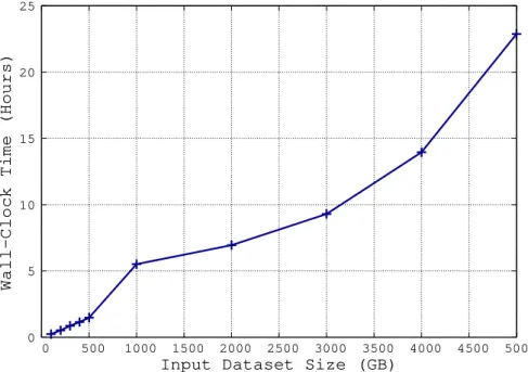
0 5 10 15 20 25 0 500 1000 1500 2000 2500 3000 3500 4000 4500 5000
Wall−Clock Time (Hours)
Input Dataset Size (GB)
Figure 3.1: Overall Execution Time for Optimisation
3.4.4
Execution Time Analysis
Figure 3.1 shows how the overall optimization time grows in relation to the input size. Table 3.1 illustrates the CPU time usage, which is useful to understand how the I/O latency contributes to the overall execution time of our data-intensive algorithm.
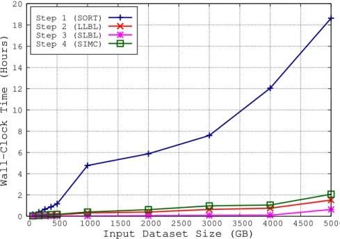
Results from both Figure 3.1 and Table 3.1 indicate two significant outcomes. Firstly, that our method is indeed capable of optimising datasets of distur-bance traces that far exceed the available amount of RAM. Secondly, that the performance decreases at a reasonable rate, whereas input data grows at a significant rate with respect to the amount of RAM used for buffering. Figure 3.2 shows how the sorting step is significantly more time-consuming than all the others. In fact, it takes as long as 12 hours to order the 4-TB
0 2 4 6 8 10 12 14 16 18 20 0 500 1000 1500 2000 2500 3000 3500 4000 4500 5000
Wall−Clock Time (Hours)
Input Dataset Size (GB)
Step 1 (SORT) Step 2 (LLBL) Step 3 (SLBL) Step 4 (SIMC)
Figure 3.2: Execution Time for each Optimisation Step
Input (GB) WC Time (sec) Usr Time (sec) Sys Time (sec) CPU Perc. (%)
100 869.96 256.97 208.19 53 200 1888.34 529.17 446.13 52 300 3123.07 807.58 728.63 49 400 4154.61 1082.31 1015.12 50 500 5330.37 1375.38 1346.83 51 1000 19860.45 2905.38 3056.02 30 2000 24998.79 6870.06 6922.10 55 3000 33479.43 9524.09 10505.79 60 4000 50248.18 12533.62 14587.52 54 5000 82325.26 17199.34 20858.58 46
3.4.5
Optimisation Effectiveness Analysis
In this section we evaluate the effectiveness of our presented optimisation method by analysing results from our benchmark. In particular, we show how much redundant simulation can be removed for each input dataset. To this end, we analyse the number of simulation intervals in both the input scenarios and the resulting simulation campaigns.
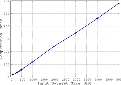
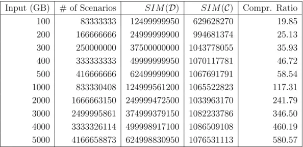
Figure 3.3 and Table 3.2 show what we call the Compression Ratio between the input datasets and the resulting optimised simulation campaigns, which we define below.
First, let SIM (D) := N · H be the number of simulation intervals in a dataset D that contains |D| = N input scenarios with horizon H. Second, letSIM (C) :=P
run(t) ∈ Ct be the number of simulation intervals in the
sim-ulation campaign C obtained from D, which is the sum of the t-arguments of run(t) commands in C. In conclusion, the Compression Ratio between the in-put dataset and the resulting optimised simulation campaign isSIM (D)/SIM (C).
0 100 200 300 400 500 600 0 500 1000 1500 2000 2500 3000 3500 4000 4500 5000 Compression Ratio
Input (GB) # of Scenarios SIM (D) SIM (C) Compr. Ratio 100 83333333 12499999950 629628270 19.85 200 166666666 24999999900 994681374 25.13 300 250000000 37500000000 1043778055 35.93 400 333333333 49999999950 1070117781 46.72 500 416666666 62499999900 1067691791 58.54 1000 833330408 124999561200 1065522823 117.31 2000 1666663150 249999472500 1033963170 241.79 3000 2499995861 374999379150 1082233786 346.50 4000 3333326114 499998917100 1086509108 460.19 5000 4166658873 624998830950 1076531113 580.57
Table 3.2: Compression Ratio per Input Dataset
3.5
Related Work
A method to compute optimised simulation campaigns from datasets of sce-narios has already been presented in [2]. The idea for this method was based on the presence of labelled lexicographically ordered datasets of in-put scenarios. In particular, it exploited such an inin-put format in order to efficiently build a Labels Branching Tree (LBT) data structure. The final simulation campaign was then computed from the LBT, which fitted entirely in RAM.
As a result, the method in [2] did not address the computation of labels, and also did not perform the ordering of input scenarios.
In contrast, the method presented in this chapter can efficiently compute simulation campaigns from large datasets of scenarios that are neither la-belled nor ordered, and that cannot be fully accommodated into the main memory.
3.6
Conclusions
In this chapter, we presented a method to increase the performance of System-Level Formal Verification (SLFV) by computing highly optimised simulation campaigns from existing datasets that contain a huge number of scenarios that do not fit entirely into the main memory.
For this purpose, we devised and implemented a data-intensive algorithm to efficiently perform the optimisation of such datasets.
In fact, results show that a 4 TB dataset of scenarios can be optimised in as little as 12 hours using just one processor with 50 GB of RAM.
Chapter 4
Execution Time Estimation of
Simulation Campaigns
4.1
Introduction
4.1.1
Framework
Simulation Based Verification (SBV) is currently the most widely used ap-proach to carry out System-Level Formal Verification (SLFV) for complex Cyber-Physical Systems (CPSs). In order to perform SBV, it is necessary to execute simulation campaigns on the CPS model to be verified.
Simulation campaigns consist of sequences of simulator commands that are aimed at reproducing all the relevant disturbance sequences (i.e., scenarios) originating from the environment in which the CPS model should operate safely.
Indeed, the goal of SLFV is to prove that the system as a whole is able to safely interact within this environment. For this reason, simulation cam-paigns include commands to inject the model with disturbances, which rep-resent exogenous events such as hardware failures and system parameter changes.
An example of a simulation campaign could have the following sequence of instructions: (i) simulate the model for 3 seconds, (ii) inject the model with a disturbance, (iii) simulate the model for other 5 seconds, and (iv) check if the state of the model violates any given requirement.
Simulation campaigns are either written by verification engineers or auto-matically generated from a formal specification model [2]. In this latter case, simulation campaigns can contain as many as 108 of simulator commands, which are stored in large binary files of up to hundreds of gigabytes.
As a result of this specification model, simulation campaigns are generated so that SLFV can be performed using an assume-guarantee approach. Namely, a successful SBV process can guarantee that the CPS will behave as expected, assuming that all and only the relevant scenarios are formally specified.
4.1.2
Motivations
Simulation campaigns necessitate a large number of simulator instructions, consequently the length of execution time required to perform SBV tends to be considerable. For example, as illustrated in [2] it takes as long as 29 days to run a middle-sized simulation campaign for the Fuel Control System model1 with one 8-core machine (see also [3][4][5]). This makes SBV an ex-tremely time-consuming process, and therefore not very cost effective. This is mitigated by involving multiple simulators working simultaneously, in the form of clusters that have hundreds of nodes and thousands of cores. For example, results in [4] show that by using 64 machines with an 8-core pro-cessor each, the SLFV activity can be completed in about 27 hours whereas a sequential approach would require more than 200 days.
However, there are still the following obstacles to effective SLFV, that in-volve the management of computing resources. In particular, clusters used to perform SBV are either controlled by commercial companies, thus subjected to strict price policies, or by community based research institutions such as the CINECA2, that offer free computation hours for research activities.
Both these kinds of clusters are typically constrained by: (i) The number of cores per task that can be used; (ii) The amount of computation hours that can be used.
As a result, it is necessary to either manage the number of cores used to reduce costs, or make the most of the limited number of free computational hours available. Furthermore, each verification phase typically has a strict deadline to be met in order to shorten the time-to-market.
An accurate execution time estimate can reveal if given deadlines can be met. If not, mitigating actions can be taken in good time. For example, the process could be limited to a subset of the simulation campaign. Another option would be to buy additional cores to execute the entire simulation campaign faster.
On top of that, a prior knowledge of the estimated execution time for a sim-ulation campaign helps in calculating the number of cores and computation hours to be bought according to the given time schedule and budget. For example, it is helpful in deciding how many slices to split the simulation campaign into according to the given constraints.
In short, an accurate estimate of execution time leads to better planning of deadlines, and wiser budget allocation for the required computing re-sources.
4.1.3
Contributions
In order to overcome the lack of tools to perform an effective estimation, we show a method that uses just a small number of execution time samples to accurately train a prediction model. In particular, we describe both how we define our prediction model, and how we choose simulator instructions to collect execution time samples.
This method brings two significant advantages.
First, that only a very small number of execution time samples are required in order to train the prediction model, thus removing the need to simulate a large simulation campaign. Consequently the estimation process is faster, and it is easier to make decisions about the number of slices to split the campaign into (i.e., how many machine to use in parallel).
Secondly, the approach we use to select which simulator commands to sample is machine-independent. Namely, decisions are made on the basis of the simulation model and the solver of the simulator. This makes it possible to select the simulator commands to train the prediction model regardless of the machine where the simulation campaign will run. As a result, we can select commands to sample only once and reuse them to train prediction models on each different machine in the cluster.
To the best of our knowledge, there are no other applicable methodologies in the literature.
4.2
Background
In this section we provide some basic definitions that will be used in the rest of the chapter.
4.2.1
Definitions
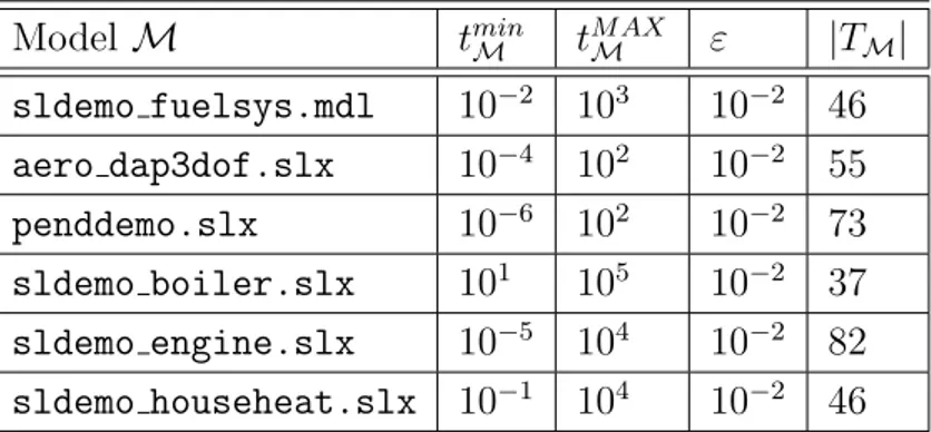
Simulation ModelDefinition 4.2.1 (Simulation Model). A simulation model (or simply model) M is a formal description of the Cyber-Physical System (CPS) to verify (e.g., the Fuel Control System3). In particular, the model is written in the language of the simulator being used.
Simulator
Definition 4.2.2 (Simulator). A simulator σ is a software tool that is able to simulate the behaviour of the given CPS model M to verify.
Set of Disturbances
Definition 4.2.3 (Set of Disturbances). A set of disturbances DM is a finite
Typically, each disturbance d ∈ DM consists in modifying some system
pa-rameters by the corresponding simulator command inject(d).
Simulation Setting
Definition 4.2.4 (Simulation Setting). A simulation setting S = (σ, M, DM, µ)
identifies the simulator σ, the model M to simulate, the set of disturbances DM to inject, and the machine µ where the simulator operates.
4.2.2
Prediction Function
Here we define prediction functions and constants used to estimate the execu-tion time of each command in a simulaexecu-tion campaign C for a given simulaexecu-tion setting S.
Function runS : N+ → R+ represents the execution time estimate of
com-mand run(t) in the setting S. Namely, runS(t) is the execution time that
the simulator takes to advance the state of the model by τ · t simulation seconds.
Constants injectS, storeS, loadS, f reeS ∈ R+ represent the execution time
estimate of commands inject, store, load, and free, in the same setting S. Based on a simulation setting S, a simulation campaign C, and a command c ∈ C, we define as follows our prediction function PS(c) to indicate the
execution time estimate for command c in the simulation setting S.
PS(c) = runS(t) c = run(t), t ∈ N+ injectS c = inject(d), d ∈ DM storeS c = store(s), s ∈ N+ loadS c = load(s), s ∈ N+ f reeS c = f ree(s), s ∈ N+
4.3
Problem Formulation
Let be given a simulation setting S and a simulation campaign C. The aim is to automatically find an accurate estimation of the execution time to simulate C in the simulation setting S by training our prediction function PS in such
a way that the resulting estimate PSC is the sum of the estimates for each simulator command c in C, i.e.,
PSC = X
c ∈ C
PS(c).
In the rest of the chapter we show how we effectively train PS and how we
validate its accuracy.
4.4
Methodology
Given how useful having an execution time estimate is, it would be tempt-ing to compute it on the basis of an existtempt-ing simulation campaign. Once collected, the execution time samples would be used to train a prediction model. However, this na¨ıve approach is risky as it could potentially lead to either poor performances or to inaccurate results for the following reasons. First, the given simulation campaign may require hours of simulations. Sec-ond, if a relatively small subset of the given campaign is used, the resulting collected samples could be either insufficient or inappropriate to train an accurate prediction model.
As an example, let us consider only the command run(t), which is the most expensive from a computational point of view. It would be natural to assume a linear relationship between the execution time erun(t) to actually simulate
it, and the number of simulation seconds τ · t that are required to advance. Namely, the estimated execution time to simulaterun(t) would be erun(t) :=
a · t + b.
To train such a simple prediction model, a careful selection of t-values to sample is needed, according to the following phenomena we observed on several Simulink models.
time grows constantly and it is strictly related to the number of numerical integration steps performed by the simulator4. Clearly, tmin and tM AX vary
depending on the complexity of the model being simulated.
Note that a typical simulation campaign includes a large number of run(t) commands with both short and long values of t. These last observations together constitute the main reason why the aforementioned na¨ıve approach would lead to inaccurate estimates, if execution time samples are not collected properly.
4.4.1
Overall Method
In order to train our prediction function PS, we use a small number of
exe-cution time samples that are sufficient to make an accurate exeexe-cution time estimate of a given simulation campaign C. To this end, we collect such samples by simulating an ad-hoc sequence C∗ of simulator commands that we choose for this purpose.
More precisely, we proceed as follows. First, we accurately choose simula-tor commands to put in C∗ in order to compute a meaningful training set. Second, we simulate C∗ to collect execution time samples in our training set. Finally, we use the resulting training set to compute parameters for our prediction function PS.
In the following sections we show how we build C∗ and more specifically which t-values we choose to collect execution time samples of run(t) com-mands.
4Simulators generally use Ordinary Differential Equations (ODE) solvers that
imple-ment state-of-the-art algorithms for numerical integration. These algorithms are designed to reduce simulation time while maintaining high numerical accuracy by dynamically choosing the integration steps to perform (https://www.mathworks.com/help/matlab/ ordinary-differential-equations.html).