Egocentric Vision Based Localization of Shopping Cart

Dipartimento di Matematica e Informatica

Dottorato di Ricerca in Matematica e Informatica XXXI Ciclo

Emiliano Spera

Egocentric Vision Based Localization of Shopping Carts

Tesi di Dottorato di Ricerca

Prof. Giovanni Maria Farinella

Abstract

Indoor camera localization from egocentric images is a challenge computer vision problem which has been strongly investigated in the last years. Localizing a camera in a 3D space can open many useful applications in different domains. In this work, we analyse this challenge to localize shopping cart in stores. Three main contributions are given with this thesis. As first, we propose a new dataset for shopping cart localization which includes both RGB and depth images together with the 3-DOF data corresponding to the cart position and orientation in the store. The dataset is also labelled with respect to 16 different classes associated to different areas of the considered retail. A second contribution is related to a benchmark study where different methods are compared for both, cart pose estimation and retail area classification. Last contribution is related to the computational analysis of the considered approaches.

Acknowledgements

I would like to tanks my supervisor Prof. Giovanni Maria Farinella as well as Prof. Sebastiano Battiato and Dr. Antonino Furnari for their guide and support during my PHD studies.

Contents

Abstract ii

Acknowledgements iii

1 Introduction 1

1.1 Motivation . . . 1

1.2 Aims and approaches . . . 2

1.3 Contributions . . . 4

2 Related Works 7 2.1 Localization in a retail store . . . 7

2.2 Image based camera localization methods . . . 7

2.2.1 Classification based methods . . . 8

2.2.2 Regression based approaches . . . 8

2.3 Dataset . . . 10

3 Background 12 3.1 Structure from motion . . . 12

3.1.1 Features and matching . . . 13

3.1.2 Camera pose estimation . . . 13

3.1.3 3D structure estimation . . . 14

3.1.4 SAMANTHA . . . 18

3.2 Support Vector Regression . . . 20

3.3 K-NN regression . . . 24

3.4 Improved Fisher Vector . . . 24

3.5 Siamese and Triplet networks . . . 25

4 EgoCart dataset 30 4.0.1 3-DOF labels . . . 31

4.0.2 Classification labels . . . 34

4.0.3 Error analysis . . . 35

5 Methods 39 5.1 Image retrieval methods . . . 39

5.2 Regression based methods . . . 41

5.3 Classification methods . . . 46

5.4 Depth . . . 47

5.4.1 3 DOF camera pose estimation . . . 47

5.4.2 Classification . . . 47

5.5 Experimental settings . . . 48

6 Results 50 6.0.1 Retrieval based methods . . . 50

6.0.2 Regression based methods . . . 55

6.0.3 Retrieval based methods VS Regression based methods . . . . 60

6.0.4 Classification . . . 62

7 Conclusion and future works 66 A 68 A.1 Other Publications . . . 68

Chapter 1

Introduction

1.1

Motivation

The ability to estimate the position and orientation of a mobile object from egocen-tric images is crucial for many industrial applications[14, 11, 13]. In robotics, for instance, the opportunity to use a camera for the auto-localization of the robots is a cheap solution and not invasive for the context. In outdoor contexts the more tradi-tional technology used for localization is the GPS, differently the classic solutions to address indoor localization include the employment of RF-ID tags [1] or Beacons [2] and the use of fixed cameras monitoring the different areas of the indoor context [4]. While these technologies can be used to obtain effective localization systems, they both have downsides. For instance, GPS and Beacons are not very accurate [2] and struggle with occlusions which can attenuate their signal [3], whereas pipelines based on fixed cameras need the installation of camera networks and the use of complex algorithms capable of re-identifying people across the different scenes.

To overcome these issues, localization using egocentric images has been investi-gated both in the context of indoor and outdoor environments [11, 13, 14] according to different levels of localization precision, in function of the environment character-istics and of application in which is involved, e.g. 6 Degrees Of Freedom (6-DOF) pose estimation [11, 13] for 3D location estimation, 3-DOF pose estimation [9] for 2D location estimation and room-based location recognition [22, 40, 41].

As it has been investigated by Santarcangelo et al. [40], in the context of retail stores, the position of shopping carts equipped with a camera can be obtained exploiting computer vision pipelines for scene classification. Such information can be used to analyse the customer behaviours, trying to infer, for instance, where they

spend more time, which areas of the store are preferred (e.g., fruit, gastronomy, etc.) and how the placement of products can affect sales. Image-based localization abilities are also necessary to allow a robot to navigate and monitor the store or to assist the costumers [21].

1.2

Aims and approaches

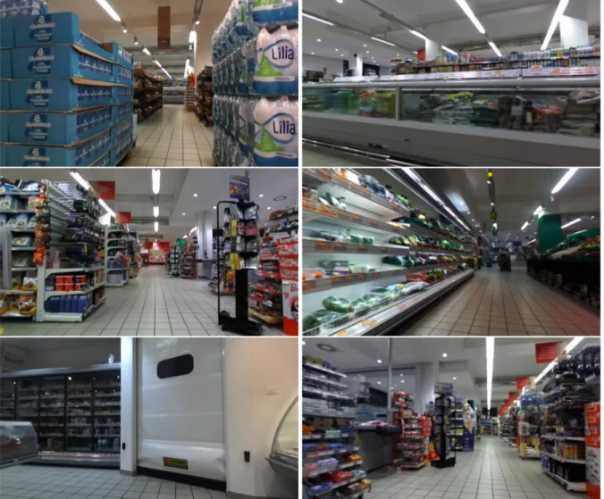
This thesis work is focused on the problem of localizing shopping carts in retail stores from egocentric images acquired by cameras mounted on shopping carts. Differently from other indoor environments, retail is a very hard and specific environment for camera localization presenting unique properties and challenges:

• It is often large scale environment

• The 3D structures are typically repetitive (e.g. many shelves with same di-mensions)

• similar products, form a visual point of view, can be in different parts of the store

• many visually dissimilar products are spatial near producing a strong visual difference between images acquired in similar position.

Figure 1.1 shows some examples of the typical variability of egocentric images ac-quired in a retail store.

In the last years the growing interest related to localization by means of egocen-tric images bring the scientific community to produce different dataset to address this task in indoor and outdoor environment [11, 14, 13]. Despite this growing in-terest a large dataset to address the task of shopping cart localization in a retail store was still missing. Hence, during my PHD activity, we proposed a new large scale dataset of RGB and depth images acquired in a retail store by using cameras mounted on shopping carts. By means of careful semi-automatic 3D reconstruction and registration procedures, each image has been labelled with a six Degrees Of Freedom (6-DOF) pose summarizing the 3D position of the shopping cart, as well as its orientation in the 3D space.

Our data analysis points out that most of the variance of the collected shopping cart positions is explained by their first two principal components. This leads us to frame the egocentric shopping cart localization problem as a three Degrees Of Freedom (3-DOF) pose estimation task. Therefore, we created a 3-DOF version of the dataset by projecting the 6-DOF poses onto a 2D plane parallel to the floor of the store. In this version of the dataset, each frame is associated with the 2D coordinates and angle describing the position and orientation of the shopping cart. Furthermore, to allow a deeper analysis of the problem, for each image of the dataset we furnished a depth image and a belonging class. The dataset was divided in 16 different classes each of them groups all the images of a convex area of the store. We decided to introduce depth image informations to analyse their usefulness to pose prediction and because several devices available on the market are now able to provide it in real time1_.

In order to deep investigate cart localization problem we benchmark two principal classes of approaches based on classification and regression.

The camera 3-DOF regression problem was investigate through two different families of methods:

• Traditional image retrieval based approaches • Camera 3-DOF regressor-based approaches

Moreover an analysis of how much depth images can be useful to improve regres-sion and classification performances was proposed. To examine which techniques shall be preferred depending on the computational constraints imposed by the em-ployed hardware and by real-time requirements we proposed also a computational comparison of the different approaches.

1.3

Contributions

The main contributions of this thesis are the follow: 1_{http:www.stereolabs.com}

• We propose a dataset to study the problem of egocentric shopping cart local-ization as classification and regression problem. The dataset is intended to foster research on the problem and it is publicly available at our web page2_; • We benchmark classification, retrieval-based and regression-based localization

techniques in the proposed application domain

• We propose an analysis of time performance and memory usage of best ap-proaches

• We investigate different loss functions and architectures for CNN-based ap-proaches

• We study the usefulness of depth information for classification and regression task in the considered context

The principal contribution of this thesis have been published in international journal and conferences:

International journal :

• E. Spera, A.Furnari, S. Battiato and G.M.Farinella. Egocart: shopping cart localization from egocentric videos.Submitted to Computer Vision and Image Understanding

International conferences:

• E.Spera,A.Furnari,S.Battiato,G.M.Farinella. Egocentric Shopping Cart Lo-calization. In International Conference on Pattern Recognition (ICPR), 2018 • E.Spera,A.Furnari,S.Battiato,G.M.Farinella.Performance Comparison of

Meth-ods Based on Image Retrieval and Direct Regression for Egocentric Shopping Cart Localization. In 4th International Forum on Research and Technologies for Society and Industry (RTSI), 2018

Appendix A reports a list of other works not directly related to this thesis published during my Ph.D.

The remainder of this work is organized as follows: In Section 2, we review the state of the art approaches for camera localization. In Section 3, we review the prin-cipal classic methods that we used during our study. In Section 4, we present the proposed shopping chart localization dataset. Section 5 discusses the approaches in-vestigated in this study, whereas Section 6 discusses the results. Section 7 concludes the paper and reports insights for future research.

Chapter 2

Related Works

2.1

Localization in a retail store

Previous works have investigated the problem of localizing customers in a retail store. For instance, Contigiani et al. [5] designed a tracking system to localize cus-tomers using Ultra-Wide Band antennas installed in the store and tags placed on the shopping carts. Pierdicca et al. [6] addressed indoor localization using wire-less embedded systems. Other researchers has focused on the integration of vision and radio signals to improve localization accuracy. Among those, Sturari et al. [2] proposed to fuse active radio beacon signals and RGBD data to localize and track customers in a retail store. Other researchers focused on computer vision based solutions. Liciotti et al. [7] used RGB-D cameras to monitor customers in a retail environment. Del Pizzo et al. [8] designed a system to count people from RGBD cameras mounted on the ceiling.

Differently from the aforementioned works, we consider a scenario in which shop-ping carts are localized relying only on images acquired from an on-board egocentric camera.

By the point of view of our research the localization of the shopping cart can be see as the camera localization task.

2.2

Image based camera localization methods

Camera localization methods are divisible in two principal families: algorithms that face the task as a classification problem and others that treat it as a regression prob-lem. The regressive approaches are divided in two principal subfamilies: methods

based on image-retrieval and methods based on regressors.

In this section we propose an overview of works related to these different approaches.

2.2.1

Classification based methods

Classification-based approaches [22, 40, 41, 56, 54] face localization problem in a space divided in different areas and, by dividing the dataset in classes related to the different areas, tackle localization as classification problem.

These approaches aren’t able to produce a fine-grade position estimation (e.g., ac-curate 2D or 3D coordinates) but could be the best choice in context in which a fine-grade estimation is not useful or is too hard to have.

Some of these methods are based on a BoW representation [56, 54]; differently in [41] transfer learning techniques and an entropy-based rejection algorithm have been used to employ representations based on Convolutional Neural Networks (CNN). On the other hand in [22] a CNN is trained end to end to face image geolocation problem as a classification-problem. They subdivide the surface of the earth into thousands of multi-scale geographic cells and show how their classification network outperforms classical approaches based on image-retrieval. Different classification methods [75, 76, 77, 78] use dataset of landmark building obtained through the clustering of web-photo collection. These methods normally lever on the landmark building framed to perform image retrieval approaches. Differently in [79] Support Vector Machine was trained on BoW of the different clusters associated with the landmark buildings. In Grocery context Santarcangelo et al. [40] propose a hierar-chical classifier of egocentric image from a shopping cart that jointly classify action of the cart (stop and moving) and market department (e.g. Fruit,Gastronomy).

2.2.2

Regression based approaches

Unlike the classification approaches, regressive approaches try to predict accurately the 6-DOF camera pose starting by acquired image. Some of these methods are based on image retrieval techniques [46, 47]; they work by associating to a query image a set composed by the more similar images of geo-tagged training set in a particular features space and defined a specific metric. Different heuristics (e.g., k-NN approach) are finally used to estimate query image pose starting by the poses

of images included in the set associated to it. Over the years, to improve these methodologies, some study focused on confusing [50] and repetitive [51] structures, or to scale to larger scenes [49], [52]. To handle large datasets, image retrieval meth-ods that take advantage of descriptor quantization, inverted file scoring, and fast spatial matching, were proposed [45] [48] [46].

The image representation has a central role in image retrieval approaches. Some approaches encode the images using hand-crafted local features [23, 24], other use features extracted from CNNs intermediate layer. Some works use representation extracted from CNN model trained on different dataset on other task [26], other methods use representation extracted from CNN trained using the target dataset on classification or regression [28].

In [53], in order to face with the disturbing presence of repetitive structures, an automatically weight of features on the similarity score between images is proposed to reduce the impact of those related to repetitive structures and to take more the features with an unique local appearance into account.

Also Triplet and Siamese networks have been used to learn the features to address the 3D object pose estimation [32, 33], a task strongly correlated to that we are investigating in this work. In some of these works a contrastive loss [29] was used to train the network to build a features space in which similar images result clustered and dissimilar images result faraway between them [30, 31]. Some works investigate camera pose estimation in shopping small. In [81] the authors propose a methods based on Markov Random Field that, using monocular images and the shopping mall’s floor-plan, jointly perform text detection, shop facades segmentation and camera pose estimation. In [80] was proposed a method based on two consecutive steps. In the first step the query image is matched by involving matching of store signs with the training set images to identify the ”closest”. In the second step the pose of the query image, respect to the ”closest” camera reference system, is com-puted. Many of regression-based methods are based on a 3D model of the scene [14] [15] [37]. Associating the 3D points with one or more local descriptor, these methods build a matching between local features extracted by query image and a set of 3D points. Starting by these 2D-3D matching a query image pose is estimated using different heuristics [38] [39] [43]. To solve the time consuming problem, procured by descriptor matching task, different strategies were proposed: either searching for

the match on a subset of the 3D points [44], or based on a 3D model compression scheme [55, 79].

In the last years many works investigate CNN-based approaches that try to regress camera pose directly from images. In [11] the first end-to-end CNN based model for pose regression (POSENET) was proposed. This model based on GoogleNet architecture [42] has been obtained replacing classification layers with two fully connected layers to tackle the regression task. In [12] two different loss functions were proposed for the same architecture: one is based on trying to learn an opti-mal balance between position error and orientation error, the other one is based on geometric re-projection error. In [13] Long-Short-Term-Memory (LSTM) was combined with Posenet architecture for camera pose regression. The LSTM units allow to identify a more useful feature’s correlations for the task of pose estimation. In [57] the authors use encoder-decoder CNN to camera pose prediction. In [58] a multi-task CNN, to deal the trade-off between orientation and position, and a data augmentation method for camera pose estimation was proposed. Even if these meth-ods result less performing, in term of accuracy, compared to the methmeth-ods based on 3D models, they are characterized by compactness and very short processing times. These characteristics make this family of methods very likable, in particular for work in embedded settings.

2.3

Dataset

In the last years different datasets were proposed in indoor and outdoor environments for camera localization task. One of the best known, for indoor context, is 7-Scenes dataset. This dataset was released in 2013 by Microsoft and formed by 7 different scenes and for each scene several sequences were provided each one consisting of 500-1000 frames. The dataset was collected using a handheld kinect RGB-D camera at 640 × 480 resolution. To obtain ground truth cameras poses, an implementation of the KinectFusion system and a dense 3D model of the scenes were used. The dataset was built extracting frames from different sequences for each scene. Each frame is formed by RGB images, depth images and positions and orientations of the cameras. Like most indoor datasets, in 7 scene dataset as well,the scenes are spanning the extension of a single room, only in the last years large scale indoor

dataset was proposed. In [13], for instance, the authors propose TU Munich Large-Scale Indoor dataset and it is one of the first covering a whole building floor with a total area of 5,575 m2_{. In order to generate ground truth pose information for} each image, the authors captured the data using a mobile system equipped with six cameras and three laser range finders. In [82] a dataset acquired in the ground level of a shopping mall with an extenction of 5,000 m2 _{was proposed. The training set} images of this dataset was captured using DSLR cameras while test set is composed by 2,000 cell phone photos taken by different users. To estimate ground truth camera pose 3D-2D matching algorithm was used levering on a 3D model obtained with a high precision LiDAR scanner.

Related to outdoor context, relevant datasets are Rome16k and Dubrovnik6k [79], and The Cambridge Landmarks dataset in [11]. Dubrovnik6k and Rome16k datasets were build from photos retrieved by Flick, the first is formed by 6,844 images while the second by 16,179 images. Both these datasets contain also 3D model of the scenes. The Cambridge Landmarks dataset is formed by 5 different scenes and contains 12K images with full 6-DoF camera poses. All these three outdoor datasets were generated using Structure From Motion algorithm.

In grocery context only VMBA15 dataset [40] composed by 7839 samples is available, the images are labelled according to action (i.e. stop, moving) location (indoor, outdoor) and scenes context (e.g. gastronomy, fruit) but isn’t labelled in terms of 6 D.O.F. of the cameras.

Chapter 3

Background

3.1

Structure from motion

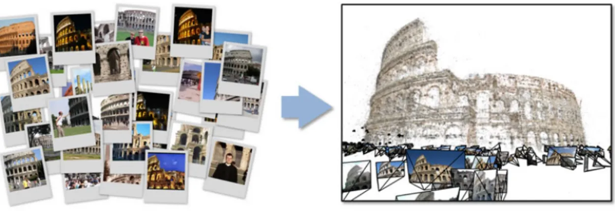
Starting from a set of images acquired in the same scene, Structure From Motion (SFM) problem consist by recovering the 3D scene and the camera 6 DOF for each image of the set.

Figure 3.1: Structure From Motion aim1

The SFM algorithms are based on three main stage:

• By extracting image features and matching the features extracted by different frames between them

• Estimation of camera motion

• By buildind the 3D scene using the estimated motion and features 1

3.1.1

Features and matching

Different features were proposed for SFM task. One of the most used features is the scale invariant feature transform (SIFT) [64], which has been extensively used in many of the SFM methods based on corresponding point. The SIFT features, based on local gradient histograms, result to be well performing for SMF methods because of their invariant to scaling and rotation, and their robustness as it regards illumination changes. To obtain a more compact representation in [65] PCA-SIFT features were proposed, obtained by applying principal component analysis (PCA) to the image gradients. Others features largely used in SFM algorithms are Speeded-Up Robust Features (SURF) as proposed in [66]. These features are invariant respect to scale and rotation as well and they require less computational cost for extraction compared with SIFT features. The features matching is generally performed by considering similar descriptors to be more likely matches. In many cases match correctly the features extracted by different images is a very hard task. For instance the presence in the 3D space of different objects that look similar can produce incorrect match of unrelated features and consequently major errors in camera pose estimation and 3D reconstruction. To face with ambiguity problem during features matching, different disambiguation approaches were proposed. In [67] the incorrect features matches are identified by means of relations induced by pairwise geometric transformations. Differently, in [68] disambiguation is performed by optimizing a measure of missing image projections of potential 3D structures.

3.1.2

Camera pose estimation

The first works, which investigate the theoretical opportunity to estimate camera pose using matching points, are of the early twentieth century. In [69] was proved for the first time that given two images, both framing at least the same five distinct 3D points, is possible to recover the positions of the points in the 3D space and at the same time the relative positions and orientations between the cameras up to a scale value. After many years by this first work, in [70] was showed that it’s possible to estimate essential matrix of two cameras starting from eight different points correspondents just solving a linear equation. They also showed that, by mean of the decomposition of the essential matrix, is possible to obtain the relative

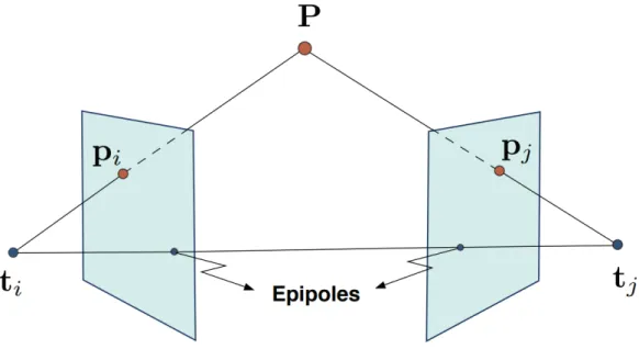
cameras orientations and positions. The basic idea for the position and orientation camera estimation is levering on the epipolar constraints Eq. 3.1 imposed by the points matching by using the pinhole camera model (Figure 3.2).

pT_i ([R_iT(tj − ti)]×R_iTRj)pj =: pTi Eijpj = 0 (3.1) where pi and pj are the representation of the 3D point P respectively on the image planes i and j. ti and tj are the locations and Ri and Rj the orientation matrices respectively of the i’th and j’th camera and Eij ∈ R3×3 is the essential matrix

Figure 3.2: Pinhole camera model2

It’s easy to observe that fixing a scale for the entries of Eij (e.g. ∥Eij∥ = 1) the 9 different elements of the essential matrix can be determined just imposing eight points matches and consequently eight epipolar constraints.

3.1.3

3D structure estimation

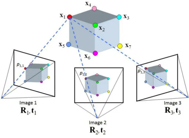
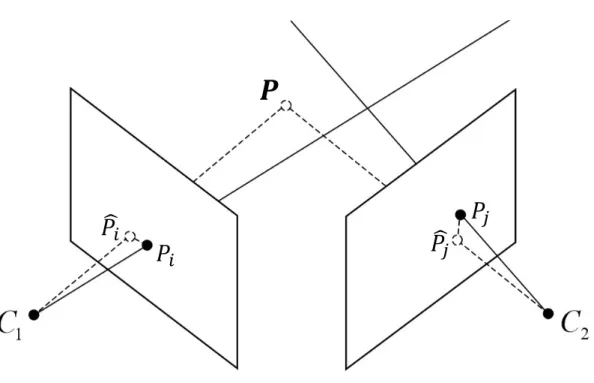
The methods for 3D points estimation are classically based on triangulation (Fig-ure 3.3). Given the projection matrices of different cameras is theoretically possible

to compute the exact 3D points position in the scene from their positions in images acquired by two or more views. Because of the noise, the back-projected rays, start-ing by the different centres of projection of cameras, are not generally intersected each other.

Figure 3.3: Graphical representation of triangulation procedure 3

To find a good approximation of the 3D points locations, several methods try to minimize an appropriate error metric. Given a 3D point, the standard reconstruction algorithm identifies the 3D coordinate of the point as those that minimize the sum of squared errors between the measured pixels positions associated to the 3D point in two or more images, and the theoretical pixels positions associated to the 3D

point, on the same images, computed by mean of projections Eq.3.2 P = arg min P ∑ i=1 ∥pi− ˆpi(P )∥2 (3.2)

Where P is the predicted 3D point, piis the measured pixel position associated to 3D point in the i’th image and ˆpi(P ) is the predicted pixel position for the same view (Figure 3.4). If the pixels positions noise is Gaussian-distributed this optimization give the maximum likelihood solution for P.

Figure 3.4: Graphical representation of minimization of the squared errors sum between measured and predicted pixel positions during triangulation

To face with SFM problem for an arbitrary number of view, two different ap-proaches types were proposed: the sequential and the factorization algorithms. The sequential approaches are those working adding a different view one at time to the scene. These algorithms typically produce a scene initialization by computing cam-era orientation and 3D points cloud for the first two views. For any other image

added to the scene a partial reconstruction is performed, by computing the positions of 3D points through triangulation. Different approaches were used to register new views to the scene, some of them levering on the two-view epipolar geometry to esti-mate position and orientation of the new camera starting by those of its predecessor. Other methods use the 3D-2D correspondents between the already reconstructed 3D points and the features extracted from the new image to determine its pose. In fact, it is possible to prove that through only 6 3D-2D matches the camera pose can be determinate. Other sequential SFM algorithms work by merging partial reconstruc-tions related to different subset of views by using 3D points correspondents.

Differently from sequential approaches, factorization methods work computing 3D points cloud and cameras poses by using all the images simultaneously. This family of methods, introduced in [71], is generally based on direct SVD factorization of a measurement matrix composed by the measurements of the 3D points by the dif-ferent cameras. These algorithms, compared to sequential methods, achieve a more evenly distributed reconstruction error across all measurements, but they fail for some structure and motion configuration.

Obtained a initial estimation of 3D points and of cameras poses a refinement pro-cess of these estimations are usually conducted using bundle adjustment techniques. Bundle adjustment works with an iterative non linear optimization to minimize a cost function related to a weighted sum of squared re-projection errors.

Bundle adjustment procedures try to determine an optimal set of parameters δ not directly measurable (cameras projection matrices, 3D points coordinates) for a set of noisy observations (e.g. pixel position associated to 3D points). Given a set of measurements Mi and the set of δ-dependent associated estimations, the features prediction errors Mi(δ) are defined as:

∆Mi(δ) =: Mi− Mi(δ) (3.3)

Bundle adjustment produces a minimization of a cost function depending of the likelihood of the features prediction errors. Assuming a Gaussian-distribution of the noise associated with the measurements, a typical appropriate cost function is:

f (δ) = 1 2

∑

i

where Wi is the matrix that approximate the inverse covariance matrix of the noise associated with the measurement Mi. To optimize the cost function during bundle adjustment procedure several optimization methods were used and three main categories were strongly investigated during the years:

• the second-order Newton-style methods • first order methods

• the sequential methods incorporating a series of observations one-by-one A deep analysis of these methods was proposed in [72].

3.1.4

SAMANTHA

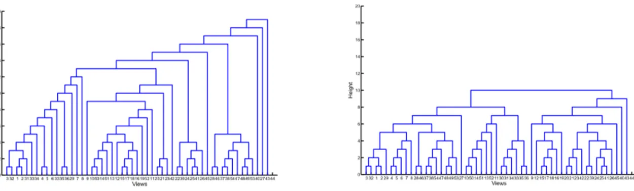
In this section we will describe the SFM algorithm [17, 16] used to obtain poses labels for the images of our dataset. This algorithm is based on a reconstruction process levering on a binary tree built through a hierarchical cluster of the images set. Each image corresponds to a leaf of the tree while the internal nodes are as-sociated to a partial reconstruction of the model obtained by merging the partial models associated to the two sub-nodes. The first step of SAMANTHA algorithm is to perform the extraction of features based on difference of Gaussian with radial descriptor. The features matching is performed using nearest neighbour approach and different heuristics are sequentially implemented to maintain only the more sig-nificant matches. Given the features matching, an image affinity measure is used, in agglomerative clustering algorithm, to build the hierarchical cluster tree. The im-age affinity measure used takes in account the number of features matching between images and how much the features are spread in the images. With a bottom-up procedure the agglomerative clustering algorithm, starting from clusters formed by single images, merge iteratively the clusters with the smallest cardinality (sum of the views belonging to the two clusters) among the n closest pairs of clusters. The simple linkage rule is used to measure the distance between the different clusters. By exploiting the cardinality of the clusters during agglomerative clustering pro-cedure, the algorithm is able to produce a more balancing hierarchical cluster tree (Figure 3.5) and consequently a reduction of time complexity [16].

Figure 3.5: Example of hierarchical cluster tree produced merging the closest clusters using simple linkage role (left) and the more balanced tree obtained merging the clusters

with the smallest cardinality among the n closest pairs4

Computed this hierarchical organization of the images the scene reconstruction is implemented. During this process three different operations are involved: the two views reconstruction ( to merge two different views), a resection-intersection step to add a single view to the model and the fusion of two partial models (Figure 3.6).

Figure 3.6: Example of hierarchical cluster tree in which on each internal node is associated the relative reconstruction operation. The circle corresponds to the creation of a stereo-model, the triangle corresponds to a resection-intersection, the diamond corresponds to a

fusion of two partial independent models. 5

3.2

Support Vector Regression

The Support Vector Regression is a generalization of Support Vector Machine for regression task. Suppose to have a training set (x1, y1), (x2, y2), ....(xn, yn), with xi ∈ X where X denotes the space of the input patterns and yi ∈ R, the Support Vector Regression method try to find a function f (x) that have at most a distance ϵ from all the target yi and is as flat as possible. This method therefore do not care about errors smaller than ϵ and optimize the parameters of f (x) considering the prediction error bigger than ϵ. In this algorithm a central role is played by the choice of f (x) function (e.g. linear, Polynomial). By using a linear function Eq.3.5

f (x) = ⟨w, x⟩ + b (3.5)

with w ∈ X and b ∈ R is possible to write the regression problem as the minimization problem of the Soft Margin Loss functon Eq.3.6 [63]

minimize 1 2∥w∥ 2 _{+ C} n ∑ 1 (δi+ δi∗) (3.6)

subject to the follow constraints:

yi− ⟨w, xi⟩ − b 6 ϵ + δi ⟨w, xi⟩ + b − yi 6 ϵ + δi∗ δi, δi∗ > 0

(3.7)

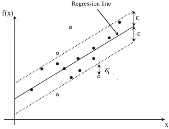
where δi and δ∗i are variables that represent how much the target i is far from the area around the regression function, identified by the margin ϵ (Figure 3.7). The variables aforementioned are defined as follows:

δϵ := {

0 if _{δ 6 ϵ}

∥δ − ϵ∥ otherwise (3.8)

where δ =∥yi− f (xi)∥, δi = δϵ if yi > f (xi) and δ∗i = δϵ otherwise.

The constant C > 0 in 3.6, fixes a trade-off between the flatness of f and the amount of tolerated deviations larger than ϵ.

𝒊 ∗

Figure 3.7: Soft margin loss for linear SVR

The minimization problem 3.6 can be solved using its dual formulation obtained through the Lagrangian function L:

L := 1 2∥w∥ 2_{+ C} n ∑ i=1 (δi+ δ∗i) − n ∑ i=1 (ηiδi+ η∗iδ ∗ i)+ − n ∑ i=1 αi(ϵ + δi− yi+ ⟨w, xi⟩ + b)+ − n ∑ i=1 α∗_i(ϵ + δ∗_i + yi − ⟨w, xi⟩ − b) (3.9)

where the Lagrange multipliers αi, αi∗, ηi and ηi∗ have to satisfy the follow con-straint:

αi, α∗i, ηi, η∗i > 0 (3.10) Imposing equal to zero the partial derivatives of L, with respect to the primal variables (w, b,....), it’s possible rewrite the equation 3.9 as the follow dual optimiza-tion problem: maximize ⎧ ⎪ ⎪ ⎨ ⎪ ⎪ ⎩ −1 2 n ∑ i,j=1 (αi − α∗i)(αj− α∗j)⟨xi, xj⟩ −ϵ n ∑ i=1 (αi+ α∗i) + n ∑ i=1 yi(αi+ α∗i) (3.11) subjected to: n ∑ i=1 (αi− α∗i) = 0 and αi, α∗i ∈ [0, C] (3.12) by levering the conditions imposed on partial derivatives the function f (x) can be expressed as follow: f (x) = n ∑ i=1 (αi− αi∗)⟨xi, x⟩ + b (3.13)

This formulation allows to evaluate f (x) in terms of dot products between the data without compute explicitly w. Different optimization methods can be used to compute the b variable (e.g. using KKT conditions, interior point optimization method).

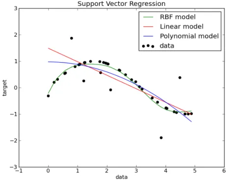
The typical approach to make SVR algorithm able to regress a non linear function consist to map the input onto a m-dimensional features space, by using some fixed (non linear) mapping, and then by applying the standard SVR algorithm to build a linear model in this feature space. Fixed a mapping function γ and defined the Kernel function K as dot product in the mapping space:

the linear regressive function in the feature space can be expressed as folow: f (x) = n ∑ i=1 (αi− αi∗)K(xi, x) + b (3.15)

Some of the kernel functions most commonly used are the Polynomial function Eq.3.16 and the Radial basis function Eq.3.17

K(x, xi) = (⟨γ(x), γ(xi)⟩ + C)d (3.16) K(x, xi) = exp ( − ∥x − xi∥ 2 2σ2 ) (3.17) Where d is the degree of the polynomial while σ is a free parameter.

As can be observed in Figure 3.8 the ability of SVR algorithm to perform a good regression strongly depend on the kernel function used.

Figure 3.8: Sample of SVR regression curve obtained with different kernel on toy 1D data.6

6_{image by http://scikit-learn.org/stable/auto_examples/svm/plot_svm_regression.}

3.3

K-NN regression

K nearest neighbours is a simple and classical algorithm for the variable’s regression. Given a query example and fixed a value of K, the basic idea of K-NN approach is to associate to the query example the average of the K nearest neighbours examples in the representation space. The average can be weighted with a multiplicative factor inversely proportional to the distance between query example and neighbours in the representation space. The choice of the distance used and of the K value have a central role for the algorithm performance. Classically, euclidean, cosine or Manhattan distances have been largely used for K-NN approach. The K value choice is frequently done through cross validation approach.

3.4

Improved Fisher Vector

Fisher Vector [19] is a global image descriptor obtained by pooling local image features. It works capturing the average of the differences, of first and second order, between the images descriptors and the centres of the Gaussian Mixed Model (GMM) that fits the distribution of the descriptors of the whole dataset. This representation was strongly used for image classification task. The procedure to build a Fisher Vector representation consist of different phases:

• extract a set of descriptors ⃗x1,...,⃗xN (e.g. sift) from each image • learn a GMM fitting the distribution of the descriptors

• compute a soft assignments of each descriptor xi to the K Gaussian compo-nents given by the posterior probability:

qik = exp[−1/2(⃗xi− ⃗µk)T ∑ −1 k (⃗xi− ⃗µk)] K ∑ 1 exp[−1/2(⃗xi− ⃗µk)T ∑ −1 k (⃗xi− ⃗µk)] (3.18)

• given the set of descriptors x1,...,xN of an image, for each k=1,...,K, compute the mean and variance deviation vectors

ujk = 1 N√πk N ∑ i=1 qik xji− µj,i δjk (3.19) vjk = 1 N√2πk N ∑ i=1 qik [( x_ji− µj,i δjk )2 − 1 ] (3.20)

• build Fisher vector for the query image as concatenation of uk and vk for all GMM components:

F V = [⃗u1, ⃗v1, ..., ⃗uk, ⃗vk] (3.21) The Improved Fisher Vector add other two components to classical Fisher Vector: the use Helling’s kernel (or other non-linear additive kernel) and the normalization of the Fiher Vector through the l2 _{norm. A modified version of Improved Fisher} Vector is the spatially enhanced Improved Fisher Vector, it is obtained appending to the local descriptors ⃗xi their normalised spatial coordinates (wi, hi) in the image before the quantization with the GMM as show below:

⃗ xSE_i = [ ⃗xT_i ,wi W − 0.5, hi H − 0.5 ]T (3.22) where W × H are the dimensions of the image.

3.5

Siamese and Triplet networks

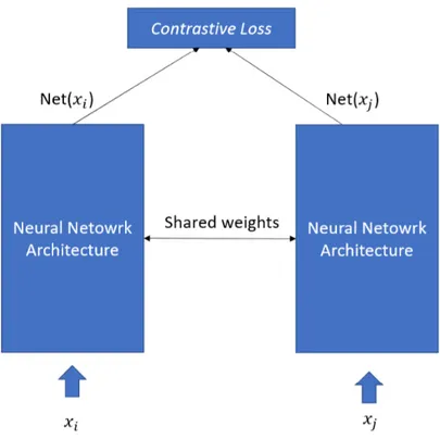
In the last years Siamese and Triplet architecture was used in computer vision for different tasks as classification or 3D object pose estimation. A Siamese network consist of two networks, sharing the same weights, that are trained with couple of images labelled as similar or dissimilar. This type of network (Figure 3.9) can be trained with contrastive loss Eq.3.23 on embedding space with the aim to minimize

Figure 3.9: Typical siamese network architecture using contrastive loss

distance between similar samples and maximize distance between dissimilar images in the representation space.

Contrastive Loss() = 1/2 ∗ δ(yi, yj) ∗ (∥N et(xi) − N et(xj)∥2)+ +1/2 ∗ (1 − δ(yi, yj)) ∗ (∥N et(xi) − N et(xj)∥2)

(3.23)

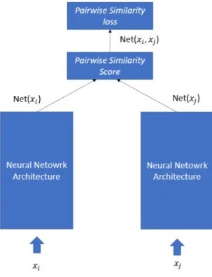
Where δ(.) denotes the Dirac delta function, yi and yj are the labels associated to the frame xi and xj, N et(x) is the embedding representation space produced by the network for the image x. Another typical loss function used to train Siamese network is the pairwise similarity loss:

P airwise Similarity Loss() = δ(yi, yj) ∗ (1/k + N et(xi, xj))+ +(1 − δ(yi, yj)) ∗ N et(xi, xj)

(3.24)

Figure 3.10: Typical siamese network architecture using pairwise similarity loss

The Siamese networks has been extended as triplet networks formed by 3 in-stances of the same feedforward network with shared parameters (Figure 3.11). This architecture during training take 3 input images, an anchor image denoted with x, a positive sample similar to the anchor sample denoted with x+ _{and a negative} sam-ple dissimilar to the anchor samsam-ple denoted with x−. When fed with the samples, the network outputs the distances between anchor sample representation and the representations of positive and negative samples in the embedding space.

This architecture is typically trained to separate similar samples by dissimilar in embedding space of a margin m (Figure 3.12) using the following Triplet loss Eq.3.25:

T ripletLoss() = max(d(N et(x+), N et(x)) − d(N et(x−), N et(x)) + m, 0) (3.25) where d is a distance defined in embedding space.

Neural Network Architecture 𝑥 Neural Network Architecture 𝑑 𝑁𝑒𝑡 𝑥 , 𝑁𝑒𝑡 𝑥 𝑁𝑒𝑡(𝑥 ) Shared weights Triplet loss Neural Network Architecture Shared weights 𝑥 𝑥 𝑁𝑒𝑡(𝑥) 𝑁𝑒𝑡(𝑥 ) 𝑑 𝑁𝑒𝑡 𝑥 , 𝑁𝑒𝑡 𝑥

Figure 3.11: Typical siamese network architecture using pairwise similarity loss

by using typical Siamese and Triplet losses, most of the pairs or triplets samples produce a small or non-existent networks weights update during the training. Due to these two undesirable characteristics a huge number of pairs or triplets of sam-ples must be processed to obtain a robust model. Moreover, sampling all possible pairs or triplets, as the size of the training dataset increases, can quickly become intractable and produce very slow convergence of the models. To face with this sampling problem, different heuristics was proposed in the last years. Some works prose a smart sampling strategy [59], by selecting pairs or triplet samples to avoid the useless samples for the training and to focus on the samples that show the most contradictory representations. Other works attach the problem by proposing global loss function to train the network [60] .

Distance Pull Push Anchor Positive sample Negative sample

Chapter 4

EgoCart dataset

In this section we introduce a large-scale indoor dataset of geo-localized images in grocery context proposed to address the shopping cart localization problem through egocentric images. Usually to build an accurate dataset for camera localization task, using only cameras, is necessary to acquire a huge quantity of images (normally through the acquisition of continuous videos) and, using SFM algorithms, infer at the same time a 3D model and image poses [11]. The images are in this way labelled with 6-DOF camera poses using 3D coordinates for the positions labelling and quaternions, Euler angles or other angular representation [58] for the camera orientations. In accordance with [13], we observe how this procedure become very difficult to apply in the context we are analysing, due to two principal reasons:

• The presence of repetitive structure elements (e.g, shelves, products, doors, check-out) that tend to create ambiguity.

• The big dimension of the environment that implies the need of a big number of images, and consequently a high computational cost, to build an accurate 3d model and an accurate poses estimation.

The datasets proposed for camera localization in indoor context are mostly re-lated to small space with extension of a single room and only few dataset was proposed for camera localization in large scale indoor environments. For the com-plexity to apply standard procedure to build this type of dataset in large scale indoor environments, some time other sensors were used to simplify the dataset collection. In [13], for instance, the dataset was collected using a system composed by six high resolution cameras and three laser range finders.

To address the hard task of build a dataset for camera localization in our setting and to maintain a lower computational cost, we perform SFM algorithms on subset of images, extracted from the different videos, by building different 3D models related to parts of the store partially overlapping between them and with some images present in more than on subsets of the whole dataset. By taking advantage of the presence of the same images placed in the different 3D models we register them together in order to have an overall 3D model and all the frames in placed in the same reference system. The proposed dataset collects RGB images and the depth images associated (Figure 4.1) extracted from nine different videos acquired with the left cameras of two zed-cameras 1 mounted on a shopping cart. The depth images have been computed using the zed camera API. The cameras was positioned with focal axis parallel between them and to the store floor looking toward the travel direction of shopping cart (Figure 4.2).

The video frames were extracted with a frame rate of 3 fps and the SFM algo-rithm to estimate the camera position and orientation was performed using using SAMANTHA algorithm implemented on 3D ZEPHIR software [17, 16]. The dataset was collected in a store with extension of 782 m2 _{during closing time. The dataset} is formed by 19, 531 couples of RGB images and depth images divided in train and test set. These two set are obtained selecting images extracted from six videos for training set (13, 360 frames) and images from the remaining three videos for test set (6, 171 frames). Both training and test set contain images covering the entire store. Moreover the dataset was divided in 16 different classes each of them is related to a specific part of the store (e.g. corridors, fruit area) (Figure 4.4). The images was therefore labelled with their pose coordinate and with the id of belonging class. Figure 4.3 shows confounding pairs of images for pose regression task, couples of frames with high visual similarity and very dissimilar position and/or orientation and images acquired in the same position but with low visual similarity due to the different orientation of the cameras, that characterize the proposed dataset.

4.0.1

3-DOF labels

Due to the acquisition setting (cameras fixed to the shopping cart with focal axis with direction and verse concordant with shopping cart displacement vector) the

Figure 4.1: Samples of RGB images and depth images associated of our dataset

camera poses of the proposed dataset are limited to have 3 degrees of freedom. Two identifying the position and one identifying the orientation on a 2D plane parallel to the floor of the store. Applying the Principal Component Analysis (PCA) on 3D

Figure 4.2: The hardware setup employed to collect the dataset using shopping carts

Figure 4.3: Confounding couples of frames for pose regression task: A) and H) images that frame the same shelf at different scale, B) and G) frames in the same corridor with opposite direction, C) and F) frames with same position but different orientation, D) and E) images, with different positions, frame similar structure, L) and I) images of two different corridors with high visual similarity

positions, obtained through SFM algorithm, of the images of our dataset is possible to observe that more than the 99.99% of the whole variance appertain to the first two principal components. These two components represent a reference system for the plane in witch the cameras moved during the acquisitions. By projecting all the 3D coordinates and the orientation vectors on these two component we obtain a 2D representation of the poses of the images of our dataset. In Figure 4.4 are showed the 2D coordinate of the images in the store. We take in consideration this 2D representation of our data considering it the most pertinent given the application domain characteristics. Specifically, we represent the shopping cart poses through two 2D vectors, one representing the position p = (x, y) and the other, with unitary length, representing orientation o = (u, v) of the cart. We represent the direction of the shopping cart with a 2D unitary vector rather than with a more compact scalar values, by expressing the angle in radians or degree, to preserve the increas-ing monotony of the relation between the distance between 2 different orientations and numerical distance between their representations. By using, for instance, scalar representation that express the angle in degree in the interval [-180,180], between a fixed vector and the direction vector of the shopping cart, we would have repre-sent faraway between them two cameras with similar direction if their labelling are respectively near to the maximum and the minimum of the representation range (e.g. the directions corresponding to -179◦ and 179◦ differ between them by only 2◦ but the distance between their representation is of 364◦) and more near two cameras with directions less similar (e.g the directions corresponding to -90◦ and 90◦ are 180◦ distant and their representation distance is also of 180◦). Our choice of directions representation was therefore guided to avoid this counter-productive characterization.

4.0.2

Classification labels

In the stores, that are typically organized in department, also a rough localization of the cart could be very useful to analyse how the costumers move between the different departments. This type of analysis could have a central role to reorganize departments location in costumer-friendly manner. To analyse the image-based place recognition task in grocery context, we partitioned the store surface in 16 different convex areas and divided the dataset in 16 different classes each one gather

all the images of a specific area. Fourteen of the classes are associated with the same amount of corridors, one is related to an open space and the last one is associated to a marginal area of the store composed by some shortest corridors. In Figure 4.4 a graphical representation of dataset subdivision is reported.

4.0.3

Error analysis

To have a qualitative reference point to evaluate the performances of the image-retrieval based methods that we benchmark for our dataset we compute the mini-mum error achievable with an image-retrieval approach for localization task on the proposed dataset. To compute the minimum error at each frame of the test set we associate the training set image nearest in the position-orientation 3D space. Due to the different measure units, meters for the 2D subspace associated with position and degrees for the 1D subspace associated with orientation, the identification of the nearest frame of the training set to a query image is possible only fixed an equiv-alence between a distance in the position space and a distance in the orientation space (e.g. 1m is equivalent to 10◦ ). We fixed implicitly this equivalence using as metric a weighed sum of the two distances. Given two 3-DOF poses pi and pj, we define the following parametric distance measure:

d(pi, pj; α) = α · dp(pi, pj) + (1 − α) · do(pi, pj) (4.1) where dp(pi, pj) represents the Euclidean distance between the positions of the poses pi and pj, do(pi, pj) represents the angular distance between the orientations of the poses pi and pj, and α is a parameter that define the weights associated with posi-tion and orientaposi-tion distances. By choosing a specific value for α, we determinate a particular weights for the two distances summed in and consequently a specific equivalence between the distances in position space and the distances in orientation space and, fixed it, a well determined proximity measure between cameras. Fixed α and given a test image si with ground truth pose pi, optimal nearest neighbour search is realize associating to si the training sj with pose pj such that d(pi, pj; α) is minimized. To measure the minimum errors achievable with image-retrieval ap-proach we compute the error on position and orientation separately for α varying between 0 and 1.

Figure 4.4: Training set divided in classes. The 2D locations of the cameras are plotted, images belong to the same class are plotted with the same colour

Mean Median α P.E.(m) O.E.(◦) P.E.(m) O.E.(◦)

0 9.89 0.54 9.00 0.31 0.1 0.32 1.73 0.27 1.34 0.2 0.25 2.48 0.21 1.87 0.3 0.21 3.20 0.18 2.35 0.4 0.18 4.03 0.16 2.84 0.5 0.16 4.99 0.14 3.44 0.6 0.14 6.31 0.12 4.22 0.7 0.12 7.98 0.11 5.28 0.8 0.11 10.47 0.10 6.63 0.9 0.09 17.31 0.08 10.08 1 0.05 90.45 0.04 90.47

Table 4.1: Mean and median position and orientation lower-bound errors obtained with optimal nearest neighbour search.

Table 4.1 reports the mean and median values of the Position Errors (P.E.) and of the Orientation Errors (O.E.) computed over the whole test set varying α on the parametric-distance defined above. For α = 0 the weigh associated with position distance is 0 and the one associated with orientation distance is equal to 1 consequently the search of the nearest frame of the training set for each test image is determined exclusively only through the orientation. For this α value, we obtain a largest lower-bound position error of 9.89 m and a smallest orientation error of 0.54◦. As the value of α increases the position distance becoming increasingly important in determining which of the training images is the closest to a query image and therefore the lower-bound position errors decrease and differently the lower-bound orientation errors increase their values until, for α = 1, we obtain the larger mean orientation errors (up to 90.45◦) and lower mean position errors (up to 0.05 m). The lower bound errors for image-retrieval based approaches proposed in Table 4.1 represent the best performances obtainable by these methods when a given equivalence between position distances and orientation distances is chosen. In an analysis in witch a desirable trade-off between position error and orientation error is not a priori fixed a method is considerable good if his mean and median errors

Chapter 5

Methods

To face with egocentric image base shopping cart localization problem we analyse performances of two different type of approaches: classification based methods and methods for the 3 DOF camera pose estimation. The classification based approaches are less accurate trying to associate each test image to one of the sixteen parts of the market discussed in the previous section. The approaches that try to regress the 3 DOF of the camera are divided in two different sub-families: image retrieval based methods and regression based methods. This chapter presents the investigated methods and is organized as follows: in the first three sections are discussed methods based on RGB images only, the first one presents the image retrieval approach, the second one concerns the regression based methods while the third section is related to the methods for classification task, in the forth section are showed the methods that use depth images and in the last one the experimental setting are reported.

5.1

Image retrieval methods

The image-retrieval approaches are the more classical methods for the camera local-ization problem and for same applicative context they could be the more appropri-ate approaches despite their undesirable characteristic to require a memory quantity growing linearly with training set dimension. As image-retrieval based method we test k-nn approach on different features spaces varying k between 1 and 30. To perform nearest neighbour search we use euclidean distance and cosine distance in all the different spaces, moreover we also use Pearson correlation coefficient to de-fine the vicinity on RGB linearised vectors space. We investigate different space typologies, the first space analysed was the space obtained by linearisation of RGB

images, afterwards we focus on the Improved Fisher Vector and on the spatially en-hanced Improved Fisher Vector shallow representations. Finally features extracted from CNN layers trained on classification or regression task on our dataset or on different datasets were investigated. To test transfer learning ability we used the features-vector formed by 4096 elements extracted from the fc7 layer of the VGG16 network and the 2048-dimensional features-vector extracted from the mixed-7c layer of inception-V3 both trained on the ImageNet dataset [18]. Both these two represen-tation spaces were modified, to confront with localization task, fine-tuning the two models through triplet architecture [30]. The similarity concept between images, needed for triplet training, was defined by considering similar two images if their spacial distance is less than 30cm and the orientation distance is smaller than 45◦ and dissimilar if at least one of these two conditions are not verified. Furthermore, to investigate the intermediate representation produced by training end to end CNNs to regress directly by images the 3 D.O.F. of camera poses we use two different architectures. We extract internal representations obtained from a 2D version of POSENET [11](obtained reducing the output space of the network) trained on our dataset with the parameter α = 125 and from a modified version of POSENET derived from Inception-V3 architecture (INCEPTION-V3 POSENET) trained with the NPP loss function showed in Eq. 5.2 and proposed in [12]. We will discuss deeply these architectures in the next section. Finally, we conducted experiments to evaluate the increasing of performances obtainable by imposing temporal constraint to K-nn approach. To impose the temporal constraint we took in consideration the sequentiality of the frames extracted from the different videos. The pose of the first frame of each video was regressed with the classical K-nn procedure while for the successive frames we implemented the nearest neighbour search on a subspace of the market space as described by the follow heuristic. Given the fi frame of a video we conduct nearest neighbour search on the subset of training set composed by the frames placed on a neighbourhood of the position pi−1 associated to fi−1 frame of the video. We test this heuristic for different neighbourhood sizes observing the drift effect for too small sizes and the irrelevance of the heuristic for too big sizes. We find an approximation of optimal value for neighbourhood size by fixing a radius of 4m.

5.2

Regression based methods

The methods for camera localization based on regression are characterized by very valuable properties, they don’t need to maintain the wall training set in memory and consequently are generally more compact, moreover some of them allow also fast inference. To investigate the performance of CNN-based methods we adapt POSENET architecture [11] to our 3 DOF camera pose estimation problem by modifying the architecture to produce a 2D vector corresponding to cart position and a 2D unit vector for orientation. We train the architecture using the follow parametric loss function (PP loss) proposed in [11]:

P P loss = d(P_iGT, P_iP R) + αd(OGT_i , O_iP R) (5.1) Where d is the euclidean distance PGT

i and OGTi are respectively the ground truth position and orientation vector of the frame i, PP R

i and OP Ri are the position and orientation vector predicted by the network while α is a parameter to weight orientation error in relation to position error. We test this architecture varying the α parameter between the following values {500, 250, 125, 62.5} to search the best trade-off between position error and orientation error in the loss function. For α = 125 we obtain the best performance for this network so in our analysis we will refer to this parametric value. Moreover we built an alternative version of POSENET architecture based on Inception-V3 architecture. The INCEPTION-V3 POSENET architecture was obtained replacing, in the Inception-V3 architecture [61], the final classification layer with two fully connected layers. Is possible to think this architecture as composed by two different parts with two different roles: the first part that take as input the images and bring it in a representation space and the second part, formed by the two fully connected layers, that has the role to regress the cameras poses from the representation space produced by the first part of the network. The INCEPTION-V3 POSENET architecture has been trained using the following No Parametric Loss function (NPP loss) Eq. 5.2 proposed in [12] that automatically try to compute the optimal trade-off between the position and the orientation losses: N P P loss = e−Sp_d(PGT i , P P R i ) + Sp+ e−Sod(OiGT, O P R i ) + So (5.2)

Where Sp and So are two weights added to the network to automatically learn an optimal trade off between the position and orientation error, d is euclidean distance, PGT

i and OiGT are the ground truth position and orientation vector of the frame i and PP R

i and OiP R are the position and orientation predicted by the network. By using this loss we don’t need to define any hyper-parameter α. To investigate if through multi task learning is possible to achieve best performance on localization task we train INCEPTION-V3 POSENET with a loss function obtained as sum of the NPP Loss function for the 3 DOF camera prediction Eq.5.2 and a cross entropy loss for classification task on the sixteen classes defined on our dataset. Furthermore we conducted experiments to analyse the relation between the characterization of the internal representation produced by the first part of INCEPTTION-V3 POSENET and the ability to regress the cameras 3 D.O.F of the network. We test if by forcing the INCEPTTION-V3 POSENET to represent near to each other images acquired by cameras close between them, in terms of position and orientation, and faraway the images far from each other the precision of the cameras poses regression could be improved. To investigate this opportunity we test two different strategy:

1. We implement a classical triplet network [30] with three additional regres-sive parts that take as input the three embedding representation of the triplet network (named ”INCEPTION-V3 POSENTET REGRESSION AND CLAS-SIFICATION”) (Figure 5.1). The network was trained using a loss obtained summing the Triplet loss function Eq.5.3 proposed in [30] that work on em-bedding space and the NPP loss for camera pose estimation presented above Eq.5.2.

2. We pretrain the not regressive part of inception-V3 POSENET network with triplet architecture using the similarity between images defined in the previous section and, starting by the weights determined through triplet training, we fine-tune the whole inception-V3 network with the NPP loss for camera pose estimation Eq.5.2. T riplet Loss(d+, d−) = ∥(d+, d−1)∥2₂ (5.3) where d+= e∥N et(x)−N et(x+)∥2 e∥N et(x)−N et(x+_)∥ 2 _{+ e}∥N et(x)−N et(x−)∥2

and d−= e∥N et(x)−N et(x−)∥2 e∥N et(x)−N et(x+_)∥ 2 + e∥N et(x)−N et(x−)∥2 Embedding Network based on inception-v3 𝑥 Embedding Network based on inception-v3 Shared weights Triplet loss Embedding Network based on inception-v3 Shared weights 𝑥 𝑥 𝑁𝑒𝑡(𝑥 ) 𝑁𝑒𝑡(𝑥) 𝑁𝑒𝑡(𝑥 ) No Parametric

POSENET loss No ParametricPOSENET loss No Parametric POSENET loss

+

+

+

+

Figure 5.1: Graphical representation of INCEPTION-V3 POSENTET REGRESSION AND CLASSIFICATION architecture

To test if with CNN-based methods, by learning singularly position and orien-tation, it’s possible to reach best results we conduct two experiments. We train INCEPTION-V3 POSENET, modified to produce a 2D vector output, by using as loss functions respectively the euclidean distance only between positions and only be-tween the orientation vectors. Furthermore we perform experiments to analyse if by reducing the constraints imposed to prediction it’s possible to improve performance of CNN-based approaches on position estimation. We train the INCEPTION-V3 POSENET architecture version for position prediction only to learn arbitrary posi-tions such that the distances of the different pairs of images is preserved. To this aim we propose the following loss function:

Distances Loss = k−1 ∑ i=1 k ∑ j=i+1 d(pGT_i , pGT_j ) − d(pP R_i , pP R_j ) (5.4)

Where K is the batch size dimension, pGR_x is the ground truth position of the x-th frame of the batch and pP R_x is the position predicted by the network for the x-th frame of the batch and d is the euclidean distance. By a geometrical point of view is possible, with the appropriate roto-translation transformation, to map the arbitrary reference system used by the network for positions prediction to the original one. To perform this mapping we computed the optimal roto-translation transformation between ground truth positions and predicted positions of the training set images by using the method based on Singular Value Decomposition (SVE) proposed in [62]. To observe how the choice of the samples present in each batch can influence the performances of this method we proposed two experiments that differ from each other for the strategies used to build the different batches. One experiment was conducted using a random sampling to form each batch, the other by inserting in each batch same reference frames and, for each one of these, a related set of frames. Each set of frames related to a reference frame was composed by selecting half of the frames randomly between the images that result to be close to the reference frame in terms of position and orientation (position distance less than 2 m and orientation distance less than 45◦) and the other half randomly from the whole training set. When we use this second sampling strategy, we train the network through a variation of the Distance Loss function proposed in 5.4. In fact the loss function used in the smart sampling case take in consideration only the distance between the frames belonging to the same set of images and therefore associated to the same reference frame. This second approach, that we will name ”SMART SAMPLING”, try to impose to the network the same consideration to local and global relation between images to build the regressive model.

To analyse if it’s possible to produce a performances improvement, by partitioning the market surface in different regions and by regressing the cameras poses separately for each part of the market, we adopt two different approaches:

1. We trained separately INCEPTION-V3 POSENET for position prediction on the images of each of the sixteen classes defined on our dataset and measured the performances of the sixteen models obtained jointly by computing mean and median errors on the whole dataset.

FC Layer Embedding Network based on Inceptio-V3 FC Layer FC Layer LayerFC Pose estimated by first branch Pose estimated by second branch

Probability that first branch outperform second branch in pose estimation

Probability that second branch outperform first branch in pose estimation QUERY

IMAGE

FIRST BRANCH

SECOND BRANCH

FIRST BRANCH OUTPUT

SECOND BRANCH OUTPUT

Figure 5.2: Graphical representation of FORK INCEPTION-POSENET architecture

which differs from INCEPTION-POSENET for the regressive part of the net-work and the loss used with the aim to predict a partition of dataset frames and at the same time the cameras 3 DOF.

The regressive part of FORK INCEPTION-POSENET is formed by two distinct branches taking as input the same image representation vector. Each branch regress a camera pose and the probability of the branch to outperform the other branch in camera pose prediction for the input image (Figure 5.2).

The network is trained with the following loss:

F ork Loss = N P P Loss(pgt, pbp) + |prbp− 1| + |prwp| (5.5) Where N P P Loss is the loss function presented in Eq.5.2, that we used to train INCEPTION-POSENET, pgt is the camera pose ground truth, pbp is best cam-era pose predicted, prbp is the probability predicted by the branch that performed the best camera pose prediction and prwp is the probability predicted by the other branch. During the training phase, given a frame, the loss function try simultane-ously to minimize the NPP loss function proposed in Eq.5.2, for the pose predicted

by the more performing branch, the distance from one of more performing branch probability prediction and the distance from zero of the less performing branch prob-ability prediction. During the test phase the probabilities predictions are used to select the more reliable pose prediction between the two produced by the network. Finally to investigate if classical regressive approach can be competitive respect to CNN-based methods we test performance of Support Vector Regressors on two images representation spaces:

• Representation learned fine-tuning VGG16 model (pretrained on ImageNet) with Triplet network

• Features space of the cls3 fc1 internal layer of POSENET trained on our dataset

5.3

Classification methods

To study the performances on place recognition task in grocery context, we use the sixteen classes previously defined to test classification accuracy by using different approaches. We tested the performance of modified version of inception-V3, ob-tained by modifying the classification layer to work on the sixteen classes of our dataset, pretrained on ImageNet and fine-tuned on our dataset. To test if the more accurate information about the 3 DOF camera poses can be useful to support clas-sification task, we analysed the performance on clasclas-sification task obtained training the INCEPTION-V3 POSENET REGRESSION AND CLASSIFICATION network (Figure 5.1). This network was trained with the sum of 3 DOF camera loss pre-sented in Eq. 5.2 and cross entropy classification loss. Finally, to analyse how the algorithms, trained to the more constrictive 3 DOF camera estimation task, perform on the more simple place recognition task, we measured the classification accuracy by associating at each frame a class in function of position predicted by INCEPTION-V3 POSENET network.

5.4

Depth

An other aspect analysed during my studies, was related to the employment of depth images into camera localization task. We tested methods based on depth images only and methods that take as input RGB images and depth images together, both for 3 DOF camera pose estimation task and for classification task .

5.4.1

3 DOF camera pose estimation

By modifying the first convolutional layer of INCEPTION-V3 POSENET pretrained on ImageNet and adapted to the 16 classes of our dataset, we built an architecture to camera localization able for work on grayscale depth images (named INCEPTION-V3 POSENET DEPTH). The first convolutional layer was modified to work on a single channel, the weights of the one channel convolutional layer was obtained as mean of the weights of the original three RGB channels convolutional layer. Moreover we tested the opportunity to improve the performances using a network that at the same time take in input RGB images and depth images. To do this we implemented an architecture formed by two branches, one for the RGB images and one for the depth images which create two separate representation spaces, and a regressive component formed by two fully connected layers to regress the poses from the concatenation of the two features space (Figure 5.3). The branches for RGB images and depth images were obtained removing the two final fully connected layers from INCEPTION-V3 POSENET and INCEPTION-V3 POSENET DEPTH respectively.

5.4.2

Classification

To analyse the methods based on depth images for classification task we perform different experiments. We tested the performances of Inception-V3, pretrained on imagenet, on depth images as well as on RGB images and depth images together. To evaluate the classification task on grey scale depth images we replaced the two final fully connected layers of INCEPTION-V3 POSENET DEPTH with a classifi-cation layer. To test the use of RGB images and depth images together, we modified the architecture, based on two braches, implemented to regress poses (Figure 5.3) by images and depth images, presented in the previous section. The network was