Predicting the impact of climate change on urban drainage systems in northwestern Italy by a copula-based approach

Contents lists available atScienceDirect

Journal of Hydrology: Regional Studies

Predicting the impact of climate change on urban drainage systems

in northwestern Italy by a copula-based approach

M. Balistrocchi

*

, G. Grossi

Department of Civil, Environmental, Architectural Engineering and Mathematics, University of Brescia, Brescia, Italy

A R T I C L E I N F O Keywords: Bivariate distributions Copula functions Climate change Seasonal non-stationarities Flood frequency Urban drainage systems

A B S T R A C T

Study region: Milan, northwestern Italy.

Study focus: The impact of expected trends in storm temporal structures is analyzed with re-ference to urban drainage systems, featuring catchment areas spanning from 10 ha to 100 ha. A bivariate stochastic model for the derivation of flood frequency is developed, accounting for the seasonality of storm volumes, durations and their mutual dependence structure. Its reliability is verified by comparing it to continuous hydrodynamic simulations. To do so, a 21-year long series observed at Milan-Monviso raingauge was used. Model comparison evidences a satisfactory agreement between models.

New hydrological insights for the region: Although the total annual precipitation is not expected to change, relevant increases in flood frequencies are predicted. Such increases vary between 10–20 % and appear to be independent of the return period. Thus, great concerns arise for the existing urban drainage systems located in northwestern Italy, which should basically be unable to face these flood frequency changes. A leading role is played by the intensification of summer and spring storms, both in terms of increase in volumes and decrease in durations. Moreover, changes in the dependence structure have a significant impact when summer storms are con-sidered. Conversely, flood frequency curves are far less sensitive to the storm temporal structures featuring other seasons. These results can be explained by considering the seasonal distribution of storms critical for urban drainage systems.

1. Introduction

Climate change potential consequences on water resource availability and on extreme events control have increased the debate in the scientific community involved in hydrological sciences and in the design of hydraulic structures. Indeed, the level of awareness of forthcoming hazards has risen after reading the fourth assessment report, published by the Intergovernmental Panel on Climate Change (IPCC, 2007), and even more after the fifth report (IPCC, 2014) that confirmed the conclusions regarding the extreme events non-stationarity.

In particular, changes in extreme events play a crucial role, owing to their stronger impact on societies and ecosystems, compared to that related to changes in mean climate characteristics (Seneviratne et al., 2012). In this study, the attention focuses on heavy storm non-stationarity and their impact on urban drainage systems. The necessity to better investigate this issue arises by ac-knowledging that heavy storms often show disproportionately greater increases with respect to mean precipitations (Hartmann et al., 2013). This occurrence was noticed in many mid-latitude regions, between 1951 and 2003, even where there had been a reduction of

https://doi.org/10.1016/j.ejrh.2020.100670

Received 17 January 2020; Received in revised form 31 January 2020; Accepted 1 February 2020 ⁎_{Corresponding author.}

E-mail address:matteo.balistrocchi@unibs.it(M. Balistrocchi).

2214-5818/ © 2020 The Authors. Published by Elsevier B.V. This is an open access article under the CC BY-NC-ND license (http://creativecommons.org/licenses/BY-NC-ND/4.0/).

the annual precipitation amount. Indeed, in regions with sufficiently long data series, increases in heavy storms have been detected since the late 19th_century.

Heavy storms nevertheless feature a less coherent spatial pattern than other climatic variables, namely temperatures (Alexander et al., 2006;Donat et al., 2013b). The spatial variability within and among climate regions is such that detecting a simple global trend is quite difficult. This variability actually involves both confidence and seasonality. On a global scale, heavy storm trends can show moderate confidence, not higher than the trends for medium precipitation values. Nevertheless, in Europe, Mediterranean Sea and North America statistically likely increasing trends were detected in terms of frequency and intensities (Pryor et al., 2009;Zolina et al., 2009;Van den Besselaar et al., 2012;Donat, 2013a;Skansi et al., 2013;Villarini et al., 2013;Westra et al., 2013). Thus, the global trend must be regarded as likely increasing trends in more regions than decreasing or non-significantly increasing trends. In addition, seasonality plays a crucial role. For instance, in Europe most of increasing trends were observed in winter, but not in northern Italy, Poland and some Mediterranean sub-regions (Pavan et al., 2008;Lupikasza, 2010;Toreti et al., 2010).

The above mentioned studies mainly refer to daily precipitation extremes. Unfortunately, the number of studies dealing with sub-daily heavy storms is quite limited and their results, expressed in terms of variations and spatial patterns, depend on the event definition and duration (Hartmann et al., 2013). Hence, global trends of sub-daily heavy storms are more complex to interpret with respect to the daily ones. Studies regarding impacts of climate change on urban drainage systems however indicate that increases in sub-daily storm intensities can potentially range between 10 % and 60 %, from the recent past (1961–1990) up to 2100 (Willems et al., 2012).

These short duration storms are of major interest for urban hydrologic applications, because they are basically critical for con-ventional drainage systems. Owing to their relatively limited extensions, strong impermeabilization of the catchment surfaces and the presence of an efficient drainage network, most of urban watersheds are characterized by short response times, i.e. times of con-centration. Thus, heavy storms featuring hourly or sub-hourly durations can yield peak discharges capable to exceed the conveyance capacity of the drainage networks.

In the regions, or sub-regions, where heavy storm increases of this magnitude are predicted, a serious concern regarding the ability of urban drainage systems to face the climate change impact therefore arises (Pagliara et al., 1998). These impacts could consist in increases in the frequency and the severity of both urban floodings, water loggings, and disposals of untreated pollutant loads into receiving waters through combined sewer overflows (Revi et al., 2014; Salerno et al., 2018). Depending on system characteristics, these impacts may rise up to 400 %, in terms of frequencies and volumes, as a result of the highly non-linear response of drainage networks to storms (Willems and Vrac, 2011;Willems et al., 2012;Arnbjerg-Nielsen et al., 2013;Willems, 2013).

In consideration of these global warnings and the widespread perception of an increasing trend in frequency and intensity of extreme precipitation events, the development of design-verification methodologies for urban drainage systems capable of straightforwardly implementing storm non-stationarities is crucial. Thus a research gap remains to be filled. Indeed, popular design and verification methodologies, namely the design storm approaches, rely on synthetic storms derived from the depth-duration-frequency curves, whose time patterns are arbitrarily set aiming at maximizing the hydrologic load to the analyzed structure (Akan and Houghtalen, 2003). The basic hypothesis of design event methods states that the hydrograph derived through a hydrologic model has the same return period as the synthetic storm generating it.

Depth-duration-frequency curves however rely on annual maxima statistics of storm volumes, defined with respect to conven-tional durations. This makes it impossible to account for the natural variability of other climatic aspects relevant to urban runoff management purposes, such as the storm duration, the antecedent dry weather period and the time pattern. Furthermore, heavy storms that could be critical to drainage systems are excluded from the event sample, if they feature volumes that are slightly less than the annual maximum. These drawbacks have already been broadly discussed in the most recent literature (Adams and Howard, 1986;Guo and Adams, 1998), according to which the basic hypothesis is conceptually wrong. Thus, design event methods basically lead to biased estimates of the drainage system performances.

Besides, they make it difficult to effectively translate in comprehensive future scenarios the expected precipitation characteristic trends. As previously discussed, such trends are based on climate change observations which can involve likely increases in storm intensities, along with decreases or non-significant changes in storm volumes. This can be explained by advocating decreases in wet weather durations. Hence, representative modelling strategies should rely, at least, on bivariate statistical approaches accounting for both storm variables. Moreover, predicted changes in the seasonality of the precipitation regime cannot be straightforwardly re-presented by annual maximum statistics.

Suitable solutions are instead provided by continuous approaches where multiple aspects of the storm process can be explicitly considered. These categories include: i) semi-probabilistic methods, first introduced byEagleson (1972), successively re-proposed by Adams and Papa (2000)and applied in several urban drainage problems (Guo and Adams, 1998; Raimondi and Becciu, 2014; Balistrocchi et al., 2013;Zhang and Guo, 2015;Hassini and Guo, 2017); ii) stochastic approaches analytically derived (Wang and Guo, 2018) or relying on Monte Carlo simulation techniques (Dotto et al., 2012;Barone et al., 2019), and hydrologic-hydraulic continuous simulations (Elliott and Trowsdale, 2007). Among them, the Monte Carlo simulation techniques have been exploited much less, even though they bear several conceptual and practical advantages with respect to the others.

Firstly, semi-probabilistic methods provide analytical closed-form distributions of the runoff variables. This can nevertheless be achieved by assuming that the storm variables are mutually independent and, often, exponentially distributed. Both hypotheses do not always suit the empirical evidence, in particular the first one. Hence, the semi-probabilistic method reliability can be justified by advocating error compensations. Conversely, complex multivariate probability functions, closely suiting the empirical distributions, can be implemented in Monte Carlo simulations. To do so, copula functions, recently introduced in the hydrologic research (Favre et al., 2004;Grimaldi and Serinaldi, 2006;Dupuis, 2007;Salvadori et al., 2007), provide a remarkable improvement of the inference

capability, by separating the assessment of the dependence structure from those of the marginal distributions. Therefore, the de-pendence structure analysis is no longer affected by the marginal behaviors, and copula functions and marginal distributions be-longing to different probability families can be combined. The assessment procedure becomes straightforward, thereby eliminating additional sources of uncertainty and making it possible to effectively verify the model reliability by statistical tests. Owing to the numerical derivation technique, more complex rainfall-runoff transformation models, capable of better suiting the real word hy-drology and hydraulics, can be implemented. The derivation procedure is still conceptually correct, as well as in the semi-prob-abilistic methods.

Secondly, if suitable rainfall-runoff transformations models are used, Monte Carlo simulations are less computationally intensive than hydrologic-hydraulic continuous simulations and are parametrically parsimonious, thus diminishing model uncertainties. Analogously to semi-probabilistic methods, they are generally applicable, whereas outcomes of hydrologic-hydraulic continuous simulations are site-specific. With regard to the assessment of climate change impacts on urban drainage systems, transformations of long-term series of observed precipitations are very complex, since they should involve the implementation of different seasonal projections of multiple aspects of the storm events. Therefore, most studies exploited hydrodynamic model simulations by simply applying a constant multiplier or different seasonal, or monthly, multipliers to the observed precipitation time series ( Semadeni-Davies et al., 2008;Dong et al., 2017;Salerno et al., 2018). Thus, only precipitation volume non-stationarity is properly accounted for, while other characteristics of the precipitation process remain unchanged. On the contrary, Monte Carlo simulations based on copulas would make it possible to easily implement complex projections by separately modifying the parameterizations of the single probability functions, that compose the storm multivariate distribution, as well as the annual or seasonal number of storms.

Herein, a procedure to derive flood-frequency-curves (FFCs) for small-medium sized urban watersheds (10–100 ha) by means of a bivariate Monte Carlo simulation technique is developed. Differently from previous studies (Guo and Adams, 1998,1999;Balistrocchi et al., 2013), the derivation procedure of flood frequency curves implements: (i) a more severe routing scheme than that first suggested by Wycoff and Sing (1976), (ii) a more realistic representation of the dependence relating storm volumes to wet weather durations and (iii) the seasonal variability of the temporal structure of storms. The model application is carried out with reference to the Monviso raingauge located in Milan (northwestern Italy). A 21-year long series of observed precipitation volumes, recorded every 15′, is available and can be used to define the present scenario (Becciu and Raimondi, 2012). In this sub-region, likely increases in daily heavy storm intensities and the absence of a significant trend of storm volumes were observed in the period between 1800–2003 (Brunetti et al., 2006a;Brunetti et al., 2006c;Ranzi et al., 2018). Climate change projections, obtained by downscaling climate simulations, confirm that significant trends depending on the season are expected within the 21st_{century (Bucchignani et al., 2016;} Zollo et al., 2016). The model reliability is then verified by building flood–frequency–curves through continuous simulations. The EPA Storm Water Management Model (SWMM) (Environmental Protection Agency, 2015) is the model assumed as a benchmark and used for the simulations.

The paper is organized as follows: (i) in section2, the stochastic methodology herein proposed to derive flood frequency curves is illustrated, (ii) in section3present and future scenarios are defined with regard to available data and the existing literature on sub-regional precipitation trends, (iii) in section4flood–frequency–curves, derived by using both the proposed stochastic methodology and the hydrologic-hydraulic continuous simulations, are compared. Finally, changes in flood frequency assessed in this sub-region are discussed.

2. Materials and methods

The natural variability of precipitation events is herein represented through a bivariate joint distribution function (JDF) PHDof storm volume h and wet weather duration d, which are assumed to be mutually dependent random variables. According to the Sklar theorem (Sklar, 1959), PHDcan be decomposed in terms of equation (1), where Cθis the copula function, while PHand PDare the cumulative distribution functions (CDFs) of the marginal variables h and d, respectively.

=

PHD( , )h d C P h[ H( ) ,P dD( )] (1)

The copula function Cθis defined in the unitary squareI [0, 1]= 2, with respect to a couple of uniformly distributed random variables u and v, which are related to the storm variables through the probability integral transforms shown in Eq.(2). Owing to this definition, Cθis independent of the marginal CDFs and is exclusively an expression of the dependence structure (Salvadori et al., 2007).

= =

C u v( , ): I2 Iwith u PH( )h and v P dD( ) (2)

According to equation (1), JDF pieces can be assessed separately from the others, and can belong to different probability families. To associate the event probabilities to return periods, the variability of the number of independent events occurring in a given time period must however be estimated. The issues related to the function selection and parameter calibration are thoroughly discussed in the following sub-sections.

2.1. Independent event sampling

The sampling of individual independent precipitation events from a continuous series can be performed by applying two dis-cretization thresholds: an interevent time definition (Todorovic, 1978) and a storm volume threshold (Bacchi et al., 2008). The first parameter represents the minimum dry weather period needed for two subsequent precipitation bursts to be considered independent.

The second parameter corresponds to the minimum precipitation volume that must be exceeded to have a storm relevant to the analysis purposes.

Both sampling parameters can be selected through operative criteria, suiting the dynamics of the analyzed runoff process. Dealing with drainage systems, the interevent time definition must be long enough for two subsequent storms to produce non overlapping hydrographs, while the minimum storm volume can be identified with the initial abstraction of the watershed hydrological losses. According to this sampling procedure, the precipitation bursts are aggregated into independent storms if they are separated by a dry weather period less than the interevent time definition. The wet weather duration d is computed from the beginning of the first one and the end of the last one. Then, if the total volume h of the bursts included in the wet weather duration is less than the storm volume threshold, the event is suppressed and its wet weather duration is joined to the adjacent dry weather periods. Otherwise, it is included in the independent event sample.

To account for seasonality, the independent storms sampled by this procedure must be classified with respect to their calendar occurrence, so that four samples of seasonal events can be derived. The sampling procedure yields the number of events occurring in each season, as well. The estimate of the average seasonal number of events ω can therefore be obtained.

2.2. Dependence structure modeling

The dependence structure is herein modeled by using the Gumbel-Hougaard copula, which provides a suitable model to represent the dependence structure of storm volumes and wet weather durations in various climates (Zhang and Singh, 2007;Balistrocchi and Bacchi, 2011;Fu and Kapelan, 2013). This is an extreme value and mono parametric copula belonging to the Archimedean family, which suits symmetric and concordant associations. The bivariate members of this family are written in terms of Eq.(3), where θ represents the dependence parameter, which is a function of the association strength.

=

{

}

C u v( , ) exp [ ( ln )u ( ln ) ]v 1 ₍₃₎

In this copula θ must be greater than or equal to one and is algebraically related to the Kendall coefficient τkthrough relationship (4), so that the stronger the concordance, the larger θ is. However, the Gumbel-Hougaard copula is comprehensive of the in-dependence copula, which is obtained when τKis zero and θ equals one.

= 1 with 1

K ₍₄₎

The Gumbel-Hougaard copula features an upper tail dependence coefficient λu, increasing with θ according to Eq.(5). The lower tail dependence coefficient is instead null. Consequently, a tendency to generate strongly concordant events arises in the upper tail. On the contrary, in the lower tail events are almost independent.

= 2 2

u 1 (5)

To fit the theoretical copula function Cθto data, leaving apart the marginal distribution assessments, the maximum pseudo-likelihood method and the moment-like method can be utilized (Genest and Favre, 2007). The second method can be exploited in bivariate cases when the copula is mono-parametric and greatly reduces the fitting computational burden. The fitting procedure can be carried out through the explicit algebraic relationship between the Kendall rank correlation coefficient τkand the dependence parameter θ.

Pseudo-observations are sample versions of the uniform random variables and can be estimated as Weibull plotting positions of the sample variable occurrences of storm volumehˆiand of wet weather durationdˆi, as defined in Eq.(6)where the rank function

applies to the sample sorted in ascending order. To verify the goodness-of-fit of Cθ, the sample joint variability can be expressed through the empirical copula Cn, which is a consistent non-parametric estimator of the underlying dependence structure. In the bivariate case, Cncan be written in terms of Eq.(6)by using the indicator function 1(.).

= = + = + = C u v n u u v v where u rank h n and v rank d n 1 ( , ) 1 ( ˆ , ˆ ) ˆ ( ˆ ) 1 ˆ ( ˆ ) 1 n i n i i i i i i 1 (6)

An accurate evaluation of the goodness-of-fit can however be achieved by test statistics. In this regard, the tested null hypothesis is that the underlying copula is the selected theoretical copula function Cθ. To do so, an effective blanket test was developed by Genest et al. (2009)to assess the global adaptation of the selected theoretical copula to the empirical one. In this test, the residuals between the theoretical copula (3) and the empirical copula (6) are summarized in a Cramer Von-Mises statistics Sn(7).

= = Sn [C u v( ˆ , ˆ ) C u v( ˆ , ˆ )] i n n i i i i 1 2 (7) By using conditional approaches, a number of pseudo-observation samples can be generated according to the null hypothesis, so that statistics Sn,kcan be assessed by Eq.(7)for every k-th simulated sample. An empirical estimate p-value of the test significance, according to which the null hypothesis cannot be rejected, is hence given by expression (8), where N is the number of simulation runs, much larger than sample size n.

= > = p value N 1S S 1 ( ) k N n k n 1 , (8) In addition to the global goodness-of-fit, a particular attention must be paid to the tail behaviors (Poulin et al., 2007), since these aspects are crucial to achieve a reliable return period estimate. Indeed, several empirical estimators of the tail coefficients were developed (Frahm et al., 2005). Unfortunately, they can only provide a comparison with the theoretical coefficients and are strongly biased, if the upper tail dependence does not exist, or exhibits a high variance (Serinaldi, 2015). In this study, χ-plots developed by Fisher and Switzer (1985)were preferred, because they provide an effective tool to analyze the existence and the strength of both upper and lower tail dependences.

A χ-plot is a scatterplot of the departure from bivariate independence χ versus the distance from the bivariate median λ and, unlike other graphical tools for bivariate copula assessment, these rank-based plots clearly evidence distinctive patterns and clus-tering depending only on the underlying copula. To make the test significance evident,Fisher and Switzer (2001)determined χ boundary limits for statistical independence, which can be expressed as the reciprocal of the sample size square root and a parameter function of the test significance.

As suggested by Abberger (2005), this test naturally subdivides the complete data scatter into four subsets with respect to quadrants centered in the bivariate median and it can be used to make evident tail dependences. When data only from the upper-right quadrant are used to construct the χ-plot, the upper tail dependence properties are depicted. The same occurs for the lower tail dependence by using data from the lower-left quadrant.

In addition to these visual assessments, a quantitative evaluation of the upper tail dependence coefficient of the empirical copula ˆ_{uis herein carried out by using the non-parametric estimator (9). If the empirical copula is properly fitted by a Gumbel-Hougaard} copula function, ˆucan appropriately be compared to the theoretical value (5), since Frahm et al. (2005)demonstrated that it

performs well when the upper tail dependence exists. Conversely, if the tail association is expected to be negligible, the estimator (9) leads to strongly biased estimates, so that the equality between the theoretical coefficient (5) and the empirical coefficient (9) must be regarded as a necessary condition for the suitability of the selected copula model.

=

=

n u v u v

ˆ _{2 2 exp} 1 _{log log}1

ˆ log 1 ˆ log 1 max ( ˆ , ˆ ) u i n i i i i 1 2 (9)

2.3. Marginal distribution modeling

Probability distribution functions popularly adopted in the hydrologic practice were found to be suitable to fit the observed empirical distributions, namely the Weibull and the generalized Pareto distributions for the storm volumes, and the gamma and the log–normal distributions for the wet weather durations. Their expressions and parameters are listed inTable 1(further details can be found inKottegoda and Rosso, 2008). In accordance with the event sampling procedure, a lower limit x0is introduced in all the storm volume CDFs. This location parameter must not be estimated, as it is equal to the storm volume threshold IA, so that all probability functions feature two calibration parameters. Using two-parameter distribution functions is a key aspect in order to decrease the uncertainty in the implementation of climate change scenarios. Projections usually involve at most two conditions: one on the mean and the other on the variance or, alternatively, on upper percentiles.

Different functions were selected with regard to the variable and the season, aiming at improving the goodness-of-fit. The Kolmogorov-Smirnov and the Anderson-Darling statistical tests were performed to quantify the adaptation of the selected theoretical CDFs to their empirical counterparts. In particular, the Kolmogorov-Smirnov test focuses on the global adaptation, while the Anderson-Darling test better investigates the tails adaptation.

2.4. Stochastic generation of flood frequency curves

To derive peak discharges from an input rainfall event, a simplified lumped hydrological model, similar to those commonly

Table 1

Probability functions utilized as marginal distributions.

Distribution Acronym Equation Parameters

Weibull WB

=

( )

P xX( | , ,x0) 1 exp x x0 β shape parameter_{ζscale parameter} x0location parameter Generalized Pareto GP = + P xX( | , ,x0) 1 1 (x x0) 1 _{β shape parameter} ζscale parameter x0location parameter Gamma GM _{P xX( | , )=} 1 x_{t exp}

_{( )}

adopted in practical applications of urban hydrology, is herein exploited. In order to approximate the natural depletion of the hydrological losses during the wet weather period, the rainfall excess hr(10) is evaluated by means of a runoff coefficient Φ applied to the rainfall portion that exceeds the initial abstraction IA. This parameter was chosen in accordance with the volume threshold of the discretization procedure. Consequently, the number of storm events ω equals the number of flood events.

=

hr (h IA) (10)

A popular schematization of the storm-flood routing process is based on the assumption first prosed byWycoff and Singh (1976), according to which the flood hydrograph can be represented by a triangle featuring a volume equal to the storm excess and a finite base time, that is given by the sum of the storm duration and the catchment time of concentration. This assumption makes it possible to analytically derive the flood frequency distribution (Guo and Adams, 1998,1999;Balistrocchi et al., 2013). However, a more realistic routing scheme can be implemented in a numerical derivation procedure, since the hydrograph base time is more suitably assessed by the sum of the storm excess duration drand the catchment time of concentration tc. To evaluate dr, a shape must be given to the storm time pattern.

Aiming at generating synthetic events critical to urban drainage systems, an isosceles triangular time pattern can be adopted. The storm excess duration can therefore be estimated by multiplying the wet weather duration d by the reduction coefficient ςhdefined in Eq.(11). = h 1 IA 2 h ₍₁₁₎

The runoff volume (10) must equal the flood hydrograph volume, so that the specific peak discharge q can be expressed in terms of the storm random variables h and d as shown in Eq.(12).

= + = + q h d h d t h d t ( , ) 2 r 2 ( IA) r c h c (12)

Eq.(12)is suitable for the application of the derived distribution theory, so that the CDF of the peak discharge PQis directly expressed as a function of the natural variability of the bivariate JDF of the storm variables. Indeed, such a model can be considered acceptable with regard to the urban application objectives, which allow to adopt simplified lumped approaches for the representation of the hydrological processes. Its reliability is however supported by comparison with hydrologic continuous simulations.

According to the Monte Carlo simulation technique, a number of couples of uniform variables (u,v) can be generated from the copula function (3) by using conditional approaches (Salvadori and De Michele, 2006;Salvadori et al., 2007). These couples can then be converted in the corresponding natural counterparts by inverting the marginal CDFs. By using Eq.(12), a univariate sample of peak discharges qiis finally derived.

The generation can be distinguished to account for seasonality, by fitting different copulas with respect to seasonal samples and by taking into consideration the corresponding average seasonal event numbers ω. The annual sample is then obtained by joining the seasonal ones. Hence, a flood frequency distribution (FFC) can be derived by means of Eq.(13), where Weibull plotting positions Fiof these generated occurrences are expressed in terms of the return period Tiby accounting for the average annual event number ωy, given by the sum of the average seasonal numbers of flood events.

= T F 1 ( 1 ) i y i (13)

3. Rainfall data and precipitation scenarios

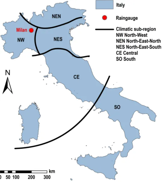
The present scenario (SC0) was defined with regard to a continuous precipitation series observed at the rain gauge of via Monviso (Milan, northwestern Italy). The precipitation was recorded at a 15′ time step for 21 years, between 1971 and 1991. This raingauge belongs to the northwestern climate sub-region NW, according to the analysis byBrunetti et al. (2006b)as shown inFig. 1. Bearing in mind applications to small-medium size urban catchments (10–100 ha), the sampling of the individual independent events from the continuous record was carried out by using an interevent time definition of 3 h and an initial abstraction IA of 5 mm. In these kinds of watersheds, times of concentrations shorter than 1 h are expected, so that the minimum interevent time definition suggested in the literature (Adams and Papa, 2000) can be used to ensure that two subsequent rainfalls do not generate overlapping hydrographs. In addition, owing to the high soil sealing levels, a minimal volume threshold is needed for rainfall to exceed the interception and surface storage losses.

3.1. Present scenario

A summary of statistics of the storm events sampled according to these parameter values is reported inTable 1. Statistics are estimated for the seasonal samples and the whole annual sample, aiming at evidencing the main characteristics of the precipitation regime. InTable 2values of the number of events ˆ, the storm volume µˆhand the wet weather durationµˆdare listed, along with the

Kendall coefficientˆK. The last column reports the total precipitation volume hmaveragely estimated in the various period. These mean values express the rainfall regime traditionally depicted for this climatic region, referred to as sub-alpine regime (Bandini, 1931). The total amount of annual precipitation is about 900 mm, distributed in two wet seasons and two dry seasons. The

main wet season is spring, when most of the events occur, but storm volumes are smaller and wet weather durations are shorter than in the other seasons. Autumn instead represents the secondary rainy season, due to a lower number of events but featured by larger volumes and durations than in spring. Summer and winter differ not only in terms of the total amount of precipitation volumes, since the first is the secondary minimum while the second is the primary minimum, but also in the event number and wet weather durations. In fact, summer features shorter and more frequent storms than winter. In particular, winter wet weather durations are the longest.

This precipitation regime can be explained by considering that during the warm seasons, convective storms are common and short duration events can easily bear large volumes. Conversely, during the cool seasons, such events are almost absent and the

Fig. 1. Italy subdivision according to rainfall trend analysis byBrunetti et al. (2006b)and location of the Milan Monviso raingauge.

Table 2

Sample means µ^ and Kendall coefficients ^Kestimated for the seasonal samples and the whole sample obtained for the Monviso rain gauge series (interevent time definition 3 h, storm volume threshold 5 mm).

Period ^ µ^_h(mm) µ^_d(h) ^_K hm(mm) Winter 7.5 21.1 16.2 0.61 180 Spring 13.4 18.0 8.9 0.42 276 Summer 9.5 20.1 4.7 0.30 209 Autumn 8.9 22.2 12.4 0.43 217 Year 39.3 20.0 10.1 0.37 882

precipitation is mainly driven by frontal events. These characteristics have consequences on the dependence strength, as well. All seasonal samples show concordant associations, though winter events feature a very strong dependence, while summer events feature a quite weak dependence. An intermediate and similar association is instead shown by the wet seasons. Indeed, short duration storms are characterized by a wider variability with respect to long duration storms, as they can be produced by both intense convective events and minor frontal events. The association between storm volumes and wet weather durations is therefore weaker than that of the long duration storms. Hence, smaller Kendall coefficients are thus assessed during the seasons where short duration storms a more frequent.

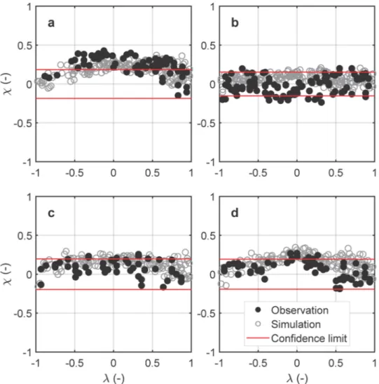
As can be noticed by comparing the seasonal values to the annual ones, the wet weather duration and the association strength appear to be particularly sensitive to seasonality. For instance, summer wet weather durations on average amount to 25 % of the winter ones and to 50 % of the annual ones. Furthermore, the association strength of winter storm variables is double the annual one. The suitability of assessing the pieces of JDF (1) with respect to seasonal samples is therefore clearly supported. In fact, when a storm seasonality of this magnitude is disregarded, FFC derivations basically lead to appreciable underestimations of the peak discharges. The dependence parameters, estimated by using the moment-like criterion based on Eq.(4), are reported inTable 3, along with the results of the statistical tests carried out to evaluate the global goodness-of-fit. As can be seen, the Gumbel-Hougaard copula demonstrates a satisfactory capability to suit the empirical copula in all seasons, due to low Snvalues yielding high p-values. After 105 simulation runs, the null hypotheses cannot be rejected with significances routinely adopted in hydrology, since p-values are larger than 5–10 %, at least. The χ-plots investigating the lower tails and the upper tails in the seasonal samples are plotted inFig. 2and Fig. 3, respectively. In these plots, boundary limits for independence refer to a 10 % test significance. To provide a more effective interpretation of these χ-plots, scatter plots derived from 500 size simulated samples are added to the observed ones in every season. The hypothesis of lower tail independence cannot be rejected in spring (Fig. 2b), in summer (Fig. 2c) and in autumn (Fig. 2d), since observations are close to the λ axis and are included mostly in the confidence boundaries.Fig. 2a instead deserves a deeper discussion, since a significant amount of observations places out of the upper confidence limit. This is mainly due to the high strength of the overall association that generally leads to larger χ values. However, maximum χ values are less than 0.50 and always decrease as λ increases. Moreover, the fitted Gumbel-Hougaard copula appears to be able to satisfactorily mimic the empirical χ-plot, since simulations completely overlap observations. This also applies to the other χ-plots, depicting a general suitability of the tested copula to represent the lower tail behavior.

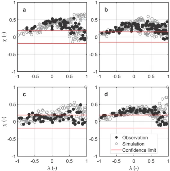
Conversely, the upper tail independence hypotheses can definitively be rejected in winter (Fig. 3a), in spring (Fig. 3b) and in autumn (Fig. 3d), for most of the scatter points are not included in the confidence region testing independence. In the summer case, the overall weak association yields a consistently weak upper tail dependence, so that most of observations remains in the confidence region (Fig. 3c). The χ values exceeding the upper confidence limit nevertheless occur for the largest λ values. This reveals a moderate tendency of the empirical copula to generate associated values in the upper tail. As in the lower tail case, the upper tail dependence appears to be well represented by the Gumbel-Hougaard copula, as simulations fittingly overlap observations in all panels ofFig. 3.

By rejecting the hypotheses of upper tail independence, the comparison of the theoretical value, assessed by Eq.(5), and the empirical values, assessed by estimator (9), of the upper tail coefficients becomes meaningful. Such values are reported inTable 3as well, showing a satisfactory agreement between the theoretical and the empirical coefficients.

Finally, inTable 4and inTable 5the selected marginal distribution functions are listed along with parameter values, estimated by means of the maximum likelihood criterion, and test statistics Dmaxand A2resulting from the Kolmogorov-Smirnov and the Anderson-Darling tests. The corresponding critical limits Dnαand A2refer to a significance α equal to 10 %. As can be seen, all selected distributions cannot be rejected according to both tests, since test statistics are systematically less than the allowed maxima. In general, the Weibull distribution and the gamma distribution are recognized as suitable models for the storm volume and the wet weather duration marginal CDFs, respectively. Exceptions are given by the spring storm volumes and the summer wet weather durations, for which more satisfactory fits were achieved by using the generalized Pareto distribution and the log-normal distribution. In both cases, a little more skewed distribution was needed to better suit the upper tail behavior.

3.2. Climate change scenarios

Changes in the frequency of extremes can be modeled by shifting the overall probability distribution (Simolo et al., 2011), when dealing with threshold exceedance frequency and duration, mainly related to departures from mean values. However, changes in high percentile events, which are of major interest in assessing the hydrologic loads on urban drainage systems, can be represented by changes in the scale parameter and in the shape parameter of the probability distributions (Della-Marta et al., 2007). In this study, to

Table 3

Dependence parameters and test statistics of the Gumbel-Hougaard copulas fitted to the seasonal samples.

Period ^ Sn p-value (%) u ^_u

Winter 2.54 0.018 28.0 0.69 0.65

Spring 1.74 0.022 19.7 0.51 0.49

Summer 1.43 0.012 94.1 0.38 0.38

develop climate change scenarios consistent with seasonal expected trends in northwestern Italy, both methodologies were utilized. Hence, with respect to the present scenario SC0, three change types were implemented in the storm stochastic structure according to the following changes in the seasonal marginal CDFs and in the copula functions:

•

•

•

Changes in storm volumes are supported by forecasts formulated by IPCC future scenarios, in particular, report AR4 (IPCC, 2007) and confirmed by the following studies (IPCC, 2014;Bucchignani et al., 2016). As can be noticed, changes mainly involve a redis-tribution of storm volumes among seasons, maintaining the total amount of annual precipitation virtually constant. Changes in wet weather durations are instead established with regard to a certain number of regional studies concerning trend analyses of daily precipitation series observed in Italy from 1800 to 2003 (Brunetti et al., 2006a;Brunetti et al., 2006c). According to such studies, an average annual decrease of 10 % can be expected in northwestern Italy (seeFig. 1) for the wet weather durations of daily pre-cipitations. Therefore, changes considered in this study must be regarded as moderately conservative, since greater decreases should feature sub-daily storms. This average annual change is modulated with respect to the season, by accounting for moderately greater

Fig. 2. χ-plots testing lower tail dependence properties (10 % significance) for (a) winter storms, (b) spring storms, (c) summer storms and (d)

decreases in those seasons where short duration storms are more frequent, in particular summer. Changes in the marginal dis-tributions can be implemented in JDF (1) independently of those expected for the dependence structure, by modifying the corre-sponding marginal CDFs. A further advantage arises from the utilization of two-parameter marginal CDFs, that makes this im-plementation actually straightforward.

In northern Italy’s climatic region, there are no studies that can address the choice of potential changes in the dependence structure of storm variables. Nevertheless, it is not reasonable to expect a modification of the type of dependence structure, that is of the copula model, but only changes in the dependence strength. This assumption is adopted, for instance, byVinnarasi and Dhanya (2019), who observed a decreasing trend in the dependence parameter of the Frank copula, that relates storm intensities to wet weather durations in Bangalore. In general, the less the dependence strength between the storm volumes and the wet weather durations is, the larger the estimated peak discharges are (Balistrocchi and Bacchi, 2017).

Fig. 3. χ-plots testing upper tail dependence properties (10 % significance) for (a) winter storms, (b) spring storms, (c) summer storms and (d)

autumn storms.

Table 4

Parameters and Kolmogorov-Smirnov (KS) and Anderson-Darling (AD) test statistics of the storm volume CDFs fitted to the seasonal samples (critical values correspond to test significance α = 0.10).

Period Type β ζ(mm) IA (mm) KS AD Dmax Dnα A2 A2 Winter WB 0.88 15.9 5 0.041 0.097 0.350 0.637 Spring GP 0.18 10.85 5 0.043 0.073 0.328 0.596 Summer WB 0.89 14.2 5 0.058 0.086 0.480 0.637 Autumn WB 0.88 16.3 5 0.041 0.089 0.462 0.637

Aiming at evidencing the advantages of the proposed stochastic methodology and by evaluating the impact of changes in the storm structure on flood frequency, a reasonable scenario can however be derived by the assessment of trends in the Monviso rainfall series. By using a mobile window equal to five years, a slight decreasing trend in the Kendall coefficient is evidenced for the annual samples. Nevertheless, when annual samples are separated into seasonal samples, only summer storms show such a behavior. Winter storms and autumn storms instead show more marked decreasing trends, the first being the strongest one, while spring storms show a moderate increase. Such results addressed the previously outlined changes in the dependence strength.

Climate change scenarios are therefore developed as follows: scenario 1 (SC1) accounts only for trends in the storm volume CDFs, scenario 2 (SC2) accounts for both trends in the marginal CDFs and scenario 3 (SC3) accounts for trends in the marginal CDFs and in the dependence structure. Scenario 1 is intended to evaluate the FFC trend in the sub-regions of northern Italy where wet weather duration trends are not expected. Distinguishing between scenario 2 and scenario 3 makes it possible to quantify the effect of disregarding changes in the storm variable dependence structure on flood frequency.

4. Results and discussion

The proposed stochastic methodology was initially tested by model comparison. This is a broadly used approach to validate derived models that are applied to urban drainage systems (Guo and Adams, 1998,1999;Balistrocchi et al., 2009;Zhang and Guo, 2014,2015;Wang and Guo, 2019), due to the general scarcity of long-term series of observed discharges. A benchmarking reference was set up through continuous simulations of a hydrodynamic model developed in SWMM (Environmental Protection Agency, 2015), with regard to a hypothetical, but realistic, test case. The stochastic methodology was then applied to various watershed outlets, according to the climate change scenarios delineated in section3.2.

Table 5

Parameters and Kolmogorov-Smirnov (KS) and Anderson-Darling (AD) test statistics of the wet weather duration CDFs fitted to the seasonal samples (critical values correspond to test significance α = 0.10).

Period Type β ζ(h) KS AD Dmax Dnα A2 A2 Winter GM 2.77 5.85 0.056 0.097 0.571 0.639 Spring GM 1.48 5.98 0.041 0.073 0.411 0.643 Autumn GM 1.96 6.33 0.053 0.089 0.578 0.643 Period Type μln h σln h KS AD Dmax Dnα A2 A2 Summer LN 1.12 0.92 0.060 0.086 0.476 0.631

4.1. Stochastic model verification

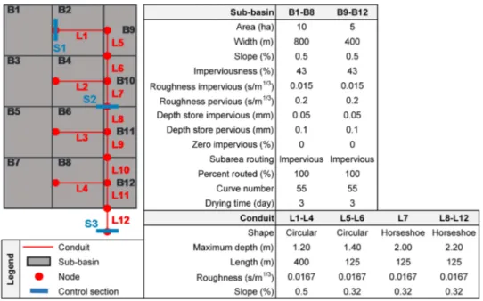
The test watershed delineates a recurrent runoff management strategy adopted in urban drainage systems. As can be seen in Fig. 4, where the topologic scheme of the drainage network is illustrated, secondary parallel pipes connect to a main interception conduit. This conduit features a larger cross section and a lower slope than secondary pipes. The total catchment area amounts to 100 ha and is subdivided in ten sub-basins. Major sub-basins drain into the secondary pipes and are approximated to rectangular plains, symmetrically sloping towards to a central gutter flow path. Minor sub-basins directly drain into the interception conduit and are approximated to rectangular plains completely located on the left-hand side of the gutter flow path. Overland flow widths are therefore estimated as twice and equal to the gutter path length, for major sub-basins and minor sub-basins respectively. The drologic losses that occurr in the permeable areas were estimated by using the curve number method. Details regarding the hy-drologic and hydraulic characteristics of sub-basins and pipes implemented in the SWMM hydrodynamic model are provided in Fig. 4, as well.

The parameterization of the stochastic model was carried out aiming at maximizing the consistency with hydrodynamic simu-lations. In particular, the runoff coefficient Φ defined in Eq.(10)was set with regard to the discretization procedure described in section2.1. Hence, the rainfall excess series was obtained from the rainfall series by subtracting the hydrologic losses from the independent storm events separated by an interevent time definition of 3 h. The runoff coefficient was set in order to obtain, for the complete observation period, a ratio between the runoff volume and the rainfall volume equal to that resulting from SWMM con-tinuous simulations. Since it is applied only to the rainfall portion exceeding the initial abstraction, this runoff coefficient is basically larger than those usually adopted in urban drainage systems, which apply to the total rainfall volume.

The watershed time of concentration tcwas estimated by using Eq.(14)as the sum of the time needed for the runoff to enter the drainage network teand the time needed for the channelized runoff to reach the outlet section through the longest hydraulic path. The second addend is computed as the sum of the delivery times of the single pipes, estimated as the ratio between pipe length ljand flow velocity vj = + t t l v c e j j j ₍₁₄₎

With the aim of highlighting a potential influence of the watershed size on the agreement between the hydrodynamic model and the stochastic model, FFCs were derived for three control sections depicted inFig. 4, corresponding to catchment areas equal to 10 ha (section S1), 50 ha (section S2) and 100 ha (section S3). Corresponding calibration parameters are listed inTable 6. Times of concentrations were set by adopting 10 min for teand 1.5 m/s for velocities vj. In particular, the first is suggested in northern Italy climate for urban watershed practical applications (Centro Studi Idraulica Urbana (CSDU, 1997), whereas the latter is intended to represent runoff delivery velocities related to the most frequent storms, that features low-moderate intensities. A runoff coefficient Φ equal to 0.75 coupled with an initial abstraction IA equal to 5 mm yields a ratio between the total runoff volume and the total rainfall volume of 50.3 %, that is consistent with that obtained through the hydrodynamic simulation assessed at 50.5 %.

Monte Carlo simulations were conducted by generating 2.5 104_{years of storm volume and wet weather duration couples in} accordance with the parameter set reported fromTable 2toTable 5(SC0). Such couples were transformed in peak discharges by using Eq.(12)and associated with the corresponding return period by using Eq.(13). The continuous flow discharge series simulated in the three analyzed sections by SWMM were separated into independent runoff events by using a threshold discharge and an interevent time definition equal to 3 h. The threshold discharges were set at a few hundreds of liters per second, to purge out of the series the insignificant low flow. The interevent time definition is consistent with that used in the rainfall series analysis.

The visual comparison of the FFCs is provided inFig. 5and performance measures of the stochastic model are listed inTable 6. As can be seen inFig. 5, FFCs derived by the proposed stochastic model (MC) and by continuous hydrodynamic simulations (SWMM) depict similar trends. Assessments are particularly close for the peak discharges featuring return periods greater than 2 years, which are of major interest for practical application purposes. The satisfactory agreement is also evidenced by the root mean square errors (RMSE), reported inTable 6, which can be considered acceptable with respect to the order of magnitude of the peak discharges. The Nash-Sutcliffe efficiency (NSE), that is a normalized version of the mean square error, further confirms this performance evaluation due to values always larger than 0.80. An additional quantitative evaluation of the stochastic model performances is provided by the Pearson linear correlation coefficient (LCC), whose values are satisfactorily near to unity.

Table 6

Calibration parameters and performance evaluation measures of the stochastic model: root mean square error (RMSE), Pearson linear correlation coefficient (LCC) and Nash-Sutcliffe efficiency (NSE), obtained by assuming hydrodynamic simulations as a benchmark.

Section Area (ha) IA(mm) Φ t(h)c RMSE (m 3_{/s) LCC NSE} 1 10 5 0.75 0.26 0.089 0.98 0.83 2 50 5 0.75 0.40 0.389 0.97 0.85 3 100 5 0.75 0.49 0.543 0.99 0.91

Fig. 5. Comparison of FFCs derived from the rainfall series observed at Monviso raingauge in three different sections of the test watershed, by using

the proposed stochastic model and the SWMM hydrodynamic model.

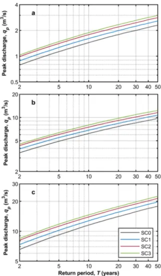
Fig. 6. Flood frequency curves derived according to the analyzed scenarios for the three sections of the test watershed: (a) S1 10 ha, (b) S2 50 ha e

4.2. Stochastic model application

InFig. 6, FFCs derived by means of the stochastic procedure in accordance with the described scenarios of climate change are compared to those derived in accordance with the present climate SC0. Such examples refer to the three sections of the test watershed (Table 6), used in section4.2to verify the soundness of the stochastic model. As can be seen, all climate change scenarios determine significant increases in the flood frequency, whose percentage values appear to be almost constant with respect to both the return period and the catchment area. With regard to the return period range of major interest for urban practical applications (2–20 years), SC1 yields percentage increases of about 10–12 % with respect to SC0 FFCs.

Moreover, when SC1 and SC2 are compared additional percentage increases in the flood frequency ranging between 10–12 % arise, thus the total percentage increases reach 20–24 % with respect to SC0. More limited increments are instead predicted if changes in the volume-duration dependence structure are considered. If FFCs derived for SC2 and SC3 are compared, additional percentage increases range between 5–6 %, so that the total percentage increase with respect to SC0 is estimated at 28–29 %. This result can be explained by considering that FFCs in urban watersheds are mainly determined by short duration storms. In this climate, such storms mainly occur in summer and subordinately in spring and autumn. A very moderate change was adopted for summer and opposite change trends were implemented for spring storms and autumn storms in the Monte Carlo generation procedure.

Such results however demonstrate that moderate changes in the temporal structure of storms have dramatic impacts on flood frequency in urban watersheds, and that the expected increases in the peak discharges are, at least, of the same magnitude as those due to changes in the storm volume seasonality. In order to demonstrate the significance of the predicted increases regarding the runoff management in urban watersheds, a term of comparison is provided by the conveyance capacities of conventional drainage systems. To do so, one can refer to the ratio between the peak discharge and the full normal flow discharge, which expresses the pipe conveyance capacity. This ratio is routinely included in the safety range spanning from 0.70 to 0.80, in order the conveyance capacity to be considered suitably sized. Assuming that a drainage pipe is included in the safety range under the present scenario SC0, the ratio increases up to 0.78–0.90, according to SC1, up to 0.85–0.98 according to SC2, and up to 0.90–1.03 according to SC3. These ranges therefore predict situations in which drainage pipes are undersized or heavily undersized, with respect to the original design return period.

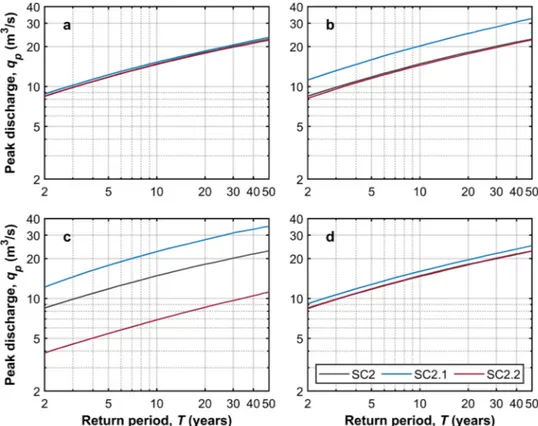
To better investigate the impact of potential changes in the dependence structure of storm variables on flood frequency, a sensitivity analysis was conducted by individually changing the seasonal Kendall coefficients within the maximum possible range. Hence, the independence (τk= 0) and the analytical concordant association (τk= 1) were implemented into the stochastic derivation procedure, by substituting the Gumbel-Hougaard copula with the product copula (Π2copula) and the upper boundary copula (M2 copula), respectively. Results are illustrated inFig. 7, where FFCs derived according to these assumptions are compared to the those

Fig. 7. Sensitivity analysis of FFCs with respect to seasonal dependence strength of storm volumes and wet weather durations: independence SC2.1

derived by keeping the dependence structure stationary (SC2).

In all cases the decrease in the association strength leads to an increase in the flood frequency, while the contrary occurs when the association is increased. Nevertheless, impacts on FFCs are highly different with regard to the season. The most relevant impact is evidenced in summer (Fig. 7c), when the largest variation can be observed. In particular, the independence assumption leads to an increase of 56.5 % and the analytical concordant association leads to a decrease of 50.0 % in the peak discharges. This outcome can be explained by considering that the majority of short duration and intense storms occur in this season. Such a kind of storm is the most critical for the watersheds herein analyzed, which are characterized by times of concentration less than an hour. Conversely, the impact of dependence strength changes in winter appears to be definitively negligible (Fig. 7a). This season is actually rich in stratiform storms, which are not able to significantly force the urban drainage system, due to their basically long durations coupled with low intensities.

Intermediate results are shown in spring (Fig. 7b) and in autumn (Fig. 7d), which feature a mixture of stratiform storms and convective storms. In both seasons the most relevant impact is due to the independence assumption, which would yield a marked increase in the peak discharges of 40.0 % when spring is considered. A modest increase of about 12.5 % is instead predicted by neglecting the association strength in autumn. The almost null effect of the association strength increase can be explained by the modest impact that the storms belonging to these seasons have on the FFCs and by the moderately high concordance that already characterizes the observed samples. In general, it must be concluded that individual seasonal trends in the storm volume and wet weather durations can have dramatic consequences on the flood frequency, when the season featuring the majority of the storms critical to the analyzed drainage system is taken into consideration.

5. Conclusions

In this paper, a stochastic methodology to derive flood frequency distributions from precipitation inputs in small-medium sized urban watersheds (that is featuring catchment areas between 10 ha and 100 ha) was proposed. A bivariate approach incorporating the seasonality of storm volumes and wet weather durations was implemented in a computationally cheap simulation procedure (section2). This procedure was applied and tested with reference to an urban watershed located in northwestern Italy. In this climate a 21-year long series of precipitation volumes recorded every 15′ is available (Milan Monviso raingauge).

Copula functions were exploited to carry out a comprehensive seasonal investigation of the precipitation temporal structure (section3.1). In this regard, the distribution of convective storms is acknowledged as a fundamental factor affecting both the overall dependence strength and the scale parameters of the marginal variables. Copulas were used to construct joint distribution functions satisfactorily suiting the empirical distributions of the storm event variables. In particular, members of the Gumbel-Hougaard family were found to provide suitable representations of the global dependence structures (Table 3), the lower tail dependences (Fig. 2) and the upper tail dependences (Fig. 3) in all seasons.

The overall model reliability was verified with respect to hydrologic-hydraulic continuous simulations conducted by using EPA SWMM (Fig. 5). Even if a simplified precipitation runoff transformation model was implemented in the stochastic derivation pro-cedure, its flood frequency curves demonstrated to be in close agreement with those derived by a hydrologic-hydraulic model, at spatial scales ranging from 10 ha and 100 ha. Considering the magnitude of the peak discharges related to the tested urban wa-tershed, estimate errors are found to be acceptable.

Potential impacts of climate change on the flood frequency distributions were estimated by accounting for trends of storm volumes, wet weather durations and their mutual dependence strength. In doing this, the probabilistic representation of the pre-cipitation process provided by the copula functions made it possible to implement such trends in the derivation procedure in a very straightforward and computationally efficient manner (section3.2). Taking into account changes in the temporal structure of storms leads to significant variations in the derived distribution of flood frequency. In particular, appreciable changes are expected in the flood frequency even when only the dependence strength of the storm variables is changed (Fig. 6). Such aspects therefore deserve to be carefully investigated when facing the assessment of the impact of precipitation non-stationarity on the runoff processes. A special focus must be given to the season featuring the majority of storms that are critical for the analyzed drainage systems. In the ap-plication presented in this study, this season is summer (Fig. 7), when convective storms with short durations and high intensities are common.

The proposed approach appears to be more convenient with respect to the hydrologic-hydraulic continuous simulations, since changes in the mean values or in the high percentile values of the climate variable can be represented by simply modifying the scale and the shape parameters of the marginal distributions. Further advantages arise from the possibility to avoid computationally intensive numerical simulations and to extrapolate the flood frequency assessment to return periods larger than the length of the available precipitation series. Moreover, it is worth noting that changes in the dependence structure of storm variables are hardy implementable in conventional hydrodynamic simulations, since they can be accounted for by generating a sufficiently large number of precipitation time series, to be used as an input for the hydrodynamic models. Thus, a prohibitive computational burden should be dealt with.

Finally, specific results can be drawn for urban watersheds located in the analyzed climate of northwestern Italy (Fig. 6). The assessed impacts demonstrated to be significant in the control of urban runoff by means of conventional drainage systems, even though the total annual precipitation volume is expected to remain virtually constant. As a consequence of the combination of the storm volume regime redistribution, the wet weather duration shortening and a moderate decrease in the dependence strength, drainage systems are expected to fail more frequently yielding more severe flooding episodes. Actually, with respect to the return period conventionally adopted in Italy for the drainage network design, the estimated increases in the hydrologic loads largely exceed

the safety range of the conveyance capacity.

Future research developments regarding the proposed stochastic model are manifold. On the one hand, they could be addressed to additional applications, such as the design and performance assessment under non-stationary conditions of drainage pipes, combined sewer overflow devices, runoff capture tanks or flood control reservoirs. They could also include quality control issues, by adding further steps in the derivation procedure to represent the transport phenomena of non-point contaminants. On the other hand, in consideration of the impact that the temporal structure of storms can exert on the flood frequency, extensive and comprehensive studies on trends in wet weather durations and their statistical relationship with storm volumes should be undertaken to recognize potential threats to urban drainage systems. Bearing in mind the short times of concentration characterizing such watersheds, heavy storms are associated with short wet weather durations, therefore event-based analyses on sub-hourly precipitation records must be systematically investigated.

Acknowledgement

This paper received funding from the European Union’s Horizon 2020 Research and Innovation Programme under grant 741657, with the name SciShops.eu. The content of this article does not reflect the official opinion of the European Union. Responsibility for the information and views expressed in the article lies entirely with the authors.

References

Abberger, K., 2005. A simple graphical method to explore tail-dependence in stock-return pairs. Appl. Financ. Econ. Lett. 15 (1), 43–51.

Adams, B.J., Howard, C.D.D., 1986. Design storm pathology. Can. Water Resour. J. 11 (3), 49–55.

Adams, B.J., Papa, F., 2000. Urban Stormwater Management Planning with Analytical Probabilistic Models. John Wiley & Sons, New York.

Akan, A.O., Houghtalen, R.J., 2003. Urban Hydrology, Hydraulics and Stormwater Quality. John Wiley & Sons, Hoboken, NJ.

Alexander, L.V., et al., 2006. Global observed changes in daily climate extremes of temperature and precipitation. J. Geophys. Res. Atmos. 111 (5), D05109.

Arnbjerg-Nielsen, K., Willems, P., Olsson, J., Beecham, S., Pathirana, A., Bülow Gregersen, I., Madsen, H., Nguyen, V., 2013. Impacts of climate change on rainfall extremes and urban drainage systems: a review. Water Sci. Technol. 68 (1), 16–28.

Bacchi, B., Balistrocchi, M., Grossi, G., 2008. Proposal of a semi-probabilistic approach for storage facility design. Urban Water J. 5 (3), 195–208.

Balistrocchi, M., Bacchi, B., 2011. Modelling the statistical dependence of rainfall event variables through copula functions. Hydrol. Earth Syst. Sci. Discuss. 15 (3), 1959–1977.

Balistrocchi, M., Bacchi, B., 2017. Derivation of flood frequency curves through a bivariate rainfall distribution based on copula functions: application to an urban catchment in northern Italy’s climate. Hydrol. Res. 48 (3), 749–762.

Balistrocchi, M., Bacchi, B., Grossi, G., 2009. An analytical probabilistic model of the quality efficiency of a sewer tank. Water Resour. Res. 45 (12), W12420.

Balistrocchi, M., Grossi, G., Bacchi, B., 2013. Deriving a practical analytical-probabilistic method to size flood routing reservoirs. Adv. Water Resour. 62, 37–46.

Bandini, A., 1931. Tipi Pluviometrici Dominanti Sulle Regioni Italiane. Servizio Idrografico Italiano, Roma, IT in Italian.

Barone, L., Pilotti, M., Valerio, G., Balistrocchi, M., Milanesi, L., Chapra, S.C., Nizzoli, D., 2019. Analysis of the residual nutrient load from a combined sewer system in a watershed of a deep Italian lake. J. Hydrol. (Amst) 571, 202–213.

Becciu, G., Raimondi, A., 2012. Factors affecting the pre-filling probability of water storage tanks. WIT Transactions on Ecology and the Environment 164, 473–484.

Brunetti, M., Maugeri, M., Monti, F., Nanni, T., 2006a. Temperature and precipitation variability in Italy in the last two centuries from homogenised instrumental time series. Int. J. Climatol. 26 (3), 345–381.

Brunetti, M., Maugeri, M., Nanni, T., 2006b. Trends of the daily intensity of precipitation in Italy and teleconnections. Il Nuovo Cimento Ser. 5 29 (1), 105–116.

Brunetti, M., Maugeri, M., Nanni, T., Auer, I., Böhm, R., Schöner, W., 2006c. Precipitation variability and changes in the greater alpine region over the 1800-2003 period. J. Geophys. Res. Atmos. 111 (11), D11107.

Bucchignani, E., Montesarchio, M., Zollo, A.L., Mercogliano, P., 2016. High-resolution climate simulations with COSMO-CLM over Italy: performance evaluation and climate projections for the 21st century. Int. J. Climatol. 36 (2), 735–756.

Centro Studi Idraulica Urbana (CSDU), 1997. Sistemi Di Fognatura Manual Di Progettazione. EdiBios, Castrovillari (IT) in Italian.

Della-Marta, P.M., Haylock, M.R., Luterbacher, J., Wanner, H., 2007. Doubled length of western European summer heat waves since 1880. J. Geophys. Res. Atmos. 112, D15103.

Donat, M.G., et al., 2013a. Updated analyses of temperature and precipitation extreme indices since the beginning of the twentieth century: the HadEX2 dataset. J. Geophys. Res. Atmos. 118 (5), 2098–2118.

Donat, M.G., Alexander, L.V., Yang, H., Durre, I., Vose, R., Caesar, J., 2013b. Global land-based datasets for monitoring climatic extremes. Bull. Am. Meteor. Soc. 94 (7), 997–1006.

Dong, X., Guo, H., Zeng, S., 2017. Enhancing future resilience in urban drainage system: green versus grey infrastructure. Water Res. 124, 280–289.

Dotto, C.B., Mannina, G., Kleidorfer, M., Vezzaro, L., Henrichs, M., McCarthy, D.T., Freni, G., Rauch, W., Deletic, A., 2012. Comparison of different uncertainty techniques in urban stormwater quantity and quality modelling. Water Res. 46 (8), 2545–2558.

Dupuis, D.J., 2007. Using copulas in hydrology: benefits, cautions, and issues. J. Hydrol. Eng. 12 (4), 381–393.

Eagleson, S.P., 1972. Dynamic of flood frequency. Water Resour. Res. 8 (9), 878–898.

Elliott, A.H., Trowsdale, S.A., 2007. A review of models for low impact urban stormwater drainage. Environ. Model. Softw. 22 (3), 394–405.

Environmental Protection Agency, 2015. In: Rossman, L.A. (Ed.), Storm Water Management Model User’s Manual Version 5.1. US Environmental Protection Agency. EPA 600/R-14/413b.

Favre, A.-C., El Adlouni, S., Perreault, L., Thiémonge, N., Bobée, B., 2004. Multivariate hydrological frequency analysis using copulas. Water Resour. Res. 40, W01101.

Fisher, N.I., Switzer, P., 1985. Chi-plots for assessing dependence. Biometrika 72 (2), 253–265.

Fisher, N.I., Switzer, P., 2001. Graphical assessment of dependence: is a picture worth 100 tests? Am. Stat. 55 (3), 233–239.

Frahm, G., Junker, M., Schmidt, R., 2005. Estimating the tail-dependence coefficient: properties and pitfalls. Insur. Math. Econ. 37 (1), 80–100.

Fu, G., Kapelan, Z., 2013. Flood analysis of urban drainage systems: probabilistic dependence structure of rainfall characteristics and fuzzy model parameters. J. Hydroinf. 15 (3), 687–699.

Genest, C., Favre, A.-C., 2007. Everything you always wanted to know about copula modeling but were afraid to ask. J. Hydrol. Eng. 12 (4), 347–368.

Genest, C., Rémilland, B., Beaudoin, D., 2009. Goodness-of-fit tests for copulas: a review and a power study. Insur. Math. Econ. 44 (2), 199–213.

Grimaldi, S., Serinaldi, F., 2006. Asymmetric copula in multivariate flood frequency analysis. Adv. Water Resour. 29 (8), 1115–1167.

Guo, Y., Adams, B.J., 1998. Hydrologic analysis of urban catchments with event-based probabilistic models. 2. Peak discharge rate. Water Resour. Res. 34 (12), 3433–3443.

Guo, Y., Adams, B.J., 1999. An analytical probabilistic approach to sizing flood control detention facilities. Water Resour. Res. 35 (8), 2457–2468.

Hartmann, D.L., et al., 2013. Observations: atmosphere and surface. In: Stocker, T.F. (Ed.), Climate Change 2013: The Physical Science Basis. Cambridge University Press, UK, pp. 159–254.