Noise and vibration characteristics of a micro car diesel engine

A dissertation presented

to the Faculty of Engineering of

The University of Roma Tre

by

Sunny Narayan

in Partial Fulfillment of Requirements

for the Degree of

Doctor of Philosophy

The University of Roma Tre

May 2016

Dedication

and support of so many people. I am thankful to all who have supported me during course of my study of Phd study period at ′ The University of Roma Tre′. First and foremost, of all I would like to thank my advisors Prof. G. Chiatti and Prof. O. Chiavola who gave me this wonderful opportunity to study in their research group. Without their support and guidance, none of this work would have been possible. During my period of study, they supported and advised me by reviewing my work continuously. These years of study at ′ The University of Roma Tre′, have helped me to gain the requisite knowledge.

I am also grateful to Ing. F. Palmieri, PhD and Mr. Rashid Ali, PhD for their initial support and guidance. I would also like to express my gratitude to Ing. Erasmo Recco for his support to carry out various experimental activities and who spent hours to help me out in this work.

I thank all my family members who were constant source of support and inspiration for me. My sincere thanks goes to people in DOMUS SRL group including Mrs. Ellena and Mr. Trulli Carlo who were always there to provide me any logistic support.

It was a challenging period of my life and I have enjoyed it gaining the expertise to grow as a professional. Rome, 3rd April 2016.

Sunny Narayan

Declaration

I, Sunny Narayan do hereby declare that this thesis titled '' Noise and vibration characteristics of a micro car diesel engine '' and the work involving it are results of my own research. I further confirm that:

a) The work has been done while in candidature for a research degree at this University.

b) No part of this work has been previously submitted for award of any degree /qualification at this University or any other university or institution.

c) Wherever I have quoted from the work of others, the source has been always given. d) I have acknowledged all major sources of help.

e) Wherever the portions of work presented in this thesis was done by myself jointly with others, I have made clear exactly what was done by others and what I have contributed myself.

Signature: Date :03/04/2016

parameters that provide information about its working conditions. Due to several drawbacks of various conventional techniques used, novel methods of condition monitoring are becoming the next hot topic of research for major automotive companies around the world.

Diesel engines have been widely used for a variety of industrial as well as domestic applications. Despite their advantages in terms of fuel economy (as compared to gasoline engines), these engines are often less popular due to their worst performance in terms of noise, vibration and harness (NVH) benchmarks. Hence it is important to develop a suitable scheme which is capable enough to detect faults by monitoring various signals acquired from these engines before actual breakdown takes place.

In this work, data was collected from a dual cylinder diesel engine installed in the laboratory of Internal combustion engine at ʹUniversity of Roma Treʹ by changing speed, load, amount and duration of fuel injected. The collected data was further processed using various MATLAB based processing tools. The presented work also discusses various numerical models based on mathematical analysis. The discussed research work has following major objectives:

Objective 1-To review different sources of noise in engines.

Objective 2-To study the effects of variations of different engine operational conditions on various signals acquired from transducers mounted on the test engine.

Objective 3- To show the applicability of various signal processing methods for effecting condition monitoring of engines.

Objective 4-To analyze combustion based noise using acquired data.

Objective 5-To develop various numerical models of piston lateral motion and validate them using experimental data.

Objective 6-On the background of presented work, provide a guideline for further research.

The presented work has been organized into six chapters. Basic principles of noise, vibration and harness (NVH) have been presented in the first two chapters. Chapter 1, analysis different sources of noise in an engine and briefly discusses various techniques used for effective separation of these sources. Chapter 2 discusses various signal processing methods adopted for diagnosis of different signals acquired. Chapter 3 focuses on various characteristic features of various sources of noise in an engine. Chapter 4 deals with combustion based noise and discusses use of in cylinder pressure, noise emissions and engine block vibration signals for its analysis. Chapter 5 is deals with noise emissions due to lateral motion of piston assembly. The dynamic equations of lateral motion of skirt were solved and effects of various parameters were analyzed. Chapter 6 presents a summary of various results and relates it to previous objectives presented. Further suggestions have also been made for future research work.

The novelty of methods discussed in the presented work lies in analysis of various combustion noise related indices which showed a good correlation with actual in cylinder pressure development. Further various mathematical models have been used for analysis of lateral motion of skirt and effects of various skirt design parameters on it.

As the output signals from various transducers mounted on the test engine are available at an early stage, various methods discussed in the presented work may become an attractive option for effective detection and localization of various faults and hence, form an important aspect of preventive maintenance of engines.

Keywords: Diesel engines, in cylinder pressure, noise, vibrations and harness. VI

Table of Contents

List of Symbols

List of Figures

List of Tables

Chapter 1

Introduction

1.2 Summary of various sources of noise in combustion engines………....………...….2

1.3 Quantification of noise emissions from engines………..………...…4

1.4 Methods for quantification of noise emissions………...……….………...………...….6

1.5 Summary………..….10

1.6 References………...10

Chapter 2

Methodology for condition monitoring in engines

2.2 Signal processing tools……….………...…….….……...…...14

2.3 Experiments………..………...………..……..15

2.4 Results and discussions……….………..……….…....15

2.5 Summary ………...……...………...…24

2.6 References………...………...……….……….…...24

Chapter 3

Features of various sources of noise in engines

3.2 Combustion noise………27

3.3 Piston assembly noise……….………...…...27

3.4 Valve train noise……….……….…..…..28

3.5 Gear train noise………...………...….28

3.6 Crank train and engine Block vibrations……….………...29

3.7 Aerodynamic noise………..………29

3.8 Bearing noise………...………...29

3.9 Timing belt and chain noise………...…..………...29

3.10 Summary……….…………..………31

3.11 References ………....………...…….…32

4.1 Introduction………..……….34

4.2 Background of Combustion Process in Diesel Engines………..………....….….34

4.3 Combustion Phase analysis……….……….…....….36

4.4 Combustion Based engine noise ……….………..……..….49

4.5 Factors effecting combustion noise……….…..56

4.6 Effects of heat release rate ……….………..………...57

4.7 Effects of cyclic variations………....………...…….57

4.8 Resonance phenomenon………...………...….58

4.9 In cylinder pressure decomposition method……….………….…...….58

4.10 Mathematical Model of Generation of Combustion Noise………...…………..……..59

4.11 Methods to evaluate combustion noise ………..…………..…...…63

4.12Summary………...…….………65

4.13 References………...……..66

Chapter 5

Piston Slapping Noise

5.2 Background………...71

5.3 Reynolds equation for lubrication oil pressure distribution ……….…72

5.4 Occurrence of Piston Slap Events………...77

5.5 Piston Motion analysis using software………....…………..…….81

5.6 Force Analysis………...83

5.7 Effects of various skirt design parameters on lateral motion of skirt………....…86

5.8 Numerical model of slapping motion………..………..92

5.9 Driving forces………....…………..………..92

5.10 Determination of mobility ………..………..…..93

5.11 Results and discussions………...……..………95

5.12 Summary………...………..………...97

5.13 References ……….………..……...97

Chapter 6

Conclusions and future work

6.2 Resume state of art………..……….………...100

6.3 Overall Conclusions………...………...102 6.4 Innovation Introduced………...………...…………...………...103 References………...……...………...103

List of publications

Appendix

List of Symbols

a- Dilation parameter b- Translation parameter

Ar -Area of noise radiating surface

Ac- Proportionality coefficients A-Cylinder surface area

A.T.S.-Anti thrust side ATDC-After top dead center

ap - Location of connecting rod from its top part of skirt

B-Cylinder bore b (f)-Radiation rate

bc -Distance of skirt center of mass from its top part

BEM-boundary element method

BTDC-Before top dead center C-Speed of sound

C(t)-Output response

CV(h)-The covariance of a given function x(h)

C~_{(t)-Approximation of combustion noise}

CWT (a, b)-Complex wavelet transform

Cp,a (f)-Coherence function between in-cylinder pressure block vibration signals

CHRR- Cumulative heat release rate C-Speed of sound

C(f)- Decay constant

Cθ- Torsion damping coefficient of skirt

Cc-Wave propagation speed

Cb-Dynamic damping coefficient of engine block

Cp-Dynamic damping coefficient of skirt

CI, Ƶ -Combustion Index Cp, dp-Pin offset distance

CN-Combustion noise levels C-Crank case offset

ca -Wave speed

dBA- A weighted sound pressure level dB -Decibel level

D-Number of teeth D-Piston diameter D.I.-Direct injection

dCOG , Cg-Center of gravity offset

EVO-Exhaust valve opening EVC-Exhaust valve closure EA-Impact energy

ECN-End of combustion noise E(t)-Total noise emissions

E(f)- Available energy at engine surface et –Top eccentricity

eb -Bottom eccentricity

F(f) -Force applied at top of piston fs -Excitation frequency

f(ω)-Fourier transformation of a function f(t) f – Frequency

fg –Gas resonance frequency

fr -Resonant frequency

fc - Central frequency

fb - Bandwidth

fmean-The mean frequency of a signal

Ft ,Fx- Lateral force on liner

Ff - Frictional force between liner and skirt

Ffr- Frictional force between liner and rings

FFT-Fast Fourier transformations FEA-Finite element analysis

FIC -Inertial force acting along X axis

F⎺IC -Inertial forces along Y axis

F~

I,J - average of local force

G~_{(t)- Approximation of mechanical noise}

Gx(f)-Input function spectrum

Gy(f)- Output function spectrum

Gh(f)-Transfer function spectrum

H1- Transfer function of combustion noise

h-Oil film thickness h(t-τ) - Window function

h͞ - Dimension less oil film thickness H(t)- Impulse response

HCCI-Homogenous charge compression ignition IVC-Inletvalve closure

IVO-Inlet valve opening IO -Overall intensity of noise

I(f) -The intensity of radiated noise I- Intensity of combustion noise

IFFT-Inverse Fast Fourier transformations J, I piston -Piston skirt having moment of inertia

Kb-Dynamic stiffness of engine block

K p-Dynamic stiffness of skirt

K θ-Torsion stiffness coefficient of skirt

L w[A]-A weighted sound power level of engine

L-Axial length

Lx-Horizontal offset of center of gravity from pin position

Ly-Vertical offset of center of gravity from pin position

L-Skirt length

l – Connecting rod length

LPP-Location of peak pressure rate

LMA -Least value of filtered accelerometer signals

MA -Modal analysis

M z-Total Moment about the wrist-pin

Mf -Moment of Ff about the wrist-pin

MIC -Rotatory moment about wrist pin

mb-Dynamic Mass of engine block

Mb-Dynamic mass of engine block

m piston -Skirt mass

m sl-Small end connecting rod mass

m t -Total mass of pin, skirt and small end of connecting rod

M h -Moment of oil force about piston pin

m piston -Mass of skirt

m pin -Piston pin mass

MN-Mechanical noise levels

MBF50 - Crank angles locations at which 50% of fuel is burnt MBF100-Crank angles locations at which 100% of fuel is burnt MPRR-Peak pressure rise rate

M(t)- Corrupted component/Mechanical noise M p-Dynamic mass of skirt

M z-Moment about piston pin

NI-Noise Index N -Engine RPM

N ideal -Ideal engine speed

NVH- Noise, vibration and harness ON-Overall noise levels

(dP

𝑑𝑡)𝑝𝑖𝑙𝑜𝑡 - Maximum pressure gradient during pilot injection period (dP

𝑑𝑡)𝑚𝑎𝑖𝑛 -Maximum pressure gradient during main injection ((dP

𝑑𝑡)𝑚𝑜𝑡𝑜𝑟𝑒𝑑 -Maximum pressure gradient in motored pressure signal P injection -Injection pressure

P max -Maximum pressure value

P residual-Residual pressure levels

P Motored -Motored pressure levels

PCCI-Pre-mixed charge compression ignition p(x, θ) −Non linear oil pressure distribution Pa -Acoustic power available at surface

P-Oil pressure distribution

P(fk)- kth sample of power spectrum and w is signal frequency band

p(f)-Pressure spectrum p-In cylinder pressure PH-Pitch

Pp, a -Cross PSD function between in-cylinder pressure block vibration signals

Pp, P -Auto PSD function of in-cylinder pressure

Pa, a -Auto PSD function of block vibration signals

Pv- Impact power

Pv- Impact force

(dP

𝑑𝑡)𝑚𝑎𝑥 -Maximum rate of pressure rise P(t) –Input response

p͞ - Dimension less oil pressure (dP

𝑑𝜃) -Rate of pressure rise (PRR) (dQ

𝑑𝜃) -Rate of heat release (ROHR) Q- Amount of heat released(J)

Q pre -Amount of fuel injected in pre-injection period

Q pre -Amount of fuel injected main-injection period

qm, n -Modes of resonance frequency

r, rp-Crank radius

S-Radiated surface area S-Stroke length

SEA-statistical energy analysis

SCN- Start of combustion noise SPL-Sound pressure levels SPP(f) - Auto spectrum of P(t)

SPD(f) -Cross spectrum of P(t) and E(t)

SOI pre-Start of pre-injection period

SOI main- Start of main-injection period

STFT (τ, f)-The short time frequency analysis t͞ - Dimension less time

Tp-Rotation torque about piston pin

Tf -Frictional torque

TG -Gas torque

TDC-Top dead center T.S.-Thrust Side

TPA- Transfer path analysis

u- Surface velocity

V - In cylinder volume V-Skirt velocity along Y axis vr -Surface velocity

Vv -Impact velocity

WI,J-Energy transferred to each grid point

W- Velocity along Z axis Wc -Combustion impact power Wn -Combustion noise power W(t)-Spectro filter response WA -Impact speed of roller

W-Radiated acoustic power X m-Discrete function

x(t) - Input signal

x^(h)-Hilbert transformation of function x(h) x+' _{-Complex conjugate of x}+

x͞ -Dimension less X coordinate 𝑋𝑐, 𝐶- Nominal skirt-liner gap Xp -Lateral displacement of skirt

Xb-Displacement of engine block

X′p -Lateral velocity of skirt

X′b- Velocity of engine block

Xp''-Skirt acceleration along X axis

X′′p -Lateral acceleration of skirt

X′′b- Acceleration of engine block

Xob-Bore offset

x^(h)-Hilbert transformation of function x(h) x+' _{-Complex conjugate of x}+

x͞ -Dimension less X coordinate 𝑋𝑐, 𝐶- Nominal skirt-liner gap Xp -Lateral displacement of skirt

Xb-Displacement of engine block

X′p -Lateral velocity of skirt

X′b- Velocity of engine block

X′′p -Lateral acceleration of skirt

X′′b- Acceleration of engine block

Xob-Bore offset

Yp'' -Skirt acceleration along Y axis

yh- Ys- Location of skirt-liner contact point

y¯ - Dimensionless Y coordinate

Z-Axial displacement of piston along liner Z(f) -Mechanical impedance

Z-Impedance

Z- Number of sprocket teeth z¯ - Dimensionless Z coordinate ρ-Density of air

σ-Radiation efficiency ρC- Acoustic impedance

Ψ 2_{-Power density function (PSD)}

ψ(t) -Mother Wavelet function ʌ -Pressure angle

υ-Linear density of chain γ - Specific heat ratio

η(f)-Transmission rate coefficient

𝜂, 𝜇-Dynamic viscosity of oil

ξ - Piston liner center eccentricity £- Convergence limit

ρ0- Oil Density at mean liner temperature

ρa -Density of air

ηt -Overall transmission efficiency

β, θ-Tilting angle of piston

Φ, φ -Tilting angle of connecting rod ψG-Dimensionless gas forces

ψPY - Dimensionless inertial force on piston skirt

ψSY - Dimensionless inertial force on connecting rod

ω-Angular velocity τ -Shear force in oil film ω a-First resonant frequency

Figure no 1.1-Trends in sales of various diesel engine based automobiles in U.S.A. Figure no 1.2–Power Train System

Figure no 1.3 –Noise and vibration sources in engine

Figure no 1.4 - Schematic Representation of various sources of noise Figure no 1.5 - In cylinder pressure spectrum

Figure no 1.6 - Variations of sound pressure levels with engine speed Figure no 1.7-Noise analysis using lead cover method

Figure no 1.8-Noise analysis using vibrational analysis method

Figure no 1.9-Application of Wiener filter for estimation of combustion noise Figure no 1.10-Engine Noise Model (Single Cylinder)

Figure no 1.11- Engine Noise Model (Dual Cylinder)

Figure no 1.12-Noise separation by spectro-filters (1600RPM, full load) Figure no 1.13-Noise separation by spectro-filters (2000RPM, full load) Figure no 1.14-Mechanism of noise generation

Figure no 1.15-Total noise contributions

Figure no 2.1-Three positions to acquire noise emissions

Figure no 2.2-Noise emissions at 1600 RPM,100% load Figure no 2.3-Noise emissions at 2000 RPM,100% load

Figure no 2.4 -Intake pressure at 1600 RPM,80% load Figure no 2.5-Intake pressure at 1600 RPM,100% load

Figure no 2.6 -Coherence between cylinder pressure and intake pressure signals (Location B) Figure no 2.7-Coherence between cylinder pressure and intake pressure signals (Location C) Figure no 2.8-Comparison between signals (1600RPM-100%load)

Figure no 2.9-Comparison between signals (2000 RPM-100%load) Figure no 2.10- In cylinder pressure Spectrum (1600RPM) Figure no 2.11-In cylinder pressure Spectrum(2000RPM)

Figure no 2.12- PSD plots for Cylinder Pressure Signals(1600RPM) Figure no 2.13- PSD plots for Cylinder Pressure Signals(2000RPM)

Figure no 2.14-PSD plots for Cylinder Pressure Derivative Signals(1600RPM) Figure no 2.15 -PSD plots for Cylinder Pressure Derivative Signals(2000RPM)

Figure no 2.16 -PSD plots for Noise Signals1600RPM) Figure no 2.17-PSD plots for Noise Signals(2000RPM)

Figure no 2.18-Cylinder Pressure spectrogram at 1600RPM,100%load Figure no 2.19-Cylinder Pressure spectrogram at 1600RPM, Motored

Figure no 2.20-Cylinder Pressure Spectrogram at 2000RPM,100%load Figure no 2.21-Cylinder Pressure spectrogram at 2000RPM, Motored

Figure no 2.22-Comparison of cylinder pressure, Filtered noise signals(1600RPM)

Figure no 2.23-Comparison of cylinder pressure, Filtered noise signals(2000RPM)

Figure no 2.24 -Time frequency analysis of noise signals(1600RPM) Figure no 2.25-Time frequency analysis of noise signals(2000RPM) Figure no 2.26 -Mean frequency trends of cylinder pressure at 1600 RPM Figure no 2.27 -Mean frequency trends of cylinder pressure at 2000 RPM Figure no 3.1-Simulation of piston secondary motion

Figure no 3.2-Various Bearing Parameters effecting engine noise

Figure no 3.3-Schematic representation of Timing chain and its Noise spectra Figure no 3.4-Timing belt Transmission system

Figure no 3.5-Timing belt Vibration sources Figure no 3.6-Timing belt Noise Spectra Figure no 3.7-Mechanism of noise generation Figure no 3.8- The total noise contribution

Figure no 4.1- Various phases of Diesel engine combustion XIV

Figure no 4.2-Conventional diesel engine spray formation Figure no 4.3-Rate of soot formation

Figure no 4.4-Soot & NOx trade off

Figure no 4.5-Multiple injection methods adopted for modern diesel engines Figure no 4.6-Arrangement of Various Transducers

Figure no 4.7- PSD plots-(Case1) Figure no 4.8-PSD plots-(Case 2)

Figure no 4.9-PSD plots-(Case 3) Figure no 4.10-PSD plots-(Case 4)

Figure no 4.11-PSD plots-(Case 5)

Figure no 4.12-Coherence plots-(Case 1) Figure no 4.13- Coherence plots-(Case 2) Figure no 4.14- Coherence plots-(Case 3) Figure no 4.15- Coherence plots-(Case 4) Figure no 4.16-Coherence plots-(Case 5)

Figure no 4.17 -In cylinder pressure and accelerometer signals-(Case1) Figure no 4.18- In cylinder pressure and accelerometer signals-(Case2)

Figure no 4.19- In cylinder pressure and accelerometer signals(Case3) Figure no 4.20- In cylinder pressure and accelerometer signals-(Case4)

Figure no 4.21- In cylinder pressure and accelerometer signals-(Case5)

Figure no 4.22- In Cylinder Pressure plots, Filtered Accelerometer 2 signal(Case1) Figure no 4.23- In Cylinder Pressure plots, Filtered Accelerometer 2 signal(Case2)

Figure no 4.24- In Cylinder Pressure plots, Filtered Accelerometer 2 signal (Case 3)

Figure no 4.25- In Cylinder Pressure plots, Filtered Accelerometer 2 signal (Case 4) Figure no 4.26- In Cylinder Pressure plots, Filtered accelerometer 2 signal (Case 5)

Figure no 4.27-Correlation between filtered accelerometer signals and peak value of in cylinder pressure

Figure no 4.28- In Cylinder Pressure derivative plots, Filtered accelerometer signal (Case 1) Figure no 4.29- In Cylinder Pressure derivative plots, Filtered accelerometer signal (Case 2)

Figure no 4.30- In Cylinder Pressure derivative plots, Filtered accelerometer signal (Case 3) Figure no 4.31- In Cylinder Pressure derivative plots, Filtered accelerometer signal (Case 4)

Figure no 4.32- In Cylinder Pressure derivative plots, Filtered accelerometer signal (Case 5) Figure no 4.33-CHHR and filtered accelerometer curve (Case1)

Figure no 4.34-CHHR and filtered accelerometer curve(Case5)

Figure no 4.35- In Cylinder Pressure Time-Frequency plots-(Case 1) Figure no 4.36- In Cylinder Pressure Time-Frequency plots-(Case 2)

Figure no 4.37- In Cylinder Pressure Time-Frequency plots-(Case 3) Figure no 4.38- In Cylinder Pressure Time-Frequency plots-(Case 4)

Figure no 4.39- In Cylinder Pressure Time-Frequency plots-(Case 5) Figure no 4.40-Accelerometer 2 Time-Frequency plots-(Case 1) Figure no 4.41- Accelerometer 2 Time-Frequency plots-(Case 2) Figure no 4.42- Accelerometer 2 Time-Frequency plots-(Case 3) Figure no 4.43- Accelerometer 2 Time-Frequency plots-(Case 4) Figure no 4.44-Accelerometer 2 Time-Frequency plots-(Case 5) Figure no 4.45-Regions of combustion noise

Figure no 4.46-In cylinder pressure spectrum(3600RPM,50%Load) Figure no 4.47-Comparison of In cylinder pressure (Case C, Case D)

Figure no 4.48-Comparison of In cylinder pressure spectrum (Case C, Case D) Figure no 4.49-Comparison of In cylinder pressure (Case A, Case B)

Figure no 4.50-Comparison of In cylinder pressure Spectrum (Case A, Case B)

Figure no 4.51-Comparison of In cylinder pressure rise rate (Case E, Case F) Figure no 4.52-Comparison of engine pressure spectrum (Case E, Case F)

Figure no 4.53-Comparison of In cylinder pressure rise rate (Case G, Case H) Figure no 4.54-Comparison of engine pressure spectrum (Case G, Case H)

Figure no 4.55-Comparison of engine pressure spectrum (Case I, Case J) Figure no 4.56- MBF50 and MBF100

Figure no 4.57- Combustion Noise Indices

Figure no 4.62- Relationship between MBF100 and ECN Figure no 4.63-Relationship between LMA and MBF50 Figure no 4.64-Effects of heat release rate on combustion noise Figure no 4.65–Cyclic variations in combustion noise

Figure no 4.66-Various modes of combustion chamber cavity Figure no 4.67-Decomposition of cylinder pressure signal Figure no 4.68-Complex Morlet Wavelet

Figure no 4.69-Noise Generation Model

Figure no 4.70-Combustion Impact power(Case1) Figure no 4.71-Combustion Impact power(Case2)

Figure no 4.72-Combustion Impact power(Case3) Figure no 4.73-Combustion Impact power(Case4) Figure no 4.74 -Combustion Impact power(Case5)

Figure no 4.75-Transmission rate [d B]- (2000RPM) Figure no 4.76-Transmission rate [dB]-(3000RPM)

Figure no 4.77-Decay rate [dB]-(2000RPM) Figure no 4.78-Decay rate [dB]-(3000RPM)

Figure no 4.79-Attenuation curve of engine

Figure no 4.80-AVL structural response function and structural attenuation Figure no 4.81- Transfer function obtained by explosive charge

Figure no 4.82- Structural Attenuation Function (Motored) Figure no 4.83- Structural Attenuation Function (1600RPM-100%load)

Figure no 4.84- Structural Attenuation Function (2000RPM--100%load)

Figure no 4.85- Source separation -1600RPM,100%load Figure no 4.86- Source separation -2000RPM, 100%load Figure no 4.87-Use of vibration signals as a feedback for estimation of MBF50 Figure no 5.1-Modes of contact during piston slap

Figure no 5.2-Modes of slapping motion

Figure no 5.3-Force analysis during various modes of lateral motion Figure no 5.4-Stribeck lubrication curve

Figure no 5.5-Piston Secondary Motion

Figure no 5.6-Break up of Total Dissipation of Fuel energy Figure no 5.7-Interpretation of Reynolds equation

Figure no 5.8- Variation of pressure along various directions Figure no 5.9 -Nodal representation of surface

Figure no 5.10-Oil pressure distribution (180° crank angle) Figure no 5.11- Oil pressure distribution (360° crank angle) Figure no 5.12 -Oil pressure distribution (540°crank angle) Figure no 5.13 -Oil pressure distribution (720°crank angle) Figure no 5.14-Impact Energy (720°crank angle)

Figure no 5.15-Variations in SPL

Figure no 5.16 -Piston skirt assembly forces and moments

Figure no 5.17 -Piston force distribution

Figure no 5.18 -Piston side thrust force (2000 RPM) Figure no 5.19-Oil film thickness behavior at 2000 RPM Figure no 5.20-Transferred energy behavior at 2000 RPM Figure no 5.21 -Squeeze velocity of lubricant at 2000 RPM

Figure no 5.22-Time frequency analysis of Filtered acceleration signals (Thrust Side) Figure no 5.23-Time frequency analysis of Filtered acceleration signals (Anti Thrust Side) Figure no 5.24 -FEA model of piston skirt(case1)

Figure no 5.25 -FEA model of piston skirt(case2) Figure no 5.26 -FEA model of piston skirt(case3)

Figure no 5.27 -FEA model of piston skirt(case4) Figure no 5.28 -FEA model of piston skirt(case5)

Figure no 5.29-Latral velocity of piston skirt (2000 RPM-100%load) Figure no 5.30-Lateral velocity of piston skirt(3000RPM-100%load)

Figure no 5.31- Piston skirt force and moments

Figure no 5.32-Axial velocity of skirt

Figure no 5.33-Variations in Inertial force along X axis Figure no 5.34-Variations of piston dynamic parameters Figure no 5.35 -Block vibrations

Figure no 5.36-Variations of piston pin offset distance

Figure no 5.37-Variations of eccentricities with piston pin offset distance Figure no 5.38-Variations of tilting velocities with piston pin offset Figure no 5.39-Variations of tilting parameters with piston pin offset Figure no 5.40-Variations of eccentricities with skirt-liner gap

Figure no 5.41-Variations of tilting velocities with skirt-liner gap Figure no 5.42-Variations of tilting parameters with skirt-liner gap

Figure no 5.43-Variations of eccentricities with skirt length Figure no 5.44 -Variations of tilting velocities with skirt length Figure no 5.45-Variations of tilting parameters with skirt length Figure no 5.46 -Effect of engine speed on eccentricities

Figure no 5.47 -Effect of engine speed on skirt friction Figure no 5.48 -Effect of engine speed on friction power Figure no 5.49-Effect of skirt weight on eccentricities Figure no 5.50-Effect of pin mass on eccentricities

Figure no 5.51-Numerical model of piston secondary motion Figure no 5.52-Piston side thrust forces

Figure no 5.53–Piston Mobility Figure no 5.54–Block Velocity Figure no 5.55- Block Mobility

Figure no 5.56–Block vibrations (2000 RPM-80% load) Figure no 5.57– Block vibrations (2000 RPM-100% load) Figure no 5.58– Block vibrations (3000 RPM-Motored) Figure no 5.59– Block vibrations (3000 RPM-80% load) Figure no 5.60– Block vibrations (3000 RPM-100% load) Figure no 5.61– Piston lateral motion (2000 RPM) Figure no 5.62– Piston lateral motion (3000 RPM) Figure no I- Test rig

Figure no II- HBM T12 digital torque transducer Figure no III(a)- AVL GU13P pressure transducer Figure no III(b)- Inlet and exhaust pressure transducer Figure no IV- Accelerometer transducer location Figure no V- Microphone location

List of Tables

Table no 1.1- Supply of Diesel Engines by Various Manufacturer, Year-2013 Table no 1.2-Frequency ranges of various Noise Sources

Table no 1.3-Spectro-filter analysis cases Table no 2.1-Fuel injection parameters

Table no 3.1-Summary of related research works Table no 4.1-Testing conditions

Table no 4.2-Fuel Injection specifications Table no 4.3-Coherence Values

Table no 4.4-Values of coefficient of proportionality Table no 4.5-Constant of proportionality(Tangent) Table no 4.6-Change in fuel injection parameters Table no 4.7-Comparison of various Testing modes

Table no 4.8-Comparison of various correlation coefficients Table no 4.9-Comparison of various Indices

Table no 5.1-Summery of slap events (Lateral Force method) Table no 5.2- Comparison of accuracy of various methods Table no 5.3-Skirt parameters

Table no 5.4-Dynamic Parameters of system Table no A- Engine Specifications

Table no B-Valve Operation Specifications Table no C-AVL GU13P Specifications Table no D-Accelerometer Specifications Table no E-Microphone Specification

Table no F-Valves of viscosity coefficients for various grades of oil

Chapter 1 Introduction

1.1 Background

Diesel engines constitute major sources of power for various ships, buses, trains as well as road machinery. About one fifth of the total energy consumption in U.S.A. goes towards operating such engines [1], and hence demand for these engines is growing fast as compared to gasoline engines [2]. Sales of vehicles using diesel engines reached peak during the decade of 1980′s in U.S.A. due to major oil crises as depicted in figure no 1.1 [1].

Figure no 1.1-Trends in sales of various diesel engines based automobiles in U.S.A. [1]

Various projections at that time had predicted that an increase of about 20% in sales would be achieved at the end of decade [3]. However, due to variations in the fuel costs, falling prices of petrol and various problems associated with operations of diesel engines led to fall in their overall sales [4, 5].

Gasoline engines use spark ignition system for initiation of fuel reaction as compared to diesel engines (which are based on the compression ignition of fuel-air mixture). Diesel engines operate at higher compression ratios, thus allowing more useful work output during course of their operation. Combustion in these type of engines can be made to take place away from chamber walls, thus helping in reduction of overall heat release rate. In addition, there are various throttling as well as pumping losses associated with operation of gasoline engines. These are some of the major reasons for their lesser cyclic efficiency when compared with diesel engines. Overall fuel efficiency of a diesel engine may pass over 40% in case of medium sized engines and 50% for larger ones (which are generally used in marine propulsions) [6].

The above discussed factors have hence led to renewal of interest of various automotive companies towards development of diesel engines. Data about sales of various automobiles in Europe have indicated that about a quarter of new automobiles were powered using diesel engines [7, 8]. In France, diesel engines accounted for almost half of total engine sales [9]. Sales of diesel engine based cars in Japan have almost tripled in past [10]. Several commercial vehicle suppliers have now started to manufacture their own diesel engines. Table no 1.1 shows the market share of diesel engines supplied by various automotive manufacturers in U.S.A [11].

62.3% Cummins Freightliner 37.0% Detroit Diesel 0.7% Mercedes Benz 7.2% Cummins International 92.8% Navistar 13.6% Cummins Volvo 86.4% Volvo 21.2% Cummins Western Star 78.8% Detroit Diesel 6.0% Cummins Mack 94.0% Mack 65.2% Cummins Peterbilt 34.8% PACCAR

Table no 1.1- Supply of diesel engines by various manufacturer, Year-2013 [11]

Recently several key technologies like direct injection (D.I.) systems, recirculation of exhaust gas (EGR) as well as turbocharging are being introduced for further development of diesel engines [12]. Other methods include use of pre-mixed (PCCI) and homogenous charge (HCCI) compression ignitions systems [13-15]. However, higher periods of pre-mixed combustion in these methods may lead to higher noise emissions from engines. Hence various merits of using diesel engines may be lost over their poor performance on various noise, vibration and harness (NVH) benchmarks.

1.2 Summary of various sources of noise in combustion engines

Vehicle noise and vibrations can have bad effects on overall performance of automobiles. These aspects also form important benchmarks for perception of customers while choosing a vehicle as parameters of comfort levels and vehicle reliability. The collective term of noise, vibration and harness (NVH) is used to indicate the unwanted sounds and vibrations [16]. NVH is a term commonly used for the branch of engineering related to vehicle refinement in terms of sound and vibration performance as experienced by its occupants.

Figure no 1.2–Powertrain system [17]

Chapter 1 Introduction

Figure no 1.2 shows general layout of engine powertrain system showing engine block, transmission systems, clutch, driving systems as well as intake and exhaust systems [17]. The powertrain constitutes core part of any vehicle. The chassis includes frame, tires and isolators etc. As most individual systems, subsystems, and components of a vehicle form either sources or transmitters, the generation of noise and vibrations depends on systems as well as their constituent components [18].

Figure no 1.3 –Noise and vibration sources in an engine [17]

Various sources of vibrations in an automobile may be further classified as external or internal ones as depicted in figure no 1.3. The internal sources are due to variable pressure acting on piston head as well as inertia of various moving parts. The external ones refer to vibrations due to unbalanced moments and variable engine torque. Further various sources of noise in an engine may be classified as mechanical noise, combustion based noise and aerodynamic noise etc. as shown in figure no 1.4.

Figure no 1.4 -Schematic representation of various sources of noise (1: valve train, 2: chain drive, 3-4: accessory belt noise, 5: piston slap,6: bearing noise,7: cover noise, 8: intake noise, 9: exhaust noise, 10: combustion noise,11: oil pan noise) [17]

Combustion based noise can be analyzed by monitoring the speed of combustion process taking place inside combustion chambers, crank angle positions corresponding to 50% mass fraction burnt (CA50), 100% mass fraction

burnt (CA100), locations and amplitudes of maximum in cylinder pressure developed (P max) and maximum values

of its derivative [(𝑑𝑃

𝑑ɸ)𝑚𝑎𝑥 ].

developed [20]. This noise may be further classified as direct or indirect type [20]. Direct one is related to the development of in cylinder pressure, whereas the indirect part refers to portion that is transferred to structure from the combustion chamber.

Motion based noise which is proportional to operational speed of engine arises due to relative motion of parts or various inertial forces which results in various impacts. This type of noise includes contributions due to piston primary and lateral motions, bearing noise, cam noise, oil pump noise, timing belt and chain noise as well as structural noise of cover [21]. This noise may be estimated by running engine under motored condition assuming that other components such as flow based noise are neglected.

Aerodynamic noise includes contributions due to intake noise, exhaust noise and noise due to motion of fan. Various vibrations due to transmissions and driveline also contribute separately. There are also other noise sources which includes squeak and rattle of engine body system. Noise levels experienced by passengers inside the vehicle are not only dependent on various sources, but also on engine structure and acoustic transfer functions. Various sources have typical frequency ranges as shown in table no 1.2 [22]. Ranges of these frequencies not only depend on operational conditions, but also on various configurations of engines. Hence identification and estimation of specific frequency range must be done by proper testing procedure [23].

Effecting factor Approximate frequency ranges Noise source In cylinder pressure 500-8000Hz Combustion Noise

Speed, piston design 2000-8000Hz

Piston Slap

Valve type, Engine speed 500-2000Hz

Valve Operation

Speed, number of blades 200-2000Hz

Fan Noise

Turbulence 50-5000Hz

Intake flow noise

Turbulence 50-5000Hz

Exhaust flow noise

Pump features 2000Hz

Injection Pump Operation

Speed, number of teeth 4000Hz Gear noise Engine speed, misalignment, number of teeth 3000Hz Accessory Belt-chain noise

Table no 1.2–Frequency ranges of various noise sources [17] 1.3 Quantification of noise emissions from engines

During the decade of 1970's, introduction of more stringent noise control regulations led to more attention being paid towards the acoustic performance of engines. Priede analyzed a relationship between development of in cylinder pressure and subsequent noise emissions from engines [23]. Kamal focused his work on finite element analysis (FEA) of individual engine components for the dynamic analysis of engines [24]. Later on the basis of various noise transfer paths, main bearing of connecting rod was found to be a major transmission path for the indirect component of combustion based noise [25].

In modern days, various multidisciplinary approaches are being utilized for evaluation of NVH performance of engines. Some of these methods include modal analysis (MA), finite element techniques (FEA), boundary element method (BEM), statistical energy analysis (SEA), lumped mass approach as well as transfer path analysis (TPA).

Each of these methods have specific frequency ranges over which they are most reliable e.g. FEA is more suited in low frequency ranges, whereas TPA is more suitable for medium frequency ranges. SEA gives more accurate results in higher ranges. Evaluation of acoustic performance of engines can be done both objectively as well as subjectively using these techniques [26].

Chapter 1 Introduction

Figure no 1.5 shows plots of in cylinder pressure spectra for two different types of engines [27]. A difference of about 20dB is seen at 1kHz frequency.

Figure no 1.5 -In cylinder pressure spectrum [17]

Based on various mathematical relationships, Anderton developed models to quantify the combustion based noise according to type of engine [28]. It involved calculation of mechanical impedance Z(f) between the force applied at top of piston F(f) and resulting velocity v(f) of engine block. i.e.

Z(f) = V(f)

F(f) (1.1)

The average surface velocity V(f) may be expressed in terms of in cylinder pressure (p) and cylinder bore (B) as: V(f) = 𝑍(𝑓)𝜋𝐵2

4 𝑃 (1.2)

Further the relationship of radiated acoustic power (W) from a surface may be written as: W(f) = ρCSV2(f)σ = 𝑝

2

𝜌𝐶 (1.3)

Where σ is radiation efficiency and S is radiated surface area. Combining the above relationships, we have:

W(f)=σSρ𝐶[ 𝑍(𝑓)𝜋𝐵2𝑃

4 ]

2 _(1.4)

The intensity of radiated noise I(f) is given by: I(f)= σρC[ 𝑍(𝑓)𝜋𝐵2𝑃

4 ]

2 _(1.5)

In order to minimize the dependence of engine speed, various in cylinder pressure spectra have been analyzed [29]. Variations in these plots were observed like a straight line in frequency ranges 0.8kHz –3kHz. The slope of pressure spectrum in this range was defined as combustion noise index (Ƶ) [29].

Using further analysis, it was shown that in cylinder pressure spectrum p(f) may be expressed as [28]: 𝑝2(𝑓)~(𝑁

𝑓)

Ƶ _{Antilog(3N) (1.6)}

Where N is engine RPM

From the above relationships we have: I(f) )~(𝑁 𝑓) Ƶ _{Antilog(3N) σρC[} 𝑍(𝑓)𝜋𝐵2 4 ] 2 _(1.7) Or I(f) )~(𝑁 𝑓) Ƶ_𝜎 𝐵4𝑍(𝑓)2 4 (1.8) 5

IO ~𝑁 B ∫

𝑓Ƶ𝑍(𝑓)

𝑓1 (1.9)

Various empirical relationships have been developed at ISVR, University of Southampton for prediction of noise emissions in terms of sound pressure levels (S.P.L.) for different types of engines. Some of these are as follows [29]:

SPLN.A. Direct Injection Diesel engines = 30*log (N) +50*log(B) +106 (1.10)

SPL Turbocharged Diesel engines = 40*log(N)+50*log(B)-135 (1.11)

SPL Indirect injection Diesel engines = 43*log (N )+60*log(B)-176 (1.12)

SPL Petrol engines = 50*log (N) +60*log(B)-203 (1.13)

As compared to diesel engines, a gasoline engine operates at higher operational speeds has smaller bore and reciprocating mass. Consequently, such an engine has lower in cylinder pressure and hence lower sound pressure levels (SPL) of radiated noise as seen from figure no 1.6.

Figure no 1.6 –Variations of sound pressure levels with engine speed [17]

The diesel engine knocking refers to noise mainly in 500Hz-6000Hz range and is dominant under low speed idle operational conditions. Various moving parts in diesel engines are designed heavier and stronger as compared to gasoline engines in order to meet durability requirements under high operational pressures. Hence the mechanical impacts in case of a diesel engine are stronger when compared to gasoline engines. There are additional sources of noise due to turbochargers and operation of fuel injection pumps in case of a diesel engine. However, there are some sources of noise exclusively associated with operation of a gasoline engine which includes piston pin tickling noise under low speed conditions, clatter noise under cold operational conditions and slip stick piston noise originating from crank shaft [31-33].

1.4 Methods for quantification of noise emissions

There are several techniques that have been used to quantify various sources of noise in engines [34]. Some of these includes selective shielding of parts, surface vibration method as well as acoustic intensity technique. Of these methods, the selective covering by lead is the most expensive as well as time consuming one. These techniques have been discussed further in the next portion of this work.

a) Selective lead covering method -It is one of most reliable methods of source identification in field of engine

acoustics. This method consists of measurement of noise emissions from engine using selective covering of engine parts with lead (which is a high transmission loss material). The increase in radiated noise is then noted by removing lead cover from the component. This procedure is repeated one by one for all major parts. Figure no 1.7 shows results of such a test that was performed on a 6 cylinder naturally aspirated diesel engine [34].

Chapter 1 Introduction

Figure no 1.7-Noise analysis using lead cover method [34]

Total sound power level (SPL) emitted from this engine was found to be around 114 dBA with valve cover, muffler, front gear cover and oil pan contributing about 21%, 10%, 8% and 7% respectively.

b) Surface vibration method-The A weighted sound power level of engine (Lw[A]) can be expressed in

terms of acoustic impedance (ρc), surface velocity (u), radiation efficiency (σ) and surface area (S) by following relationship [34]:

Lw[A]= 10*log(ρc)+10*log(S)+10* log(σ)+10*log (u) (1.14)

The radiation efficiency is ability of surface vibrations to get converted to air borne noise. The radiation efficiency can be estimated by considering engine as a radiating rigid sphere. The radiation efficiency of component is also related to its critical frequency which may be defined as the frequency at which wavelengths of vibrations from a given structure matches with those of natural wavelengths. At frequencies lower than the critical ones, the radiation efficiency is less than unity and vice versa.

The dominant range of critical frequency for various components of a typical diesel engine lies in range of 400Hz-800Hz. The radiation efficiency was seen to rise at an approximate rate of 40dB/decade in these ranges. The value of critical frequency occurs when kr ≈ 4, where k is wave number and r is radius of an arbitrary sphere that has same volume as that of engine under consideration

Measurement of surface vibrations can be best done by mounting accelerometers on engine block. Positioning of accelerometers must be carefully done, as surface vibrations vary with wall thickness. Hence proper balancing between less and strong sensitive measurement points is necessary. The surface velocity can be calculated by using Fourier transformations (FT) to first convert acceleration data into frequency domain and then carrying out integration.

Figure no 1.8-Noise analysis using vibrational analysis method [37] 7

[37]. It can be seen that larger contributions take place from valve cover, muffler shell, gear cover and oil pan cover.

c) Use of Spectro- filters [35]

Figure no 1.9-Application of Wiener filter for estimation of combustion noise [35]

Noise emissions from diesel engines has several contributing sources of which combustion based noise and motion based noise are major ones. If the in cylinder pressure signal is known, these two sources can be separated using suitable Wiener Spectro-filters. These types of filters extract noise sources that are coherent with in cylinder pressure signals, hence providing an estimation of combustion based noise. Wiener filter has a single input response P(t) giving a single output response C(t) as seen from figure no 1.9. The impulse response function has been denoted by H(t). The system is corrupted by external component M(t). This model can be represented by following relationships [35]:

C(t)=P(t)*H(t) (1.15) G(t)=M(t)+C(t) (1.16)

The Spectro-filter H(t) can be estimated from following equations: W(f) = SPD(f)

SPP(f) (1.17)

W(t)=IFFT[W(f)] (1.18)

In these equations SPP(f) denotes the auto spectrum of P(t), whereas SPD(f) denotes the cross spectrum of P(t) and

M(t). Convolution of input P(t) with W(t) gives an estimate of C(t) i.e. C~(t)=P(t)*W(t) (1.19)

G~(t)=E(t)- C~(t) (1.20)

In case of a mono cylinder engine C(t) denotes the combustion noise, P(t) denotes in cylinder pressure developed, M(t) denotes the mechanical based noise, E(t) denotes total noise emissions and H(t) denotes the relationship function between in cylinder pressure and noise emissions as shown in figure no 1.10.

Figure no 1.10-Engine noise model (single cylinder) [35]

Chapter 1 Introduction

Figure no 1.11-Engine noise model (dual cylinder)

In case of a dual cylinder engine, figure no 1.11 shows the noise model. This is a multiple inputs and a single output (MISO) system. The combustion noise C(t) can now be considered as sum of the individual components produced by each cylinder i.e.

C(t)=C1(t)+C2(t) (1.21)

The above discussed filtering technique was applied to noise emission data from a single cylinder for testing cases presented in table no 1.4. Specifications of test engine and various transducers mounted on it are enlisted in appendix portion of work. Various cyclo-stationary signals computed by subtraction of average values from original signals were used for effective source separation. The average values of signals have very higher levels of energy in frequency ranges above 500Hz. As a result, accuracy of Wiener filter is high above this frequency range [35]. It is evident from figure no 1.12, 1.13 that mechanical noise dominated at higher speed conditions.

Figure no 1.12-Noise separation by Spectro -filters (1600RPM, full load)

Figure no 1.13-Noise separation by Spectro -filters (2000RPM, full load) P Rail (Bar) Q pre (mm3_/stroke) Q main (mm3_/stroke) SOI pre (Degrees BTDC) SOI main (Degrees BTDC) RPM Load 714 1 13 14.6° 6.29° 1600 100% 710 1 13 14.5° 6.29° 2000 100%

Table no 1.3-Spectro- filter analysis cases 9

Automotive industry had an annual turnover of about 1 Trillion U.S.$ with a growth rate of about 6% [32]. Attributes such as durability and serviceability requires a vehicle to be in service for certain period of time. Costs of vibration and noise control are usually very high, e.g. the yearly costs of warranty for brake noise was about 1 Billion U.S.$. during the year 2005 [35-41]. So it is necessary to analyze various NVH aspects of combustion engines. The presented research work has following major motivations:

Objective 1-To review different sources of noise in engines.

Objective 2-To study the effects of variations of different engine operational conditions on various signals acquired from transducers mounted on test engine.

Objective 3- To show the applicability of various signal processing methods. Objective 4-To analyze combustion based noise using acquired data.

Objective 5-To develop various numerical models of piston lateral motion and validate them using experimental data.

Objective 6-On the background of presented work, provide a guideline for further research.

In this work, results from various experiments conducted on a LDW442CRS type Lombardini make diesel engine are discussed. The test engine is a common rail, dual cylinder and water cooled one. The collected data from engine was processed using various MATLAB based signal processing tools. The discussed methodology can be helpful for early fault detection and hence form an important aspect of condition monitoring of an engine.

1.6 References

[1]Davis,S.C.,1998,''Transportation Energy Data Book'',18th edition, Report No. ORNL-6941, Last accessed on

January 28, 2016.

[2]De Cicco, J., and Mark,J.,1998, ''Meeting the energy and climate challenge for transportation in the United States'', Energy Policy,Vol.26,no.5,pp. 395-412.

[3]John, A.,1991,Department of Transportation (DOT) Briefing Book on the United States Motor Vehicle Industry

and Market,Version 1,Volpe National Transportation Systems Center, Cambridge, Last accessed on January 28, 2016.

[4]Sperling, D.,1989,''New Transportation Fuels: A strategic approach to technological change'', Energy Policy, Vol. 18, no.8,pp.787-789.

[5]Cronk, S.,1995,''Building the E-Motive Industry: Essays and conversations about strategies for creating and

electric vehicle industry'', SAE International,Warrendale,Pennsylvania,USA,ISBN-13: 978-1560915607.

[6]Evangelo, and Rakopoulos,2011,''Experimental study of combustion noise radiation during transient turbocharged diesel engine operation'', Energy,Vol.36,no. 8,pp.495-499.

[7]Walsh,Michael, P.,1997,''Global trends in diesel emissions control-A 1998 Update'', SAE Technical Paper 980186.

[8]Krieger,R.,Siewert,R.,Pinson,J.,Gallopoulos,N.,1997,"Diesel Engines: One option to power future personal transportation vehicles",SAE Technical Paper 972683.

[9]Wang,M.,Stork,K.,Vyas,A.,Mintz,M.,Singh,M.,and Johnson,L.,1997,''Assessment of PNGV fuels infrastructure. Phase 1 report: Additional capital needs and fuel-cycle energy and emissions impacts'', UNT Digital Library,

http://digital.library.unt.edu/ark:/67531/metadc696284/, Last accessed on January 28, 2016.

[10]Walsh,Michael,P.,1998,''Global trends in diesel emissions control-A 1997 Update'', SAE Technical Paper 970179.

[11]Sonya,G.,Labelle,A.,2014, Special report TD Economics, U.S. auto sales basking in their comeback glow, Last

accessed on January 28, 2016.

[12]Kondo,M.,Kimura,S.,Ηirano,I.,Uraki,Y.,Maeda, R.,2001,''Development of noise reduction technologies for a small direct-injection diesel engine'',JSAE Review,Vol.21,no.3,pp.327-333.

Chapter 1 Introduction

[13]Torregrosa,AJ.,Broatch,A.,Novella, R.,Monico, LF.,2011,'' Suitability analysis of advanced diesel combustion concepts for emissions and noise control'', Energy,Vol.36,no.2,pp.825–838.

[14]Shi,Y.,Qiao,X.,Ni,J.,Zheng,Y.,Ye,N.,2010,''Study on the combustion and emission characteristics of a diesel engine with multi-injection modes based on experimental investigation and computational fluid dynamics

modelling'', Proceedings of intuition of Mechanical Engineers,Part D-Journal of Automobile

Engineering,Vol.224,pp.971–986.

[15]Mohamad,S.,Qatu,Mohamed,Abdelhamid,K.,Pang,J.,Sheng,G.,2009,''Overview of automotive noise and vibration'', International Journal of Vehicle Noise and Vibration,Vol.5,no.1/2,pp.1-35.

[16]Genuit, K.,2004,''The sound quality of vehicle interior noise-a challenge for NVH engineers'', International

Journal of Vehicle Noise and Vibration,Vol.1,no.1/ 2,pp.58-68.

[17] Sheng, G.,2012, "Vehicle Noise Sound Vibration and Sound Quality", SAE international, Warrendale, Pennsylvania, USA,ISBN of 978-0-7680-3484-4.

[18]Carlucci, P.,Ficarrela, A.,Laforgia, D.,2001,'' Study of the influence of the injection parameters on combustion noise in a common-rail diesel engine using ANOVA and neural networks'', SAE Technical Paper 2001-01-2011. [19]Priede,T.,1979, ''Problems and developments in automotive engine noise research'', SAE Technical Paper

790205.

[20]Russell,M.,Haworth,R.,1985,''Combustion noise from high speed direct injection diesel engines'', SAE

Technical Paper 850973.

[21]Payri, F.,2000, '' Injection diagnosis through common-rail pressure measurement'', Proceedings of the Institution

of Mechanical Engineers, Part D: Journal of Automobile Engineering, Vol 220,no3,pp. 347-357.

[23] Priede,T.,Grover,E., Anderton,D.,1968, ''Combustion induced noise in diesel engines'', Proceedings of diesel engines users association congress, London.

[24]Hickling, R., Kamal, M.,1982, ''Engine Noise - Excitation, vibration and radiation'', Plenum Press, New York, ISBN-978-1-4899-4988-2.

[25] Offner, G.,Priebsch, H H.,Ma, M T.,Karlsson, U.,Wikstrom, A.,and Loibnegger,B.,2004, '' Quality and validation of crank train vibration predictions – effect of hydrodynamic journal bearing models '', Multi-Body Dynamics: Monitoring and Simulation Techniques-III, pp. 255–271.

[26]Russell, M.F.,1972, '' Reduction of noise emissions from diesel engine surfaces'', SAE Technical Paper 720135.

[27]Ochiai, K.,and Yokota, K.,1982, '' Light-weight, quiet automotive DI diesel engine oriented design method'', SAE Technical Paper 820434.

[28]Anderton,D.,2003, ''Noise source identification techniques'', ISVR course notes.

[29] Grover., Lalor,1973,''A review of low noise diesel engine design at I.S.V.R.'', Journal of Sound and Vibration, Vol 28, no 3, pp. 429-431.

[30]Warring, R.H.,1972, ''Handbook of noise and vibration control'', Modern Trade and Technical press, Surry, U.K.,ISBN - 0854610359.

[31]Werkmann, M.,Tunsch,M.,and Kuenzel, R., 2005, ''Piston pin related noise – quantification procedure and influence of pin bore geometry'', SAE Technical Paper 2005-01-3967.

[32]Pollack,M.,Govindswamy, K., and Hartwig,M.,2005, ''Cold start engine clatter noise evaluations'', SAE

Technical Paper 2005-01-2455.

[33] Beardmore, J., 1982, ''Piston stick slip noise generation mechanism'', SAE Technical Paper820753.

[34]Yuehui, Liu.,2002,"Engine noise source identification with different methods", Transactions of Tianjin University ,Vol 8,no 3,pp. 174-177.

[35]Pruvost,L.,Leclere,Q.,Parizet,E.,2009,''Diesel engine combustion and mechanical noise operation using an improved specto-filters'', Mechanical Systems and signal processing, Vol 23,no7,pp.2072-2087.

[36]Pischinger, F.,Schmillen,K.,Leipold,FW.,1979,''A new measuring method for the direct determination of diesel engine combustion noise'', SAE Technical Paper 790267.

[37]http://www.fev.com/fileadmin/user_upload/Media/Spectrum/en/spectrum21.pdf,Last Accessed on May 01, 2016.

[38] http://luis.lemoyne.free.fr/Indicating_Product%20Overview_2009.pdf, Last Accessed on January 8, 2016.

USA,ISBN- 978-0-471-39599-7.

[40]Norton, M.P., and Karczub,D.,2007, ''Fundamentals of noise and vibration analysis for engineers '', Second

Edition, Cambridge University Press, U.K., ISBN -978-0-521-49913-2.

[41]Beranek,2007, '' Noise and vibration control engineering: principles and applications'', John Wiley & Sons Inc., New York NY, USA , ISBN-9780470172568.

Chapter 2

Methodology for condition monitoring in engines

2.1 Introduction

Various diagnosis methodologies have ability to detect various faults earlier before any actual damage can take place to a machine. The early detection of faults has advantages both in terms of cost as well as time. These methodologies allow the downtime of maintenance to be rescheduled, thus preventing sudden shutdown of machines or risks of any potential injury to its operators. In cylinder pressure, vibrations and noise emissions data provide a rich source of information about physical conditions and operational parameters of engines [1]. The present section provides details about various diagnosis methodologies adopted in case of diesel engines for their condition monitoring. Some of these include:

A. Vibration monitoring -It is most commonly used methodology, but effective location of transducer is a big challenge as mixing of signals may occur due to different transmission paths. Vibration signals can be analyzed by frequency spectrum, peak or RMS values. These can be used to monitor various imbalances, bearing damage or shaft misalignments [1].

B. In cylinder pressure monitoring- Data about cylinder pressure development provides information about injector faults, wear, valve operational problems, incorrect injection timings and hence overall combustion efficiency of engines. However, higher temperatures conditions make various pressure sensors expensive with short life span time [2].

C. Noise emissions - Noise levels are perceived by the humans as air pressure oscillations reaching ears which lead to motion of the ear drums. Various sound features can be analyzed by means of sound pressure levels (SPL). In order to obtain the levels that bear a closer relationship to loudness judgment, three different networks of frequency weighting (A, B, and C) filters have been incorporated into various sound level meters with the A-weighting most closely matching the hearing capacity of human ears [3].

Due to higher compression ratios, diesel engines are known to produce higher noise emissions as compared to gasoline engines [4,5]. Higher compression ratio increases various forces acting on piston assembly at the ignition timings which results in increase of vibrations from engine structure. Overall, this leads to increase in noise emissions from engine. Due to large number of external effects, the acceleration and noise emissions data may become contaminated leading to several complexities. Hence various signal processing methods can reveal information about various events which have fixed time of occurrence depending on the crank mechanism of engine. These methods include Short Time Fourier Transformations (STFT), Wavelet Transformation (WT), Bilinear Time-frequency Distribution (BTFD) [6]. Winger –Ville distribution (WVD), Born –Jordan distribution (BJD) and Choi-Williams distribution (CWD) are commonly used BTFD methods [7]. When these BTFD methods are applied to a transient signal, large ripples are produced on the envelopes which may lead to loss of information [8]. However, these methods have better frequency as well as time resolutions when compared to conventional Fourier transformations. In this part of work some of the commonly used signal processing techniques have been discussed. Various important properties of these methods have been presented, and finally their performance was evaluated by application on the data acquired from engine.

2.2 Signal processing tools

A. Power spectral density function

This function (Ψ 2) which denotes a random process, provides the frequency composition of data in terms of its

mean square values [9]. The mean square values of a time sample in frequency range [ω, ω+ Δ ω] can be obtained by passing sample through a band pass filter with sharp cutoff frequency features and then computing the average of squared output from filter. The average square values approach mean square values as T→∞.i.e.

Ψ2_{(ω, Δω) =Lim Δx→∞} ∫ 𝑥2(𝑡)𝑑𝑡

𝑇 0

𝑇 (2.1)

B. Time frequency analysis

The Fourier transformation of a function f(t) in frequency domain can be represented as: f(ω)=∫ 𝑓(𝑡)𝑒𝑡 −𝑗𝜔𝑡

0 dt (2.2)

This analysis is useful as long as frequency content of signals do not vary with time. Hence time -frequency analysis or wavelet analysis are more suitable for analysis of transient signals [10]. In the time-frequency analysis, the signal is windowed into small intervals and then Fourier transformation is taken for each interval [11]. Length of window can be used to change the resolution of the output signal. A shorter window has higher resolution in time domain, but a poor resolution in frequency domain and vice versa. The short time-frequency analysis (STFT) of signal may be represented as:

STFT (τ, f) =∫ 𝑥(𝑡)₀𝑇 ℎ∗(𝑡 − 𝜏)𝑒−𝑗𝜔𝑡𝑑𝑡 (2.3)

Where x(t) is input signal & h(t-τ) is window function. Wigner Ville function that has following quadratic time-frequency distribution is represented by [9]:

STFT (τ, f) =∫ 𝑥 (𝑡 −𝜏 2) 𝑇 0 𝑥 ∗_{(𝑡 +}𝜏 2)𝑒 −𝑗𝜔𝑡_{𝑑𝑡 (2.4)} C. Wavelet Analysis

Wavelet analysis maps a signal on joint time -frequency plane and is sensitive towards the transient nature of signals. One of the major drawbacks of various time-frequency processing methods is that they produce ripples, hence making it difficult extract valuable information [12]. During wavelet analysis, the frequency resolution is better at low frequencies whereas the time resolution is better at higher ones. Hence Wavelet analysis results are more accurate as compared with other methods [13]. Using wavelet analysis, a signal is transformed onto a family of zero mean functions which are known as wavelets. These have high time resolution and have no cross-term interference.

The squared wavelet transform is called Scalogram. A single Scalogram can easily cover audible frequency range with a time resolution of approximately 0.1 m-s for the high-frequency components [14]. This makes Scalogram more suitable for such various signals like squeak and rattle noise for which wider ranges of frequency analysis are needed. Mathematically for a function f(t), a complex wavelet transform is defined by [15] ꞉

CWT (a, b) =∫ 𝑓(𝑡) 1 √𝑎ᴪ ∗ [ (𝑡−𝑏) 𝑎 +∞ −∞ ]𝑑𝑡 (2.5) Where

Ψ*(t): Complex Mother Wavelet

f(t): Analyzed signal a: Scaling factor

b: Shifting factor CWT (a, b) : Wavelet coefficients 14

Chapter 2 Methodology for condition monitoring in engines

Mother Wavelet function ψ(t) must satisfy following conditions꞉

a) This function has zero average and decays exponentially to zero. i.e. ∫_−∞+∞𝜓(𝑡)𝑑𝑡 = 0 (2.6)

b) Function and its Fourier transformation must satisfy admissibility condition i.e. ∫_−∞+∞𝜓∗(𝑡)_|𝑓|2 ˂0 (2.7)

Both dilation as well as translation parameters in CWT are subjected to variations that makes its use more complex. Discretization of signals can help to reduce this problem to certain extent. The CWT of a signal discrete signal X m is defined in terms of its sampling time Δt and sample data points m, n as꞉

CWT= ∑𝑁−1𝑚=0𝑋𝑚𝜓∗[

(𝑚−𝑛)𝛥𝑡

𝑋𝑗 ] (2.8)

Where t = m Δt, b = n Δt, m &n varies from 0,1,2…N-1,N

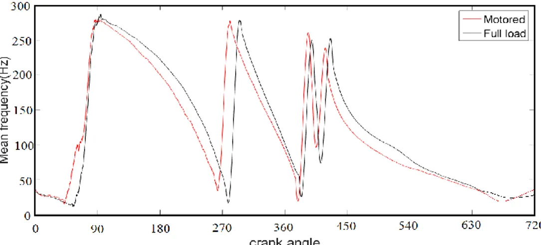
Time -frequency analysis is suitable for analysis of signals having slow frequency changes such as those generated during engine ramp down, whereas wavelet analysis is more suited for fast frequency changes such as those generated during rattle [16]. Higher time resolution at higher frequencies makes it possible to resolve short consecutive events using wavelet transformation.

2.3 Experiments

Several experiments were conducted on the test engine that is commonly used in case of small commercial vehicles. The fuel injection methodology used is a dual injection type having pre and main injection periods before piston reaches top dead center position during compression stroke. The amount of fuel injected during pre-injection period is denoted as Q pre, whereas the amount injected during main injection period is represented by Q Main. Instants

at which these injections start were defined by crank angle positions denoted by SOI pre & SOI main respectively. Fuel

is injected inside cylinders through a common rail system at injection pressure P rail that is expressed in Bars. Tests

were conducted at motored as well as full load conditions by varying various crank angle positions at which fuel is injected as shown in table no 2.1. The main aim of present activity was to analyze noise emissions from engine at different locations by changing the positioning of microphone.

2.4 Results and discussions

Diesel engine acoustics emissions contains rich information about working conditions of engine [17]. In order to analyze noise emissions at various locations, a grid was built around the test engine to change the location of microphone. Particular attention was focused on three positions marked A, B, C as depicted in figure no 2.1. Figure no 2.2,2.3 shows recorded noise emissions at three chosen locations under full load conditions. It can be observed that all traces have low frequency oscillations related to firing frequency of engine. Position C is characterized by high frequency oscillations around 360°crank angle position due to onset of combustion events. Such a trend was not visible in signals acquired at position A and B.

Figure no 2.1-Three positions to acquire noise emissions

Figure no 2.2-Noise emissions at 1600 RPM,100% load Figure no 2.3-Noise emissions at 2000 RPM,100% load

Position B was next investigated to see if any information could be extracted regarding intake flow noise. Figure no 2.4, 2.5 shows plot of intake pressures acquired at this positon. Absence of any noticeable changes in signals acquired shows that acoustic signals were least affected by load values.

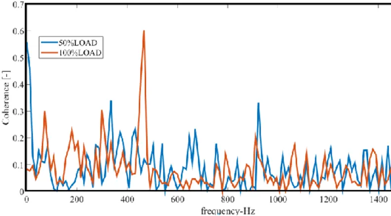
Figure no 2.4 -Intake pressure at 1600 RPM,80% load Figure no 2.5-Intake pressure at 1600 RPM,100% load Further coherence function was used for analysis of signals. This function which is denoted as a normalized function that may be defined as the ratio between the square of cross power spectral densities of input and output signals to the product of the power spectral density (PSD) of individual signals. The value of this function varies from zero to unity.

Chapter 2 Methodology for condition monitoring in engines

Figure no 2.6, 2.7 shows plot of coherence functions between intake pressure and noise radiated from engine at location B were computed using a Hanning window of length 1/6th of engine cycle. It may be observed that a close relationship exists between the two signals in frequency range [50Hz-400Hz] irrespective of load values. Such a band in which intake pressure signals are closely correlated with noise emissions is dependent on engine speed. In this frequency band, gas exchange process may be considered as a major contributor towards overall noise emissions.

Figure no 2.6 -Coherence between cylinder pressure and intake pressure signals (1600RPM)

Figure no 2.7-Coherence between cylinder pressure and intake pressure signals (2000RPM)

The noise emissions at location C were filtered in the above mentioned frequency range and compared with those of unfiltered noise emissions at location B as shown in figure no 2.8, 2.9. A close correlation between two signals shows the selected frequency band was properly chosen.

Figure no 2.8-Comparison between signals (1600RPM-100%load) Figure no 2.9-Comparison between signals (2000 RPM-100%load)