Contents lists available atScienceDirect
Energy Policy
journal homepage:www.elsevier.com/locate/enpol
An analysis of a forward capacity market with long-term contracts
Pradyumna C. Bhagwat
a,b,⁎, Anna Marcheselli
a,c, Jörn C. Richstein
a,d, Emile J.L. Chappin
a,
Laurens J. De Vries
aaFaculty of Technology, Policy and Management, Delft University of Technology, Jaffalaan 5, 2628 BX Delft, The Netherlands bFlorence School of Regulation, RSCAS, European University Institute, Il Casale, Via Boccaccio 121, 50133 Florence, Italy cFacoltà di Ingegneria Industriale e dell’Informazione, Politecnico di Milano, Via Raffaele Lambruschini, 15, 20156 Milano, Italy dDIW Berlin, Mohrenstraße 58, 10117 Berlin, Germany
A R T I C L E I N F O
Keywords: Adequacy policy Agent-based modeling Capacity markets Capacity mechanisms Electricity market Security of supplyA B S T R A C T
We analyze the effectiveness of a forward capacity market (FCM) with long-term contracts in an electricity market in the presence of a growing share of renewable energy. An agent-based model is used for this analysis. Capacity markets can compensate for the deteriorating incentive to invest in controllable power plants when the share of variable renewable energy sources grows, but may create volatile prices themselves. Capacity markets with long-term contracts have been developed, e.g. in the UK, to stabilize capacity prices. In our analysis, a FCM is effective in providing the required adequacy level and leads to lower cost to consumers and more stable capacity prices, as compared to a yearly capacity market. In case of a demand shock, a FCM may develop an investment cycle, but it still maintains security of supply. Its main effect on the power plant portfolio is more investment in peak plant.
1. Introduction
We analyze the effectiveness of a forward capacity market (FCM) in the presence of a growing share of intermittent renewable energy sources in the generation mix. We implement a representation of a FCM based on the United Kingdom's capacity market design in the “EMLab-Generation” agent-based model for this analysis.
Adequacy concerns arising from the growing share of intermittent renewable energy (cf.Nicolosi and Fürsch, 2009;Steggals et al., 2011), along with concerns about market failure due to imperfections (Cramton et al., 2013; Joskow, 2008a, 2006), have led to the im-plementation of a capacity market in the United Kingdom (UK) (UK Parliament, 2013). After much deliberation, the design for the capacity market wasfinalized in 2014. The UK chose a forward capacity market (FCM), characterized by long-term contracts for new generation capa-city. The design of the capacity market is defined by the Electricity Capacity Regulations 2014 (DECC, 2014a) and the Capacity Market Rules (DECC, 2014b). Thefirst capacity auction took place in December 2014. The expectation was that it would improve generation adequacy by providing a more stable investment signal, thus lowering investment risk.
Market participants’ decisions regarding investment in new power generation assets and with respect to decommissioning existing assets
are characterized by bounded rationality, as they are limited by their current information and therefore their forecasts are inevitably im-perfect (Simon, 1986). The market participants’ imperfect knowledge of the future can be expected to lead to suboptimal results in terms of generation investments and decommissioning. This may affect the ef-fectiveness of capacity markets in reaching public policy goals such as generation adequacy. Our analysis considers the impact of uncertainty, imperfect (myopic) investment behavior and path dependence on the performance of a forward capacity market (FCM). We analyze the ef-fectiveness of the forward capacity market under different demand growth scenarios and design considerations.
In order to understand the impact of a FCM, we compare a FCM's performance with that of a yearly capacity market design (YCM), ex-tending our earlier work in thisfield (Bhagwat et al., 2017b, 2017a). We base the YCM design in our analysis on the NYISO-ICAP1market because this is an example of a successful yearly capacity market and has a relatively simple design.
Several types of computer models have been used to study genera-tion investment in the electricity market. A classificagenera-tion of different electricity market modeling approaches is provided byVentosa et al. (2005).Boomsma et al. (2012)andFuss et al. (2012)use a real option approach in to study investment in renewable generation capacity under uncertainty. Hobbs (1995) uses a mixed integer linear
http://dx.doi.org/10.1016/j.enpol.2017.09.037
Received 31 May 2017; Received in revised form 18 September 2017; Accepted 19 September 2017
⁎Corresponding author at:Florence School of Regulation, RSCAS, European University Institute, Il Casale, Via Boccaccio 121, 50133 Florence, Italy
E-mail address:[email protected](P.C. Bhagwat).
1NYISO-ICAP: New York Independent System Operator– Installed Capacity market.
Available online 02 October 2017
0301-4215/ © 2017 The Author(s). Published by Elsevier Ltd. This is an open access article under the CC BY license (http://creativecommons.org/licenses/BY/4.0/).
programming approach to study generation investment under perfect conditions.Eager et al. (2012)use a system dynamics approach to study investment in thermal generation capacity in markets with high wind penetration. In this model, the investment decision are based on net present value and a value at risk criterion to account for uncertainty. Bunn and Oliveira (2008)use an agent-based computational model that is based on game theory to study the impact of market interventions on the strategic evolution of electricity markets.Powell et al. (2012) pre-sent an approximate dynamic programming model to study long-term generation investment under uncertainty.Botterud et al. (2002)use a dynamic simulation model to analyze investment under uncertainty over the long-term. None of these studies, however, considered the impact of a capacity mechanism on generation investment.
Hach et al. (2014)utilize a system dynamics approach to study the effect of capacity markets on investment in generation capacity in the UK. Similarly, Cepeda and Finon (2013) use a system dynamics ap-proach to analyze impact of a forward capacity market on investment decisions in presence of a large-scale wind power development. As system dynamics is a top-down approach,Mastropietro et al. (2016)use an optimization model to analyze the impact of explicit penalties on the reliability option contracts auction.Meyer and Gore (2015)use a game-theoretical approach to study the cross-border effects of capacity me-chanisms on consumer and producer surplus.Gore et al. (2016)use an optimization model to study the short-term cross border effects of ca-pacity markets on the Finnish and the Russian markets. An optimization approach is used byDoorman et al. (2007)to study the impact of dif-ferent capacity mechanisms on generation adequacy. Elberg (2014) uses an equilibrium model for the analysis of cross-border effects of two capacity mechanisms, a strategic reserve and a capacity payment, on the investment incentive. Dahlan and Kirschen (2014) andBotterud et al. (2003)study generation investment in electricity market using an optimization approach.Ehrenmann and Smeers (2011)study impact of risk on capacity expansion using a stochastic equilibrium model. In this model investment decisions are made based on the level of risk aversion of the investor. The risk aversion is modeled using a conditional value at risk (CVaR) approach.
None of the reviewed studies considered the combined impact of uncertainty, myopic investment (boundedly rational investment beha-vior) and path dependence on the development over time of an elec-tricity market with a capacity mechanism. We do include these aspects of imperfect investor behavior in our study, as the point of a capacity mechanism is to compensate for them. We do this by implementing capacity markets as an extension of the EMLab-Generation agent-based model (De Vries et al., 2013; Richstein et al., 2015a, 2015b, 2014).2 Agent based modeling (ABM) is a bottom up approach in which actors are modeled as autonomous decision making software agents (Chappin, 2011; Van Dam et al., 2013; Farmer and Foley, 2009). The behavior of the agents – in our model: the generation companies – is based on programmed decision rules. They decide about investments in new generation capacity, dismantling of old power plants and dispatch of their generation units (De Vries et al., 2013). The simulation results emerge from the agents’ decisions.
The advantages of using ABM in modeling complex socio-technical systems are discussed (Chappin, 2011; Van Dam et al., 2013; Helbing, 2012; Weidlich and Veit, 2008). In the context of electricity markets, ABM captures the complex interactions between energy producers and a dynamic environment. No assumptions regarding the aggregate re-sponse of the system to changes in policy are needed, as the output is the consequence of the actions of the agents. Furthermore, the behavior of the agents is based on the principle of bounded rationality (as de-scribed bySimon (1986)), i.e., the decisions of the agents are limited by their current knowledge and their (imperfect) prediction of the future. The agents base their decisions on their understanding of their
environment, including other agents’ actions. The results from the model are an emergent property of the agents’ interactions with each other and their environment, thus the results typically do not follow an optimal path. This allows us to study the possible evolution of the electricity market under conditions of uncertainty, imperfect informa-tion and non-equilibrium.
Aside from the advantages of using an ABM for this analysis, the implementation of a detailed representation of capacity markets in EMLab-Generation model provides several advantages. Thefirst is that the ability to vary different design parameters (such as the installed reserve margin (IRM) requirement) of the FCM forward capacity market allows us to study the sensitivity of the design to changes in the design parameters. Secondly, it allows us to compare two different capacity market designs. Furthermore, EMLab-Generation allows us to study the effectiveness of the FCM under varying demand growth conditions, especially a situation in which the system undergoes a de-mand shock. A disadvantage of ABM is that it is time- intensive, both with respect to developing the model (in Java) and running it (it re-quires a high-performance computer cluster to conduct Monte Carlo runs that are required for this analysis). Due to the long runtime, the scope is limited. A key limitation for this purpose is the abstraction of demand into a load-duration curve, which does not allow for the re-presentation of demand elasticity or storage. This may cause more vo-latile prices and therefore exaggerate the need for a capacity me-chanism. Another drawback of this modeling approach is that traditional validation processes cannot be applied, making validation of agent-based models challenging (Louie and Carley, 2008).
We will proceed by describing the EMLab-Generation agent-based in the next section. InSection 3, the implementation of a capacity market in EMLab-Generation is presented. This is followed by the description of the scenarios and performance indicators that are used in this study in Section 4. The results are discussed inSection 5and the conclusions are summarized inSection 6.
2. The EMLab-Generation model
2.1. EMLab-Generation
The EMLab-Generation agent-based model (ABM) was developed in order to model questions that arise from the heterogeneity of the European electricity sector and the interactions between different policy instruments (De Vries et al., 2013; Richstein et al., 2015a, 2015b, 2014). The model provides insight in the simultaneous long-term im-pacts of different renewable energy, carbon emissions reduction and resource adequacy policies, and their interactions, on the electricity market.
Power generation companies are the central agents in this model. The behavior of the agents is based on the principle of bounded ra-tionality (as described bySimon (1986)), i.e., the decisions made by the agents are limited by their current knowledge and their limited un-derstanding of the future. The agents interact with each other and other agents via the electricity market and thereby change the state of the system. Consequently, the results from the model do not adhere to an optimal pathway and the model is typically not in a long-term equili-brium. Therefore, the model allows us to study the evolution of the electricity market under conditions of uncertainty, imperfect informa-tion and non-equilibrium.
In the short term, the power generation companies make decisions about bidding in the power market. Their long-term decisions concern investments in new capacity and decommissioning of power plants. The model resembles a cost-minimizing model in which investments are based on expected costs, as we did not program differences in the agents’ behavioral algorithms. The only difference between the agents develops in the state of theirfinances during the simulation: agents that made bad investment decisions have less money to invest in later years. By having multiple agents with different bank balances, the effects of
negative returns due to over investment develop more gradually than if it had been a cost-minimization model with a single investment deci-sion.
The main external drivers for change in this model are the fuel prices, electricity demand growth scenarios and policy instruments such as capacity mechanisms. The main outputs are investment behavior and its impact on electricity prices, generator cost recovery, fuel con-sumption, evolution of the supply-mix and system reliability.
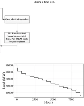
The model provides the functionality for conducting an analysis of an isolated electricity market as well as an interconnected electricity system. The representation of an interconnected system is limited to two zones with an interconnector. As the objective of this paper is to understand the evolution of the electricity market over the long-term, all scenarios consist of 40 time steps, each of which represents one year. An overview of the model activities during a time step is presented in aflowchart inFig. 1. At the start of each time step, the power gen-eration companies make annual loan payments (if any) for their power plants. In the next step, the power generation companies submit price-volume bids to the electricity market for all available power plants, after which the electricity market is cleared. Next, the companies pur-chase fuel for their power plants, pay their operation and maintenance costs and are payed for the energy they sold on the electricity market. In the last step, the power generation companies make decisions regarding investment in new capacity and dismantling of existing power plants.
A detailed description of EMLab-Generation has been presented in a report (De Vries et al., 2013), scientific literature (Bhagwat et al., 2016b; Richstein et al., 2015a, 2015b, 2014) and in a doctoral thesis (Richstein, 2015; Bhagwat, 2016). In the next section the structure of the model is described in detail followed by the input assumptions, model outcomes and model limitations. Please note that the description of the model presented in Section 2 is based on (Bhagwat, 2016; Bhagwat et al., 2017b)
2.2. Model
2.2.1. Demand
In this model, a single agent procures electricity on the behalf of all consumers. Electricity demand is represented in the form of a step-wise approximation of an empirical load-duration curve. The segments of the step function have variable numbers of hours. (SeeFig. 2.) Thus, each segment of the load duration curve has an assigned load value and a time duration, which is set as part of the initial input scenario. In each time step of the simulation, the load value for all segments is updated based on the exogenous demand growth rate. These segments are been called“load blocks” or “load levels” in literature (Wogrin et al., 2014). This approach for representing demand in electricity market models has been utilized for power system modeling since the 1950s, especially for medium and long-term models (Wogrin et al., 2014). The most important advantage of using this approach is that it allows for a
shorter run time, enabling a larger number of simulations within a practical time frame (Richstein et al., 2014). However, due to the loss of temporal relationship between load hours, short term dynamics such as ramping constraints, unplanned shutdowns, demand elasticity and load shifting by storage units cannot be modeled (Wogrin et al., 2014).
2.2.2. Electricity market clearing
The electricity market is modeled as an abstraction of an hourly power system (Richstein et al., 2014). Within each one-year time step, the electricity market is cleared for each segment of the load-duration curve. Therefore, the segment-clearing price is considered as the elec-tricity price for the corresponding hours of the particular segment. In this model the load duration curve is divided into 20 segments.
The power generation companies create price-volume bid pairs for their controllable (thermal) power plants for each segment of the load-duration curve. (Variable renewable energy generation is treated dif-ferently, as described inSection 2.2.5.) The power generation compa-nies bid their power plants into the market at their marginal cost of generation, which is determined solely by the fuel costs. The volume component of the bid is based on the capacity of the available power plants. Outages are not modeled; availability is assumed to be 100%. The supply curve for each segment is constructed by sorting the bids in ascending order by price (merit order). The electricity market is cleared at the point where demand and supply intersect. The highest accepted bid sets the electricity market-clearing price for that segment of the market. If demand exceeds supply, the clearing price is set at the value of lost load (VOLL).
2.2.3. Investment algorithm
The investment behavior of the power generation companies is based on the assumption that investors continue to invest up to the point that it is no longer profitable. In this model, power generation companies invest only in their own electricity markets thus entry into a new market is not considered.
All investments are financed using a combination of debt and equity. The power generation company considers investment in a new
Fig. 1. Stylized flowchart of the model activities during a time step.
power plant only if it has sufficient cash on hand to finance the ne-cessary equity. The power generation companies invest the equity from their cash balance, based on a user defined expected rate of return on equity. A bankfinances the debt at a user-defined interest rate. The debt is repaid as equal annual installments over the depreciation period for the power plant. In this model, the power generation company can choose between 14 power generation technologies types for making investments (SeeTable A1 in Appendix A).
Power generation companies make investment decisions sequen-tially in an iterative process. The investment decision of each power generation company affects the investment decision of the next power generation company by changing its forecast of available capacity (we assume that power generation companies have full information about investment decisions that have already been made by competitors). This iterative process stops when no participant is willing to invest further. To prevent a bias towards any particular agent, the sequence of power generation companies is determined randomly in every time step.
At the start of each investment round, each power generation company makes a forecast of the future demand and fuel prices at a point of time in the future (reference year) by extrapolating the growth rate of demand from the past. The expected fuel prices are used to calculate the marginal variable costs of all power plants that are ex-pected to be available in the reference year. These may be new power plants that have been announced or existing power plants that are within their expected life span in the reference year. The future elec-tricity price for each segment is estimated by creating a merit order of the available power plants for each segment of the load duration curve. Next, the power generation companies compare the outcomes of investing in different power generation technology options available. They calculate the expected cashflow in the reference year for a power plant of each power generation technology under consideration. The expected cashflow is calculated by subtracting the fixed costs of the given power plant from its expected electricity market earnings. The expected earnings from the electricity market are calculated based on the power plant's expected running hours, the electricity prices and the variable costs (calculated based on expected fuel prices) in those hours of the reference year. The expected running hours of a power plant are calculated by comparing the expected electricity prices for each seg-ment and the expected variable cost of the power plant under con-sideration. If the variable cost is lower than the electricity price, the power plant is assumed to have cleared the market in that segment. Therefore the power plant is assumed to have run for all hours of the given segment.
The expected cash flow value for each power plant under con-sideration is used to calculate the specific net present value (NPV) per MW, over the construction period and the power plant's expected ser-vice period. A weighted average cost of capital (WACC) is used as the interest for the NPV calculation. The power generation company invests in the power generation technology with the highest positive specific NPV. If all NPVs are negative then no investment is made.
2.2.4. Decommissioning power plants
The power generation companies base their dismantling decisions mainly on the operational profitability of each power plant. In each time step, the power generation companies iterate through their set of power plants in order to make decommissioning decisions. For each power plant, the aggregated cashflow over the previous years is cal-culated. The time horizon (in years) for this look back is a user-defined value. If the cashflow of the power plant is negative, the power gen-eration company makes a forecast of the cashflow for the coming year. If this forecasted cash flow is also negative, the power plant is de-commissioned. In order to simulate the rising costs of old power plants, the operation and maintenance costs of power plants that are active beyond their operational age are increased year-on-year. This ensures that all old power plants are eventually dismantled (depending on
market conditions).
2.2.5. Intermittency of renewables
The intermittency of renewables is a short-term effect that is diffi-cult to implement in a long-term model such as EMLab-Generation, because demand is represented as a load duration curve. In this model, intermittency is approximated by varying the contribution of these technologies (availability as percentage of installed capacity) to the different segments of the load-duration curve. The segment-dependent availability is varied linearly from a large contribution to the base segments, to a very small contribution to the highest peak segment. This corresponds to the contribution of solar and wind energy to peak de-mand in Germany.
2.2.6. Renewable energy policy
The development of renewable electricity generation is im-plemented as investment by a renewable‘target investor’. If investment in renewable energy source (RES) based capacity by the competitive power generation companies is lower than the government target, the target investor will invest in additional RES capacity in order to meet the target even to the extent that the investor does not recover its costs in the market. This simulates the current subsidy-driven development of renewable energy sources.
3. Capacity markets
3.1. Overview
A capacity market is a quantity-based capacity mechanism. The desired quantity of the available generation capacity is administratively set and the market decides the price. In a capacity market, consumers, or agents on their behalf, are obligated to purchase capacity credits equivalent to the sum of their expected peak consumption plus a re-serve margin through a process of auctions (Agency for the Cooperation of Energy Regulators (ACER), 2013; Cramton and Ockenfels, 2012; Cramton et al., 2013; Creti and Fabra, 2003; Iychettira, 2013; Stoft, 2002; Wen et al., 2004). The additional revenues from the capacity market are intended to help power plants to recover theirfixed costs (Joskow, 2008a, 2008b, 2006; Shanker, 2003).
A capacity market is expected to provide a stronger and earlier in-vestment signal than wholesale electricity prices and thus improve adequacy. It can therefore be used to compensate for under investment that might occur as a result of electricity price risk. This price risk is expected to increase as the shares of solar and wind energy grow. Demand response and electric energy storage, on the other hand, would dampen prices. However, the cost of large-scale energy storage cur-rently still is too high (Zakeri and Syri, 2015) while the potential for demand response appears limited. Because our model is not capable of including demand response and storage, due to the use of a load-duration curve, it represents a pessimistic scenario. If electrical energy storage becomes substantially cheaper and demand response achieves a significant market share, the need for a capacity mechanism may be lessened.
3.2. The forward capacity market design3
We based the design of the forward capacity market with long-term contracts on the recently implemented UK capacity market. In this section, we describe the key design elements of the UK capacity market and its implementation in the EMLab-Generation model. A forward
3Please note that the forward capacity market was implemented by extending the
yearly capacity market model (also described in Section 3.3 of this paper) that was de-veloped as part of our earlier studies presented in (Bhagwat, 2016; Bhagwat et al., 2017; Iychettira, 2013).
market means that the capacity that clears the market in the current year needs to be available in a future reference year, in this case four years from the current year. Therefore, any generation unit that is ex-pected to be available in the reference year, whether existing or under construction, can participate in the capacity market. Moreover, in the UK capacity market design, new and refurbished capacity that clears the market is provided with a long-term contract. A detailed description of all the rules of the capacity market is available inDECC (2014a).
On the supply side, the most significant element of the UK capacity market design is the heterogeneity of contract lengths. Power plants that clear the capacity auction and are new or less than four years from completion, are awarded 15-year contracts. Existing power plants that clear the four-year ahead capacity market are awarded a one-year contract. Plants that are being refurbished may obtain contracts of 3-year duration. Capacity that is awarded long-term contracts is ineligible for participation in the capacity market for the duration of the contract. Renewable energy capacity that receives renewable policy support is also ineligible to participate on the capacity market.
In the capacity market module of our model, the power producers submit price (in€/MW per year) - capacity (in MW) bids for each eli-gible power plant to the capacity market. The capacity component of a power plant's bid is determined by its capacity that is available during peak load. Existing and new power plants bid differently. A marginal cost-based approach is used for existing power plants. Per generation unit, the owner calculates the expected revenue from the electricity market. If the generation unit is expected to earn adequate revenues from the electricity market to cover its fixed operations and main-tenance costs (in other words, its costs of staying online), the bid price is set to zero and the plant becomes a pure price taker. Units that are not expected to make adequate revenues from the energy market to cover theirfixed costs of remaining online bid the difference between thefixed costs and the expected electricity market revenue, which is the minimum revenue that would be required to remain online. The bid price of plant that is new or under construction is set at itsfixed op-erating cost, which is the minimum revenue that such a power plant would require to remain online without earning any revenue from the wholesale electricity market.
Power plants that are have a long-term capacity contract do not participate in the capacity market for the duration of the contract. At the end of the long-term contract period, these power plants are al-lowed to participate in the capacity market as existing capacity that is eligible for one-year contracts.
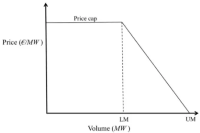
On the demand side, a sloping demand curve is utilized (Cramton and Stoft, 2005; DECC, 2014b; Hobbs et al., 2007; NYISO, 2013a, 2013b;Pfeifenberger et al., 2009). The system operator purchases ca-pacity from the generation companies and passes the cost along to the consumers. The regulator sets the values of the installed reserve margin (IRM), the capacity market price cap and the slope of the demand curve. The capacity market price cap represents the consumers’ (or the regulator's) maximum willingness to pay for capacity. The demand re-quirement is reduced based the volume of long-term capacity contracts and on the contribution of renewables to peak load.
A forward market means that the capacity that clears the market in the current year needs to be available in a future year. The absolute value of the demand requirement (Dr) in MW for the current auction is based on four variables: the installed reserve margin (r), the expected peak demand (Dpeak) for the forward year, which is forecasted by ex-trapolating past peak demand values, the total capacity that already has long-term capacity contracts (CLT) and the total peak available capacity of renewable generation with renewable energy policy support (CRES). The following equation describes the calculation of the demand re-quirement value:
= − − × +
Dr (Dpeak CLT CRES) (1 r) (1)
The demand target is calculated for the entire zone without con-sidering locational and transmission constrains within a single zone.
A sloping demand curve is modeled for the capacity market like in the NYISO-ICAP and PJM-RPM capacity markets. These markets im-plement sloping demand curves to provide more predictable revenues to generators and to lower consumer costs by reducing price volatility (Hobbs et al., 2007). When a sloping demand curve is implemented, changes in the offered volume of capacity result in small price changes, thus stabilizing capacity market prices (Pfeifenberger et al., 2009). As is illustrated inFig. 3, the sloping demand curve consists of two lines: a horizontal line at the capacity market price cap (Pc) and a sloping line intersecting the horizontal line and the X– axis. The slope and position of the sloped line are dependent upon three user-defined variables, namely, the demand requirement (Dr), the lower margin (lm) and the upper margin (um). The lower and upper margins are administratively set maximum flexibility boundaries above and below the IRM. The sloping line intersects the horizontal line at Point (X = LM, Y = Pc). The slope of the line is calculated using the following equation
= − m P LM UM c (2) = × + + UM Dpeak (1 r um) (3) = × + − LM Dpeak (1 r lm) (4)
The capacity market clearing algorithm is modeled as a uniform price auction. The bids submitted by the power producers are sorted in ascending order by price and cleared against the sloping demand curve. In our model, two types of contracts are offered to power plants that clear the capacity market to account for the heterogeneity of contract lengths. Existing capacity without a long-term contract is awarded a one-year contract. Capacity that is new or under construction and ex-pected to be functional in or before the forward year is awarded a long-term contract at the auction clearing price. The forward period is four years and the long-term contract length is chosen to be 15 years, like in the UK. Since plant refurbishment is not modeled, we do not consider this contract option in our model.
After the market is cleared, existing units that clear the capacity market (receive a one-year contract) are paid the current capacity market-clearing price. Newly built or under-construction capacity that clears the market (is awarded a long-term contract) receives payments for the period of the long-term contract fixed at the current year's market-clearing price. All remaining power plants with long-term contracts are also remunerated based on their contract price.
3.3. The yearly capacity market
We compare the performance of the long-term capacity market with that of a yearly capacity market module (YCM). The YCM was devel-oped as part of our earlier studies presented in Iychettira (2013), Bhagwat (2016)andBhagwat et al. (2017b, 2017a). The yearly capa-city market module in EMLab-Generation is modeled with a few
simplifications after the NYISO-ICAP model. The NYISO market was chosen for its relatively simple design. Moreover, it was one of thefirst capacity markets to be established in the United States and may be considered as an example of a capacity market that is arguably meeting its policy goals. Moreover, it is projected that no new resource re-quirements would be necessary in NYISO region till 2018 (Newell et al., 2009).
In the NYISO-ICAP, generators offer unforced capacity4 (UCAP) (NYISO, 2013a, 2013b) in a series of auctions. The auctions are con-ducted annually for the following year. The ISO contracts capacity on behalf of load serving entities (LSEs); thus, consumers participate au-tomatically. A sloping demand curve is utilized. Consumers are pro-vided opportunity to correct their positions during the year via the monthly spot auctions and capability period auctions. In each year there are two capability periods, summer capability period (May 1st–Oct 31st) and winter capability period (Nov 1st–April 30th) (Bhagwat et al., 2016a; NYISO, 2014). The LSEs are obligated to pur-chase capacity credits equivalent to the minimum unforced capacity (UCAP) assigned to them (Harvey, 2005; NYISO, 2013a, 2013b). The value of unforced capacity is calculated as the product of the Installed Reserve Margin (IRM) and the forecasted peak demand (NYISO, 2013a). The regulator calculates the IRM so as to achieve a loss of load expectation of once in 10 years. NYISO allows bilateral capacity con-tracts and imports to participate on the capacity market subject to certain rules and regulations. A detailed description of the market rules is given in (NYISO, 2013a; Spees et al., 2013).
In the yearly capacity market that is modeled in EMLab-Generation, the capacity for the coming year is traded in a single annual auction and is administered by an agent called the capacity market regulator. The user sets the IRM, capacity market price cap and parameters for gen-erating the slope of the demand curve.
The regulator calculates the demand requirement (Dr) for the cur-rent year based on the IRM (r) and the expected peak demand (Dpeak). Expected peak demand is forecast by extrapolating past values of peak demand using geometric trend regression over the past four years. The demand requirement is calculated with the following equation.
= × +
Dr Dpeak (1 r) (5)
The sloping demand curve for the yearly capacity market is modeled similarly to the forward capacity market as described in the earlier section.
The supply curve is based on the Price (€/MW) – Volume (MW) bid pairs submitted by the power generators for each of their active gen-eration units. The agents calculate the volume component of their bids for a given year as the generation capacity of the given unit that is available in the peak segment of the load-duration curve. A marginal cost-based approach is used to calculate the bid price. For each of power plant, the power producers calculate the expected revenues from the electricity market. If the generation unit is expected to earn ade-quate revenues from the electricity market to cover itsfixed operating and maintenance costs (in other words, its costs of staying online), the bid price is set to zero, as no additional revenue from the capacity market is required to remain operational. Units that are not expected to make adequate revenues from the energy market to cover theirfixed costs of remaining online, bid the difference between the fixed costs and the expected electricity market revenue, the minimum revenue that would be required to remain online.
The yearly capacity market-clearing algorithm is based on the concept of uniform price clearing. The bids submitted by the power producers are sorted in ascending order by price and cleared against the above-described sloping demand curve. The units that clear the capa-city market are paid the market-clearing price. While making
investment and dismantling decisions, the power generators take into account the expected revenues from the capacity market.
4. Scenarios and indicators
All scenarios are run over a time horizon of 40 years, 120 times in a Monte Carlo fashion with identical initial conditions. The initial supply mix is roughly based on theEurelectric (2012)data for the UK. The renewable energy growth trends in all the scenarios are modeled based on UK's national renewable action plan (Beurskens et al., 2011; DECC, 2010) up to year 2020 and thereafter they follow the 80% pathway of the European Climate foundation's Roadmap 2050 projections (European Climate Foundation, 2010). The load duration curve is based on the ENTSO-E hourly demand data for the year 2014 for UK.
The fuel prices and demand growth are uncertain. The uncertainty of these parameters is created using a triangular trend distribution. The natural gas and coal price trends are based on fuel projects of the UK Department of Energy and Climate Change (Department of Energy and Climate Change, 2012) and extrapolated beyond 2035. The price trends for biomass (based on Faaij (2006)) and uranium are modeled sto-chastically using a triangular distribution. The average annual demand growth is 1%.
Depending upon the nature and location of the load, the estimate of value of lost load can vary significantly as observed from literature (Anderson and Taylor, 1986; Baarsma and Hop, 2009; Leahy and Tol, 2011; Linares and Rey, 2013; Pachauri et al., 2011; Wilks and Bloemhof, 2005). In this modeling, VOLL was chosen at the relatively low level of 2000€/MWh. We also chose this level to take into account demandflexibility that might occur during periods of high prices.
We consider an isolated electricity market without interconnection and with four similar generation companies. The baseline scenario BL consists of an energy-only market (no capacity market). The scenario LTCC consists of an electricity market with a four-year forward capacity market implemented in the system. New and under construction ca-pacity that clears the caca-pacity market is awarded a 15-year long-term contract while existing capacity is awarded a one-year contract. The scenarioSTCC consists of an electricity market with a yearly capacity market in which the capacity market is cleared for the coming year. In both the LTCC and STCC scenarios, the capacity market price cap is set at 95 k€/MW. This value is based on the price cap used in the UK ca-pacity market. The lower and upper margins of the sloping demand curve are set at 3.5%. The installed reserve margin (IRM) requirement is set at 10% of peak demand.
The following indicators are used for evaluating the performance of the capacity markets:
•
The average electricity price (€/MWh): the average electricity price over an entire run.•
The number of shortage hours (hours/year): the average number of hours per year with scarcity prices, averaged over all years and all Monte Carlo“runs” of a scenario.•
The supply ratio (MW/MW): the ratio of available supply over peak demand.•
The average cost to consumers of the capacity market (€/MWh): the cost incurred by consumers for contracting the mandated capacity credits from the capacity market, divided by the total units (MWh) of electricity consumed.•
The total average cost to consumers5 (€/MWh): the sum of the electricity price, the cost from the capacity market and cost of re-newable policy (if applicable) per unit of electricity consumed.4Unforced capacity is defined as the amount of electricity generated by a power
generator after accounting for any outages (NYISO, 2013a, 2013b).
5Note that this includes the cost of outages, because in our model the electricity price
5. Results and analysis
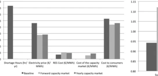
In this section, the model results are analyzed.Fig. 4presents an overview. The results are also presented in a numerical form in Table A2 of theAppendix A.
5.1. Performance of the forward capacity market
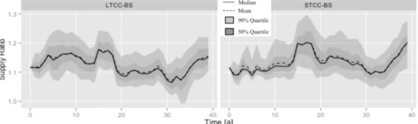
In this section, results from the scenario with a forward capacity market (LTCC) are compared with the baseline scenario (BL). The presence of a capacity market leads to an average supply ratio of 1.12 (a reserve margin of 12%). This value is two percentage points higher than the adequacy target of 10%, but it is within the 3.5% point upper boundary. This overshoot can be attributed to the configuration (price cap and slope) of the demand curve used in this analysis. The capacity market clears at a level where it becomes economically viable for excess idle capacity above the targeted IRM to remain available. On an average, the forward capacity market clears at a price of 32,850€/MW. The implementation of a forward capacity market increases the reserve margin substantially and reduces most of the investment cycles that we see in the baseline scenario, but a smaller and slower invest-ment cycle is still present. SeeFig. 5. In thisfigure and the ones like it, the mean is indicated with a solid line, the average with a dashed line, the 50% confidence interval with a dark grey area and the 90% con-fidence interval with the lightly shaded area. The difference with an yearly capacity market, in which capacity contracts last only a year, is not big, however; in fact, the yearly capacity market seems to provide a more stable reserve margin than the long-term capacity market.
Early in the model runs, the power producers invest in new capacity
because they expect sufficient returns from the capacity market. Due to its short construction time and low capital cost, OCGT is the preferred technology type for investment (See Fig. 6.). This new-built and/or under construction capacity clears the capacity market and is awarded long-term contracts, as it requires the lowest capacity price to remain online, even if it has little or no revenue from the electricity market. This capacity either operates during peak hours or remains idle alto-gether. The increase in capacity with long-term contracts leads to a reduction in the remaining capacity requirement (as the capacity re-quirement is reduced by the capacity having long-term contracts). However, these new‘peaker’ plants are low in the merit order. Conse-quently, the existing supply function is extended with the new‘peaker’ plants and the capacity market clearing prices are depressed, making investment in new capacity less attractive. The revenues of existing power plants that receive annual capacity contracts also decline,
Fig. 4. Performance overview of the three market designs.
Fig. 5. The supply ratio in scenarios without a capacity market (left), with a forward capacity market (center) and a yearly capacity market (right).
Fig. 6. The average volume of OCGT capacity awarded with long-term contracts in the capacity auction.
leading to dismantlement of power plants that do not receive adequate revenues. Because of the time delay in the market parties’ responses, an investment cycle develops.
Because the IRM is set well above the real need for capacity, the capacity market stimulates power generators to invest in generation capacity that either remains idle or runs rarely. (This is partly a model
artifact, as we do not model generator outages.) Therefore, investment in OCGT technology with lowest capital cost becomes the preferred choice. The average volume of installed OCGT capacity increases from 6.1 GW in the baseline scenario to 14.7 GW in the forward capacity market (Fig. 7). The presence of a forward capacity market does not
Fig. 7. The average volume of installed capacity of OCGT in a scenario without (left) and with a forward capacity market (right).
Fig. 8. Electricity price in scenario without (left) and with (right) forward capacity market.
Fig. 9. Average electricity price difference between scenarios with a yearly capacity market (STCC) and a forward capacity market (LTCC).
Fig. 10. Capacity prices in scenario with a forward capacity market (left) and with a yearly capacity market (right).
affects the development of nuclear capacity in the system, because the remuneration from the capacity market does not add sufficient revenue for new nuclear power plants to recover their costs.
In the presence of a forward capacity market, the high reserve margin causes the number of shortage hours to decline to almost nil. As a result, the average wholesale electricity price declines by 33% as compared to the baseline scenario. A significant reduction in price volatility is also observed due to the overcapacity (Fig. 8). As is ob-served inFig. 4, the reduction in shortage hours leads to an increase in the cost of renewable energy subsidy. The cost to consumers of the capacity market is 5.7€/MWh. However, the savings from reduction in shortage hours is large enough to compensate for these additional costs. In the presence of a forward capacity market, the overall cost to con-sumers declines by 15% on average as compared to the baseline sce-nario. We observe that on average, the annual generation increases by 234 GWh in the scenario with a forward capacity market as compared
Fig. 12. Supply ratios in a scenario with a forward capacity market (left) and a yearly capacity market (right), in the presence of a demand shock.
Fig. 13. Capacity market prices in scenario with a forward capacity market (left) and a yearly capacity market (right), in the presence of a demand shock.
Table 1
Scenario settings for the sensitivity analysis. Scenario Capacity market
cap (k€/MW) Upper margin (%) Lower margin (%) Long-term contract length (years) 1 75 3.5 3.5 15 2 95 3 105 4 95 1.5 1.5 5 3.5 3.5 6 5.5 5.5 7 3.5 3.5 10 8 15 9 20
Fig. 14. Standard deviation of forward capacity market prices in scenarios with different price caps.
Fig. 15. Price uncertainty of forward capacity market prices in scenarios with different demand slopes.
to the baseline scenario, which leads to elimination of the shortage hours in scenario LTCC.
5.2. Comparison with the yearly capacity market
In this section, we compare the forward capacity market (scenario LTCC) with a yearly capacity market (scenario STCC). Both capacity market designs are able to provide the mandated installed reserve margins (IRM) levels. The average supply ratios in both scenarios are comparable (1.12 in LTCC and 1.125 in STCC). A similar reduction in shortage hours is observed in both scenarios (LTCC and STCC). The average electricity prices in both the scenarios are also comparable (prices in a scenario with a forward capacity market are marginally (1%) lower than that in the yearly capacity market).Fig. 9illustrates the difference between average electricity prices in the two scenarios. The maximum difference between the prices is less than 2 €/MWh.
The capacity market prices in the yearly capacity market are more volatile than those in the forward capacity market (Fig. 10). This can be attributed to the short-term nature of the yearly capacity market. Consequently, the average cost of the capacity market to the consumers is significantly higher in a scenario with a yearly capacity market (8.6 €/MWh) than with a forward capacity market (5.7 €/MWh). This translates into a 4% higher total cost to consumers in the scenario with a yearly capacity market as compared to a scenario with a forward capacity market. The total cost to consumer in a scenario with a FCM is 53.7€/MWh while in the one with a YCM is 56.1 €/MWh.
5.3. The effectiveness of a forward capacity market in the event of a demand shock
While both capacity market designs perform well in scenarios with generally smooth demand growth, we also tested how well they stand up to a sudden shock like the drop in electricity demand in Europe in the aftermath of the 2008financial crises. We apply this scenario to both the short-term and the long-term capacity markets. The average demand growth trend (over all 120 Monte Carlo runs) is 1.5% for the first 14 years of the simulation. Then there is a sudden drop in demand. Subsequently, the average growth rate is zero for several years, after which it returns to 1.5% in the last 11 years of the simulation. The demand growth trajectory including the 50% and 90% confidence in-tervals is presented in Fig. 11. The above described demand growth trajectory also was used in our earlier research (Bhagwat et al., 2017a). The drop in the demand leads to an investment cycle, both in a forward and an yearly capacity market. In case of a forward capacity market (FCM), the dip in demand leads to a spike in the supply ratio, which proceeds to decline gradually as the system adjusts to the zero growth level. The supply ratio stabilizes at the 10% IRM level. As de-mand growth picks up again, the capacity market price rises, which is followed by investment in new generation capacity. The total cost to
consumers in a demand shock scenario with an FCM is 55.1€/MWh. In the case of an yearly capacity market (YCM), the capacity clearing price is more sensitive to the demand growth changes. The demand shock leads to overcapacity and a steep drop in the capacity price. As demand growth does not rebound, we see a gradual dis-mantling of unprofitable power plants over the next years. When de-mand starts to grow again, this causes a price spike in the capacity market as the reserve margin is significantly diminished due to the dismantling. This reinforces the investment cycle. The total cost to consumers in a demand shock scenario with an YCM is 57.3€/MWh.
As the capacity is traded year-ahead only, significantly higher price volatility is observed in the yearly capacity market than in the forward capacity market. As the decision regarding the decommissioning of power plants is based on their profitability, the price volatility provides these power plants with adequate revenues to break-even and remain in the system for a longer time, thus decommissioning of power plants is slower with a yearly capacity market as compared to a forward capacity market. This results in an overall higher reserve margin in a region with a yearly capacity market during the period with no demand growth (See Figs. 12 and 13). When we compare the results of both scenarios, we find that while both capacity markets experience an investment cycle but both continue to provide adequacy.
5.4. Sensitivity analysis
In this section, we study the sensitivity of the forward capacity market (FCM) to different design parameters. The variations to the design parameters used in this analysis are presented inTable 1.
5.4.1. The capacity market price cap
As the capacity market price cap (the maximum willingness to pay for capacity) is set by the regulator, we tested the model's sensitivity to this parameter. The model was run with capacity market price cap values between 75 k€/MW and 115 k€/MW in increments of 20 k €/MW. SeeTable 1, Scenarios 1–3. All other parameters in the scenarios were kept the same as in the LTCC scenario. The forward capacity market design does not exhibit a strong sensitivity to change in the value of capacity market price cap in terms of costs or supply ratios. The differences in the average cost to consumers and average supply ratio values are negligible.
Considering the development of the capacity clearing price trends over the entire simulation run, we observe that a lower capacity market price cap reduses the price uncertainty in the capacity market. This can be observed from the standard deviation values inFig. 14. An increase in the price cap would effectively make the slope of the capacity market demand curve steeper, making the capacity price more volatile. This result conforms to the theory that a vertical or steep demand curve leads to more volatile prices (Hobbs et al., 2007).
Fig. 16. Price uncertainty of capacity market prices in scenarios with differing long-term contract periods.
5.4.2. The slope of the capacity demand curve
We also tested the sensitivity of the forward capacity market to three different slope configurations by varying the upper and lower margins of the capacity demand curve. SeeTable 1: Scenarios 4–6.
The performance of the forward capacity market, in terms of the supply ratio and cost of capacity, is not very sensitive to changes in slope of the capacity demand curve. However, a steeper demand curve causes the capacity market prices to be more volatile (Fig. 15). This indicates that a sloping demand curve is effective in reducing price uncertainty in the capacity market. As mentioned above, this observa-tion corresponds with theoretically expectaobserva-tions.
5.5. Contract duration
We vary the contract length from 10 to 20 years in steps of 5 years. SeeTable 1: Scenarios 7–9. As explained inSection 5.1, the generation capacity that obtains long-term contracts is mostly OCGT, as it has the lowest cost of remaining online, even with little or no revenue from the electricity market. This leads to reduction of the capacity requirement in the FCM and consequently to lower capacity clearing prices. Longer contract duration leads to longer periods with lower capacity market prices. This translates into a lower average capacity market clearing price and a reduction in the price uncertainty on the capacity market. SeeFig. 16.
However, it does not lead to a reduction in the overall cost to consumer from the capacity market. The cost savings from to the lower capacity market price are not very large, while the longer contract duration entails remunerating this capacity for a longer period, which adds to the cost to consumers. Therefore, on an average, the overall cost to consumer from the capacity market is not affected significantly by the duration of the long-term contracts.
6. Model limitations
As was described in earlier work (Bhagwat et al., 2017b, 2017a, 2016b, 2014), we do not consider market power or strategic behavior of power producers in neither the electricity market nor the capacity markets. Therefore, the dynamics that may arise due to strategic be-havior of various market participants, e.g. during shortages, are not captured. The impacts of demand response and storage on the long-term development of the electricity market are left out of the scope of this study. However, they have a stabilizing impact on electricity prices and may reduce the need for a capacity mechanism. As EMLab-Gen-eration model was developed to study the long-term development of the electricity market, short-term effects such as unscheduled shutdowns of power plants are not modeled. These assumptions, along with the segmented nature of the load-duration curve, make the short-term dy-namics less precise. Among others, they explain the overshoot in ade-quacy that is observed in the model results. Finally, mothballing of power-plants has not been modeled. Such a provision could be attrac-tive for generation companies during periods of uncertainty. In the context of this model it may dampen investment cycles.
7. Conclusions
We present a model of a forward capacity market with long-term contracts that is based on the UK capacity market design in a system with a growing share of renewable energy. We compare this forward capacity market with a yearly capacity market that is based on the NYISO-ICAP design. The model represents a pessimistic scenario in which electrical energy storage and demand response do not gain a significant market share.
The implementation of a forward capacity market reduces the in-vestment cycles observed in our baseline energy-only scenario. However, a smaller and slower investment cycle still exists. A forward capacity market leads to a significantly higher supply ratio, substantial reduction in the number of shortage hours and lower overall cost to consumers as compared to a baseline energy-only market, but its per-formance is not significantly better than that of a short-term (yearly) capacity market. To the contrary, both without and with a demand shock, the capacity market with long-term contracts exhibited a higher risk of failing to maintain system adequacy. The reason is that the forward capacity market responds a little slower to changes as com-pared to a yearly capacity market.
On the other hand, the forward capacity market reduces overall consumer cost, as compared to a scenario with a yearly capacity market, because the capacity price in a forward capacity market is less volatile and slightly lower on average than in a yearly capacity market. Like the yearly capacity market, the forward capacity market increases investment in low-cost peak generation capacity as compared to an energy-only market.
In accordance with the literature, we found that a gentler slope of the capacity demand function (larger upper and lower margins) reduces capacity price uncertainty. The performance of the capacity market does not change significantly if the contract duration is extended be-yond ten years. Our model was run with perfectly inelastic demand. Demand response and electric energy storage could significantly dampen electricity prices and thereby reduce the need for a capacity market, but as their shares are not large and their economic potential is uncertain, our model reflects the current state of electricity markets. Future extensions could include plant outages and the impact of de-mand response, energy storage and cross-border exchanges on the need for, and the performance of, a capacity market.
Acknowledgments
Pradyumna Bhagwat and Jörn C. Richstein have been awarded the Erasmus Mundus Joint Doctorate Fellowship in Sustainable Energy Technologies and Strategies (SETS) hosted by the Universidad Pontificia Comillas, Spain; the Royal Institute of Technology, Sweden; and Delft University of Technology, The Netherlands. The authors would like to express their gratitude towards all partner institutions within the program as well as the European Commission for their support.
References
Agency for the Cooperation of Energy Regulators (ACER), 2013. Capacity Remuneration Mechanisms and the Internal Market for Electricity.
Anderson, R., Taylor, L., 1986. The social cost of unsupplied electricity. Energy Econ. 8, 139–146.
Baarsma, B.E., Hop, J.P., 2009. Pricing power outages in the Netherlands. Energy 34, 1378–1386.
Beurskens, L.W.M., Hekkenberg, M., Vethman, P., 2011. Renewable energy projections as published in the national renewable energy action plans of the European member states (JOUR).〈http://dx.doi.org/ECN-E–10-069〉.
Bhagwat, P.C., 2016. Security of Supply during the Energy Transition: The Role of Capacity Mechanisms. Delft University of Technology, Delft.http://dx.doi.org/10. 4233/uuid:9dddbede-5c19-40a9-9024-4dd8cbbe3062.
Bhagwat, P.C., Iychettira, K., de Vries, L.J., 2014. Cross-border effects of capacity me-chanisms. In: Proceedings of the 11th International Conference on the European Energy Market (EEM14). IEEE, pp. 1–5. 〈http://dx.doi.org/10.1109/EEM.2014. 6861269〉.
Bhagwat, P.C., de Vries, L.J., Hobbs, B.F., 2016a. Expert survey on capacity markets in the US: lessons for the. EU Util. Policy 38, 11–17.http://dx.doi.org/10.1016/j.jup.2015. 11.005.
Bhagwat, P.C., Richstein, J.C., Chappin, E.J.L., de Vries, L.J., 2016b. The effectiveness of a strategic reserve in the presence of a high portfolio share of renewable energy sources. Util. Policy 39, 13–28.http://dx.doi.org/10.1016/j.jup.2016.01.006. Bhagwat, P.C., Richstein, J.C., Chappin, E.J.L., Iychettira, K.K., De Vries, L.J., 2017b.
Cross-border effects of capacity mechanisms in interconnected power systems. Util. Policy 46, 33–47.http://dx.doi.org/10.1016/j.jup.2017.03.005.
Bhagwat, P.C., Iychettira, K.K., Richstein, J.C., Chappin, E.J.L., De Vries, L.J., 2017a. The effectiveness of capacity markets in the presence of a high portfolio share of re-newable energy sources. Util. Policy.http://dx.doi.org/10.1016/j.jup.2017.09.003. Boomsma, T.K., Meade, N., Fleten, S.E., 2012. Renewable energy investments under
different support schemes: a real options approach. Eur. J. Oper. Res. 220, 225–237.
http://dx.doi.org/10.1016/j.ejor.2012.01.017.
Botterud, Audun, Marija D. Ilic, I.W., 2003. Optimization of generation investmens under uncertainty in restructured power markets. In: Proceedings of the Intelligent System Application to Power Systems (ISAP 2003). Lemnos, Greece.
Botterud, A., Korpas, M., Vogstad, K., Wangensteen, I., 2002. A dynamic simulation model for long-term analysis of the power market. In: Proceedings of 14th PSCC, Sess. 12, pp. 1–7.
Bunn, D.W., Oliveira, F.S., 2008. Modeling the impact of market interventions on the strategic evolution of electricity markets. Oper. Res. 56, 1116–1130.http://dx.doi. org/10.1287/opre.1080.0565.
Cepeda, M., Finon, D., 2013. How to correct for long-term externalities of large-scale wind power development by a capacity mechanism? Energy Policy 61, 671–685.
http://dx.doi.org/10.1016/j.enpol.2013.06.046.
Chappin, E.J.L., 2011. Simulating Energy Transition. Delft University of Technology, Delft.
Cramton, P., Ockenfels, A., 2012. Economics and design of capacity markets for the power sector. Z. Energ. 36, 113–134.http://dx.doi.org/10.1007/s12398-012-0084-2.
Cramton, P., Stoft, S., 2005. A capacity market that makes sense. Electr. J. 18, 43–54.
Cramton, P.C., Ockenfels, A., Stoft, S., 2013. Capacity market fundamentals. Econ. Energy Environ. Policy 2, 27–46.
Creti, A., Fabra, N., 2003. Capacity Markets for Electricity.
Dahlan, N.Y., Kirschen, D.S., 2014. Generation investment evaluation model in electricity market with capacity mechanisms. Int. Rev. Electr. Eng. 9, 844–853.http://dx.doi. org/10.15866/iree.v9i4.2907.
De Vries, L.J., Chappin, E.J.L., Richstein, J.C., 2013. EMLab-Generation - An Experimentation Environment for Electricity Policy Analysis (Version 1.0). Delft. DECC, 2010. National Renewable Energy Action Plan for the United Kingdom. London. DECC, 2014a. The Electricity Capacity Regulations 2014. London.
DECC, 2014b. The Capacity Market Rules 2014: Presented to Parliament pursuant to section 41(9) of the Energy Act 2013. London.
Department of Energy & Climate Change, 2012. DECC Fossil Fuel Price Projections. Doorman, G., Botterud, A., Wolfgang, O., 2007. A Comparative Analysis of Capacity
Adequacy Policies.
Eager, D., Hobbs, B.F., Bialek, J.W., 2012. Dynamic modeling of thermal generation ca-pacity investment: application to markets with high wind penetration. IEEE Trans. Power Syst. 27, 2127–2137.http://dx.doi.org/10.1109/TPWRS.2012.2190430. Ehrenmann, A., Smeers, Y., 2011. Appedix: generation capacity expansion in a risky
environment: a stochastic equilibrium analysis. Oper. Res. 59, 1332–1346.http://dx. doi.org/10.1287/opre.1110.0992.
Elberg, C., 2014. Cross-border Effects of Capacity Mechanisms in Electricity Markets. Institute of Energy Economics at the University of Cologne (EWI), Köln. Eurelectric, 2012. Electricity Capacity (Power Statistics 2012). [WWW Document]. URL
〈http://www.eurelectric.org/factsfolders/DocLink.asp?DocID=72134〉. European Climate Foundation, 2010. Roadmap 20150 [WWW Document].
Faaij, A.P.C., 2006. Bio-energy in Europe: changing technology choices. Energy Policy 34, 322–342.http://dx.doi.org/10.1016/j.enpol.2004.03.026.
Farmer, J.D.D., Foley, D., 2009. The economy needs agent-based modelling. Nature 460, 685–686.http://dx.doi.org/10.1038/460685a.
Fuss, S., Szolgayová, J., Khabarov, N., Obersteiner, M., 2012. Renewables and climate change mitigation: irreversible energy investment under uncertainty and portfolio effects. Energy Policy 40, 59–68.http://dx.doi.org/10.1016/j.enpol.2010.06.061. Gore, O., Vanadzina, E., Viljainen, S., 2016. Linking the energy-only market and the
energy-plus-capacity market. Util. Policy 38, 52–61.http://dx.doi.org/10.1016/j. jup.2015.12.002.
Hach, D., Chyong, C.K., Spinler, S., 2014. Capacity market design options: a capacity expansion model and a GB case study. SSRN Electron. J. 36.http://dx.doi.org/10. 2139/ssrn.2435165.
Harvey, S., 2005. ICAP Systems in the Northeast: Trends and Lessons.
Helbing, D., 2012. Social Self-organization: Agent-based Simulations and Experiments to Study Emergent Social Behavior. Springer, Berlin, Heidelberg.
Hobbs, B.F., 1995. Optimization methods for electric utility resource planning. Eur. J. Oper. Res. 83, 1–20.http://dx.doi.org/10.1016/0377-2217(94)00190-N. Hobbs, B.F., Hu, M.-C., Inon, J.G., Stoft, S.E., Bhavaraju, M.P., 2007. A dynamic analysis Table A1
Assumptions for power generation technologies. Technology Capacity [MW] Construction time [Years] Permit time [Years] Technical lifetime [Years] Depreciation time [Years] Minimum Running hours Base Availability [%] Peak Availability [%] Fuels
Coal 758 4 1 50 20 5000 1 1 Coal, Biomass (10%)
CCGT 776 2 1 40 15 0 1 1 Gas
OCGT 150 0.5 0.5 30 15 0 1 1 Gas
Nuclear 1000 7 2 40 25 5000 1 1 Uranium
IGCC 758 4 1 50 20 0 1 1 Coal, Biomass (10%)
Wind Offshore 600 2 1 25 15 0 0.6 0.07 –
PV 100 2 1 25 15 0 0.2 0.04 –
Wind Onshore 600 1 1 25 15 0 0.4 0.05 –
Biomass 500 3 1 40 15 5000 1 1 Biomass
CCGTCCS 600 3 1 40 15 0 1 1 Gas
CoalCCS 600 4 1 50 20 5000 1 1 Coal, Biomass (10%)
Lignite 1000 5 1 50 20 5000 1 1 Lignite
Biogas 500 3 1 40 15 0 1 1 Biomass
IGCCCCS 600 4 1 50 20 0 1 1 Coal, Biomass (10%)
Table A2
Indicators for various scenarios.
Scenario Supply ratio Shortage Hours (h/yr) Electricity price (€/MWh) RES Cost (€/MWh) Cost of the capacity market (€/MWh) Cost to consumers (€/MWh)
BL 0.94 83.3 56.1 6.8 0 62.9
LTCC 1.12 0.0 37.6 10.4 5.6 53.7
of a demand curve-based capacity market proposal: the PJM reliability pricing model. IEEE Trans. Power Syst. 3–14.http://dx.doi.org/10.1109/TPWRS.2006.887954.
Iychettira, K., 2013. Master's Thesis: Orchestrating Investment in an Evolving Power Sector: An Analysis of Capacity Markets. Delft University of Technology, Delft.
Joskow, P.L., 2006. Competitive electricity markets and investment in new generating capacity. In: Helm, D. (Ed.), The New Energy Paradigm. Oxford University Press, Oxford.
Joskow, P.L., 2008a. Capacity payments in imperfect electricity markets: need and de-sign. Util. Policy 16, 159–170.
Joskow, P.L., 2008b. Lessons learned from electricity market liberalization. Energy J.
http://dx.doi.org/10.5547/ISSN0195-6574-EJ-Vol29-NoSI2-3.
Leahy, E., Tol, R.S.J., 2011. An estimate of the value of lost load for Ireland. Energy Policy 39, 1514–1520.
Louie, M.A., Carley, K.M., 2008. Balancing the criticisms: Validating multi-agent models of social systems. Simul. Model. Pract. Theory 16, 242–256.http://dx.doi.org/10. 1016/j.simpat.2007.11.011.
Linares, P., Rey, L., 2013. The costs of electricity interruptions in Spain. Are we sending the right signals? Energy Policy 61, 751–760.
Mastropietro, P., Herrero, I., Rodilla, P., Batlle, C., 2016. A model-based analysis on the impact of explicit penalty schemes in capacity mechanisms. Appl. Energy 168, 406–417.http://dx.doi.org/10.1016/j.apenergy.2016.01.108.
Meyer, R., Gore, O., 2015. Cross-border effects of capacity mechanisms: do uncoordinated market design changes contradict the goals of the European market integration? Energy Econ. 51, 9–20.http://dx.doi.org/10.1016/j.eneco.2015.06.011. Newell, S., Bhattacharyya, A., Madjarov, K., 2009. Cost- Benefit Analysis of Replacing the
NYISOs Existing ICAP Market with a Forward Capacity Market.
Nicolosi, M., Fürsch, M., 2009. The impact of an increasing share of RES-E on the con-ventional power market— the example of Germany. Z. Energ. 33, 246–254.http:// dx.doi.org/10.1007/s12398-009-0030-0.
NYISO, 2013a. NYISO Installed Capacity Manual. Rensselaer, NY.
NYISO, 2013b. About NYISO [WWW Document]. URL〈http://www.nyiso.com/public/ aboutnyiso/understandingthemarkets/capacitymarket/index.jsp〉.
NYISO, 2014. NYISO - Frequently Asked Questions [WWW Document]. URL〈http:// www.nyiso.com/public/markets_operations-services-customer_support-faq-index. jsp〉(Accessed 18 September 2015).
Pachauri, S., Zerriffi, H., Foell, W., Spreng, D., Praktiknjo, A.J., Hähnel, A., Erdmann, G., 2011. Assessing energy supply security: outage costs in private households. Energy Policy 39, 7825–7833.
Pfeifenberger, J., Spees, K., Schumacher, A., 2009. A Comparison of PJM’s RPM with Alternative Energy and Capacity Market Designs.
Powell, W.B., George, A., Simão, H., Scott, W., Lamont, A., Stewart, J., 2012. SMART: a stochastic multiscale model for the analysis of energy resources, technology, and policy. INFORMS J. Comput. 24, 665–682.http://dx.doi.org/10.1287/ijoc.1110. 0470.
Richstein, J.C., 2015. Interactions between carbon and power markets in transition (JOUR). Gilde. Druk. http://dx.doi.org/10.4233/uuid:0e1dcc59-40f0-4ff9-a330-c185fdfca119.
Richstein, J.C., Chappin, E.J.L., de Vries, L.J., 2014. Cross-border electricity market ef-fects due to price caps in an emission trading system: an agent-based approach. Energy Policy 71, 139–158.http://dx.doi.org/10.1016/j.enpol.2014.03.037. Richstein, J.C., Chappin, É.J.L., de Vries, L.J., 2015a. Adjusting the CO2cap to subsidised
RES generation: can CO2prices be decoupled from renewable policy? Appl. Energy
156, 693–702.http://dx.doi.org/10.1016/j.apenergy.2015.07.024.
Richstein, J.C., Chappin, É.J.L., de Vries, L.J., 2015b. The market (in-)stability reserve for EU carbon emission trading: why it might fail and how to improve it. Util. Policy 35, 1–18.http://dx.doi.org/10.1016/j.jup.2015.05.002.
Shanker, R., 2003. Comments on Standard Market Design: Resource Adequacy Requirement. Federal Energy Regulatory Commission, Washington DC.
Simon, H.A., 1986. Rationality in psychology and economics. J. Bus. pp. S209–S224.
Spees, K., Newell, S.A., Pfeifenberger, J.P., 2013. Capacity markets - lessons learned from thefirst decade. Econ. Energy Environ. Policy 2.
Steggals, W., Gross, R., Heptonstall, P., 2011. Winds of change: how high wind pene-trations will affect investment incentives in the GB electricity sector. Energy Policy 39, 1389–1396.http://dx.doi.org/10.1016/j.enpol.2010.12.011.
Stoft, S., 2002. Power System Economics - Designing Markets for Electricity. IEEE Press, Wiley-Interscience. Press, Hoboken, New Jersey, USA.
UK Parliament, 2013. UK Energy Act 2013. London.
Van Dam, K.H., Nikolic, I., Lukszo, Z. (Eds.), 2013. Agent-Based Modelling of Socio-Technical Systems. Springer Netherlands, Dordrecht.http://dx.doi.org/10.1007/ 978-94-007-4933-7.
Ventosa, M., Baíllo, Á., Ramos, A., Rivier, M., 2005. Electricity market modeling trends. Energy Policy 33. pp. 897–913.http://dx.doi.org/10.1016/j.enpol.2003.10.013. Weidlich, A., Veit, D., 2008. A critical survey of agent-based wholesale electricity market
models. Energy Econ. 30, 1728–1759.http://dx.doi.org/10.1016/j.eneco.2008.01. 003.
Wen, F., Wu, F.F., Ni, Y., 2004. Generation capacity adequacy in the competitive elec-tricity market environment. Int. J. Electr. Power Energy Syst. 26, 365–372.http://dx. doi.org/10.1016/j.ijepes.2003.11.005.
Wilks, M., Bloemhof, G.A., 2005. Reliability: going Dutch? In: Proceedings of the 3rd IEE International Conference on Reliability of Transmission and Distribution Networks. pp. 45–48.
Wogrin, S., Duenas, P., Delgadillo, A., Reneses, J., 2014. A new approach to model load levels in electric power systems with high renewable penetration. IEEE Trans. Power Syst. 29, 2210–2218.
Zakeri, B., Syri, S., 2015. Electrical energy storage systems: a comparative life cycle cost analysis. Renew. Sustain. Energy Rev. 42, 569–596.http://dx.doi.org/10.1016/j. rser.2014.10.011.