General-Purpose Data Acquisition Cards Based on FPGAs and High Speed Serial Protocols

(1)

Alma Mater Studiorum – Università di Bologna

DOTTORATO DI RICERCA IN

Ingegneria Elettronica, delle Telecomunicazioni e

Tecnologie dell’Informazione

Ciclo XXVIII

Settore Concorsuale di afferenza: 09/E3 - ELETTRONICA Settore Scientifico disciplinare: ING-INF/01 – ELETTRONICA

TITOLO TESI

G

ENERAL

-P

URPOSE

D

ATA

A

CQUISITION

C

ARDS BASED ON

FPGA

SAND

H

IGH

S

PEED

S

ERIAL

P

ROTOCOLS

Presentata da: Giannuzzi Fabio

Coordinatore Dottorato

Relatore

Prof. Alessandro Vanelli Coralli

Prof. Guido Masetti

Co-Relatore

Prof. Mauro Villa

(2)

(3)

Introduction

In our fully connected society, where digital communications of any type are growing at very high rates in terms of bandwidths, data volumes, people to be reached, parameters like speed, flexibility and performance are very important requirements of electronic components devoted to data communication. Nowadays, fast configurable-logic devices like FPGAs, equipped with high speed dedicated ports are taking a growing role in these fields of application. In several circumstances, they are the preferred components due to their extreme flexibility that allows to reach faster the production phase reducing therefore the time to market, a crucial parameter for any commercial product. Sometimes the flexibility characterizing these devices is so advantageous that it allows to use the same hardware architecture in evolving applications. This happens for both the commercial products and the custom electronics developed for research purposes. As an example the current FPGA technology is improving so fast and has become so feature-rich that in the last years it has been adopted in many large high energy experiments like those operating at the LHC for Data Acquisition (DAQ) systems and it is used in many commercial measuring systems. Big steps have been done as well in the direction of lowering power consumption, giving the opportunity to use FPGA devices in several other applications not strictly related to custom application for particle physics intent. On the other hand, configurable devices, used in high-energy collision experiments, usually find their field of application in the front end readout infrastructure.

This thesis exhibits the result of my PhD Apprenticeship Program, during which I worked at the “Marposs S.p.a.” firm, in the electronic research division, and at the Department of Physics and Astronomy of the Bologna University, in the INFN's electronics laboratories of the ATLAS group.

During the three years PhD period I worked on the development and realization of two electronic data acquisition boards designed to be applied in several contexts, which share the use of high performance FPGAs and high-speed serial communications. The thesis describes the successful application of high-speed configurable electronic devices to two different fields, firstly developed in the particle physics scenario, and then exported to the industrial measurement of mechanical pieces, fulfilling in this way the main goal of the PhD Apprenticeship Program.

The first part of this thesis is dedicated to the development of a smart electronic system designed for luminosity measurements in the A Toroidal LHC apparatuS (ATLAS) experiment, located at CERN Large Hadron Collider (LHC). The acquisition boards are based on FPGAs (Field Programmable Gate Array) and they were designed, firmware included, at the Department of Physics and Astronomy at Bologna University. The first chapter contains a description of LHC, the world largest particle accelerator, inside

(7)

which two beams, each one organized in bunches, are accelerated in opposite directions. In four regions along the accelerator, the two beams collide every 25 ns (40 MHz). The collision originates thousands of particles, producing tracks in the detectors. The largest part of the traces belongs to well known phenomena, whereas ATLAS experiment is dedicated to those rare events which are not studied in detail yet and might indicate the need of new physics to be explained. One of the most important parameter of a particle collider, as LHC, is a machine running parameter called luminosity. The second chapter describes in detail the meaning and the importance of this physical quantity and the different strategy used in ATLAS fot its determination. The third Chapter describes LUCID detector, that represents the main online and offline monitor for luminosity in ATLAS. This detector has undergone an important upgrade both for the sensors and for electronic equipment during my PhD, in order to cope with the expected increasing luminosity after the last LHC machine upgrade. The luminosity boost will determine an increased number of traces requiring higher data transmission and elaboration performances. In the fourth chapter, the new read-out system of the LUCID detector, called LUCROD (LUCid ReadOut Driver) board, is described. It is the central element of detector acquisition system upgrade; it is composed by several FPGAs managing data reception, digitalization and transmission of PMT signals via optical links. In the fifth chapter the board devoted to the luminosity measurement, called LUMAT (LUminosity and Trigger MoniToring), is presented. It is fundamental for the data elaboration system devoted to the determination of luminosity values, used by the ATLAS experiment, through different algorithms implemented in the board. The fourth and fifth chapters include: descriptions of projects I developed in VHDL code; detailed overview of components mapped on FPGAs, their functions and criteria of implementation for luminosity calculation algorithms. These chapters contain also a description on the whole system testing phase with both hardware and software instruments, and some plots of the results obtained during physics runs.

The second part of the thesis, starting from the sixth chapter, illustrates features and peculiarities of the Apprenticeship Programme at Marposs. Marposs is a worldwide leader in precision equipment for measurement and control in the production environment: it produces electronics workshop systems designed to perform dimensional, geometrical and surface checks on mechanical pieces and systems for monitoring machines and tools during working cycles.

The seventh chapter is dedicated to an overview of a physics principle called “shadow cast”, which lies at the basis of the optical measurement system. I designed, produced and tested a customer board based on FPGA. The eighth chapter overviews on peculiar features of the electronic system I designed to interface the linear sensor and its own elaborator via a Gigabit Ethernet connection. The electrical features and VHDL projects that I developed are then described, emphasizing on hardware mapped components. Since the developed product is meant to define a standard in the automotive sector for high precision contactless measurements, most of the details of this work have been intentionally omitted to protect the Marposs intellectual property. Currently the

(8)

developed system is entering the beta-test phase where selected costumers can use it in advance before the final commercialization, foreseen for next year.

(9)

Chapter 1 The ATLAS Experiment at the LHC

1.1 LHC: The Large Hadron Collider

The Large Hardon Collider (LHC) [1] is the largest particle accelerator in the world and it has been built at CERN research center in Geneva. It is located beneath the border of France and Switzerland, in the underground tunnel used to host the former Large Electron-Positron (LEP) Collider. The tunnel has a circumference of 27 km and lies at about 100 m below the surface. The LHC was built in collaboration with over 10,000 scientists and engineers from over 100 countries, as well as hundreds of universities and laboratories [2]. It represents the most powerful particles accelerator in the world.

LHC is designed to accelerate two independent beams circulating into different directions and can work in two different modes of operation: as a proton-proton collider with a design center-of-mass energy of 14 TeV, as a lead ion collider, accelerating fully ionized lead atoms. In this later operating condition, beams have a design energy of 2.76 TeV/nucleon, yielding a center-of-mass energy of 1150 TeV.

The peak luminosity for p-p collisions has varied widely from the first runs in 2010 at √s=7 TeV, reaching a peak value of Lpeak = 7,73 x 1033 cm-2 s-1 in the last runs in 2012.

During the recent shut-down period, the machine has been updated, reaching now a luminosity peak of 3 x 1034_cm-2_s-1 _{for a center-of-mass energy of 13 TeV.}

(10)

The Injection Chain

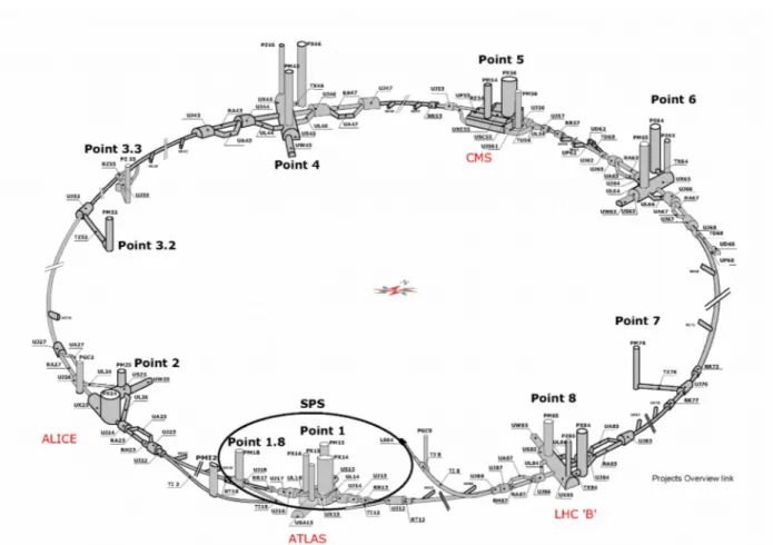
To reach the final design center-of-mass energy, the beams are accelerated through different stages performed using a chain of different accelerators (an overview of CERN accelerator layout is presented in Figure 2).

The different chain stages schematically described in Figure 3 LHC are:

• Linac2: It is a linear accelerator used as starting point for protons and ions. It

injects beams of 50 MeV in the following accelerator with a rate of 1 Hz. The

Figure 1: The underground structure of the LHC.

(11)

proton source is a bottle of hydrogen gas at one end of Linac2. The hydrogen passes through an electric field to strip off its electrons, leaving only protons to enter in the accelerator. The proton beams are pulsed from the hydrogen bottle impulses from 20 µs to 150 µs depending on the number of required protons. The pulses are repeated until enough protons are produced.

• Proton Synchrotron Booster (PSB): It speeds up the beams coming from Linac2

to an energy of 1.4 GeV. The accelerator is composed of four superimposed rings. In each ring, protons are collected in well defined packets or "bunches". They are them focused and sent through a magnet deflector into a single line to be injectied into the next accelerating element.

• Proton Synchrotron (PS): It is a key component in CERN accelerator complex.

It usually accelerates either protons delivered by the Proton Synchrotron Booster or heavy ions from the Low Energy Ion Ring (LEIR). The PS has a circumference of 628 metres and hosts 277 conventional electromagnets, including 100 dipoles, to bend the beams round the ring. PS accelerates protons up to an energy of 25 GeV. It has been set to separate the bunches by 25 ns, providing a bunch collision rate of 40 MHz.

• Super Proton Synchrotron (SPS): It is the second-largest machine in CERN

accelerator complex. Measuring nearly seven kilometres in circumference, it takes particles from the Proton Synchrotron and accelerates them to provide beams for the Large Hadron Collide. It has 1317 conventional electromagnets, including 744 dipoles to bend the beams round the ring. SPS is used as final injector for protons and heavy ions to LHC bringing the energy from 28 GeV to 450 GeV.

After the pre-acceleration stage the two beams are injected in the LHC ring at 450 GeV. Protons are them accelerated up to the design energy according the different periods of data taking.

(12)

LHC sheds light on an energy region almost unexplored yet. Most of the design parameters are therefore close to the technical limits.

The two beams circulate into two separate ultrahigh vacuum chambers at a pressure of 10-10 _{Torr. The beams are labelled 1 and 2, where the former circulates clockwise and the}

latter in the opposite direction.

To curve the beam trajectories and keep them inside the accelerator, 1232 superconducting dipole magnets are displaced along the track. Pictorial view of the

Figure 4: The key element of LHC accelerator: the 1232 dipoles bend the beam around the 27 km of circumference.

(13)

magnets is visible in Figure 4. They are based on the Nb-Ti superconductor, working at a current of 11.85 kA and a temperature of 1.9 K, maintained by a liquid-helium refrigerating system, generating a magnetic field of up to 8.4 T. Other 392 superconducting quadrupole magnets producing a field of 6.8 T are necessary to focalize the beams.

The most important parameters of LHC in 2015 data taking are reported in Table 1.

LHC parameters

Maximum collision energy 7 TeV Injection energy 450 GeV Dipole field 7 TeV 8.33 T Internal coil diameter 56 mm Peak luminosity 1034 _cm−2_s−1

Mean current 0.584 A

Bunch separation 24.95 ns, 7.5 m Number of particles per bunch 1.67 . ₁₀11

Crossing angle 300 µrad Life time of beam 10 h Energy lost per revolution (for proton) 7 keV Total power radiated by the beam 3.7 kW

Table 1: Main parameters of LHC during 2015 data taking.

Beam Structure

The two beams circulating in the accelerator are not continuous but they are structured in 3564 evenly spaced bunch slots, separated in time by 25 ns each. An identification number (ID) is assigned to every slot (filled or empty).When two bunch slots with the same ID are filled in the two different beams, they can collide at special interaction points along the LHC tunnel. This is referred to as a bunch crossing (BC) and every event can be associated with a Bunch Crossing ID (BCID) for timing purposes.

Depending on the operational status of LHC, different filling schemes are foreseen. At the designed luminosity each beam will contain 2808 filled bunches. The bunches will be

(14)

gathered in trains of 80, (72 filled and 8 empty), separated by 30 empty bunches. Each bunch will contain 1,15 x 1011 _{protons per bunch at the start of nominal fill and will be}

7.55 cm long. The same bunch structure is used for heavy ion data taking.

Assuming a total proton-proton cross section of 10-25 _cm-2 _{[3], there will be 10}9 _{events per}

second (or about 25 per BC). Elastic and anelastic collisions prevent the proton flows to circulate in the beam pipe in phase with the original bunches. A side effect of these collisions is that the beam luminosity degrades over time. The decay is exponential with an expected time constant t = 14.9 h, taking all loss mechanisms into account. Usually the beam can circulate for hours before a refill is needed. Measuring the luminosity is the task of various luminosity monitor detectors (see chapter 2).

1.1.2 LHC Experiments

Four experiments are installed along the LHC tunnel, see Figure 5 for a schematic view.

• A Toroidal LHC ApparatuS (ATLAS): it is a multi-purpose detector which

works at high luminosity. It has been designed to discover the Higgs boson as well as signatures of new phenomena in particle physics.

(15)

• Compact Muon Solenoid (CMS): it is another multi-purpose detector designed

to work at high luminosity with the same intents of ATLAS, but implemented with different and complementary technologies.

• LHCb: is the most specific experiment, it performs accurate measurements in the

flavour physics of the B-mesons, for example CP violation. Since the production and the decay vertices of B-mesons are difficult to reconstruct when there is more than one interaction per bunch crossing, LHCb works at a luminosity lower than the one designed for ATLAS and CMS, using proton beams less focused near the interaction point.

• A Large Ion Collider Experiment (ALICE): it is built mainly to study a

condensed status of the matter, called quark-gluon plasma, by detecting particles that are produced in heavy ion collisions. Due to the high nucleus-nucleus cross section, the higher track density per collision, ALICE can work up to luminosities L = 1027_cm-2_s-1_.

Other two experiments are installed along the tunnel:

• LHCf: it measures γ and Π spectra in the very forward region at luminosity of L =

1029_cm-2_s-1_{. The aim is the calibration of Monte Carlo generators in cosmic rays}

studies. This detector was installed in 2009 and worked during the data taking at 900 GeV. It will be reinstalled once the design center of mass energy will be reached.

• Total Cross Section, Elastic Scattering and Diffraction Dissociation at the LHC (TOTEM): it is designed to measure the total pp cross section at a

luminosity of L = 1029_cm-2_s-1_{. It is installed along the beam pipe near CMS.}

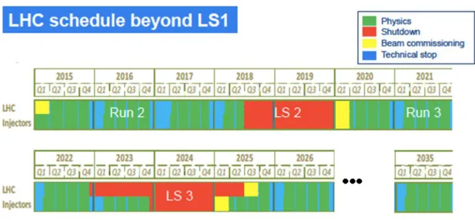
1.1.3 LHC Schedule

The Large Hadron Collider has started its second three-years run (RUN 2). Cool down of the vast machine has finished and LHC started again to run after a long technical stop weeded to prepare the machine for running with superior energy.

(16)

The accelerator chain, that supplies the LHC particle beams, was restarted. During the shut down period finished at the beginning of 2015, LHC and all the CERN accelerator complex had a major programme of maintenance and upgrading. Before to collide beams again, a long and careful testing has been done to check all functions of the machine. The aim of new data taking is to run the physics programme at 13 TeV in these years (from the beginning of 2015). The discovery of a Higgs boson is just the beginning of LHC journey. The increased energy opens the door to a whole new potential discovery, allowing further studies on the Higgs boson and potentially addressing unsolved mysteries such the dark matter.

(17)

1.2 The ATLAS Experiment

The ATLAS experiment is one of two general-purpose and a multi-purpose particle detectors, for physics studies, installed at the interaction point 1 of LHC, around 100 m underground. It probes a wide range of physics, from the search for the Higgs boson (discovery made public officially on 4 July 2012) to extra dimensions and dark matter particles. Although it has the same scientific goals as the CMS experiment, it uses different technical solutions and different magnet-system design.

The relative positions of the ATLAS experiment at Point 1 as well as its coordinates are shown in Figure 7.

The origin of the ATLAS coordinate system is defined as the nominal interaction point. The beam direction defines the z-axis and the x-y plane, transverse to the beam direction. The positive x-axis is defined as pointing from the interaction point to the center of the LHC ring. The positive y-axis is defined as pointing upwards. The A-side (C-side) of the detector is defined as the side with positive (negative) z. ATLAS is nominally forward-backward symmetric with respect to the interaction point [4].

ATLAS covers the full 2 π angle around the beam axis, in the polar ø coordinate, and an almost complete π coverage in the angle transverse to the beam axis.

Figure 7: Schema of underground facility where ATLAS is installed. The ATLAS coordinates are shown as well.

(18)

The detector is cylindrically symmetric, with a total length of 42 m and a diameter of 22 m [4]. With its 7000-tonnes, the ATLAS detector is the largest volume particle detector ever constructed. The detector is organized in a central barrel and two end-caps that close either ends. In the barrel, the active detector elements form cylindrical layers around the beam pipe while in the end-caps they are organized in wheel layers.

The cross sections of the most interesting new-physics phenomena are very small, if compared to the total cross section of the p-p interactions, for both the 8 TeV center of mass energy reached in the 2012 and the 13 TeV of 2015. A high luminosity is essential to produce copiously of these rare events and high precision detectors are necessary to measure the properties of particles produced at each interaction.

The ATLAS detector is composed by a large number of sub-detectors, and electronic components, that can be regrouped as:

• a Magnetic System composed of a central super-conducting magnet and three

toroidal magnets to bend the particle trajectories;

• an Inner Detector that provides the particle tracking close to the interaction point; • a Calorimeter System divided in electromagnetic and hadron calorimeter;

• a Muon System that tracks muons in the outer layers of the detector; • Luminosity Monitors that provide online luminosity;

• a Triggering System that selects bunch crossing containing interesting events and

stores only data with interesting physics signature;

• a System for data acquisition and distributed analysis.

1.2.1 The ATLAS Detector

The human eye is the most essential component of our visual perception ability and thus the main input for the analysis process that takes place in the human brain. It perceives light, photons, in a limited range of frequencies, making it fairly inapt at detecting fundamental particles in all possible energy ranges [5] [6] [7]. Detectors transform particles into visible inputs and to do this they exploit the different ways in which particles interact with matter.

(19)

ATLAS is composed of several subsystems, each designed for specific purposes.

Particles produced in collisions normally travel in straight lines, but in presence of a magnetic field their paths become curved. Electromagnets installed around the beam pipe generate magnetic fields to exploit this effect. Physicists can calculate the momentum of a particle – a clue to its identity – from the curvature of its path: particles with high momentum travel in almost straight lines, whereas those with very low momentum move forward in tight spirals inside the detector.

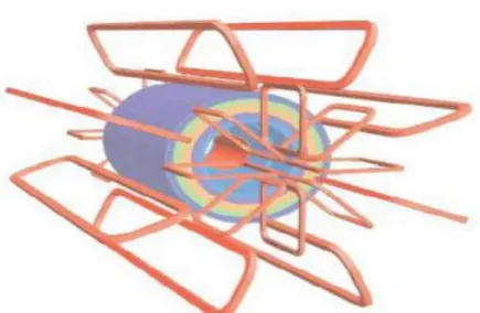
In Figure 9 scheme of the Barrel Toroids and of the End-Cap Toroid magnets (in red) installed in ATLAS are shown; the blue cylinder is the calorimeter.

(20)

The magnetic system of the ATLAS experiment is characterized by three different magnetic field systems, each of which is composed by superconductive magnets kept at a temperature of 4.8 K:

• Central Solenoid (CS): is designed to provide a 2T strong magnetic field in the

central tracking volume. It is a superconducting solenoid based on a thin-walled construction for minimum thickness to decrease particle scattering effects. In order to reduce material build-up and enhance particle transparency, the solenoid shares its cryostat with the liquid argon calorimeter (LAr). The superconducting solenoid installed around the Inner Detector cavity is 5.3 m long with a bore of 2.4 m, has a thickness of 45 millimeters, a weight of almost six tonnes and operates at a current of 7,600 A. The energy absorption of the solenoid is minimized through the use of a very thin coil and the sharing of the same vacuum vessel with the LAr calorimeter, in order not to alter significantly the performance of the calorimeters themselves. In Figure 10 a picture of the CS is shown.

Figure 9: Scheme of the Barrel Toroids and End-Cap Toroid magnets (red). The blue cylinder is the calorimeter.

(21)

• Barrel Toroid (BT): it consists of 8 rectangular coils arranged in cylindrical

configuration, super-conducting and air-core, with an open structure to minimize the multiple scattering effects. The total length is 25 m, with an inner diameter of 9.4 m and an outer diameter of 20.1 m. It is installed just outside the calorimeters. It provides a magnetic field of 1.5 T. In Figure 11 the BT of ATLAS is shown.

Figure 10: Scheme of the Central Solenoid (CS) in ATLAS.

(22)

• End-Cap Toroid (ECT): it is composed by 8 rectangular coils arranged in a

single cylindrical vessel. The total lenght is 5 m, with an outer diameter of 10.7 m and an inner one of 1.65 m. The vessel is mounted at the ends of ATLAS in order to close the magnetic field lines produced by the Barrel Toroid. With this configuration the magnetic field is orthogonal to the beam axis and has a value of 2 T.

Inner Detector (ID)

The Inner Detector (ID) is the inner part of ATLAS, near the beam pipe and closest to the interaction point. It contributes to particle identification and gives essential information to identify rapidly decaying particles. In Figure 12 a section of the ID is shown: it is constituted mainly of successive layers of subdetectors placed in a cylindical configuration around the beam pipe.

Approximately 1000 particles are expected to be produced every 25 ns for a luminosity of about L = 1034 _cm−2_s−1 _{within the ID volume [7], creating a very large track density in}

the detector.

(23)

The charge and direction of each track is measured, as well as the impact parameter, defined as the distance of closest approach to the beamline. The ID is also responsible for reconstructing both primary and secondary vertices, which are needed to identify B-mesons and converted photons. The ID is immersed in a 2T magnetic field. By measuring the curvature of the tracks, the momentum of the particles can be determined. The layout of the ID is presented in Figure 13.

Its structure is divided in three parts. A barrel section of ± 80 cm extending along the beam axis, closed at the extremities by two identical end-caps. In the barrel region high precision detector layers are arranged in concentrical cylinders around the beam axis while the end-cap detectors are mounted on disks perpendicular to the z-axis.

Given the very large track density expected at LHC the momentum and vertex resolution targets impose high-precision measurements to be achieved with fine-granularity detectors (usually semiconductor pixel).

The ATLAS Pixel Detector shown in Figure 14 provides a very high granularity, high precision set of measurements as close to the interaction point as possible. The system provides three precision measurements over the full acceptance, and mostly determines the impact parameter resolution and the ability of the Inner Detector to find short lived particles such as B-Hadrons. The system consists of three barrels at average radii of ~ 5 cm, 9 cm, and 12 cm (1456 modules), and three disks on each side, between radii of 9 and 15 cm (288 modules). Each module is 62.4 mm long and 21.4 mm wide, with 46080 pixel elements read out by 16 chips, each serving an array of 18 by 160 pixel. The 80 million pixel cover an area of 1.7 m2_{. The readout chips must withstand over 300 kGy of}

ionising radiation and over 5x1014_{neutrons per cm}2_{over ten years of operation. The}

modules are overlapped on the support structure to give hermetic coverage. The

(24)

thickness of each layer is expected to be about 2.5% of a radiation length at normal incidence. Typically three pixel layers are crossed by each track.

The pixel detector can be installed independently of the other components of the ID.

During the long shutdown between RUN 1 and RUN 2, an additional layer, called “b-layer” was inserted between the old Pixel Detector and the beam pipe.

In the intermediate radial range a SemiConductor Tracker (SCT) provides precise reconstruction of tracks as well as measurements of momentum, impact parameter and vertex positions, providing also good pattern recognition thanks to its high granularity. The barrel SCT shown in Figure 15 uses eight layers of silicon microstrips detectors to provide precision points in the coordinates. Each silicon detector is 6.36 × 6.60 cm2 _with

768 readout strips of 80 µm pitch. Each module consists of four single-sided p-on-n silicon detectors. On each side of the module, two detectors are wire-bounded together to form 12.8 cm long strips. The readout is accomplished by discriminator and a front-end amplifier, followed by a binary pipeline to store the hits above threshold, waiting for the Level 1 trigger decision (see section 1.2.3).

(25)

The end-cap modules are very similarly assembled, but they use tapered strips, with one set aligned radially. The detector contains 61 m2_{of silicon detectors, read out by 6.2}

million channels. Its high granularity is important for the pattern recognition.

The outermost component of the ID is the Transition Radiation Traker (TRT), is a combination of a straw detectors and a transition radiation detector, that can operate at the very high rates required by LHC. Electron identification is provided using xenon gas that becomes ionized when a charged particle passes through. This technique is intrinsically radiation hard and allows a large number of measurements, it is not as precise as those for the other two detectors, but it was necessary to reduce the cost of covering a larger volume and to have transition radiation detection capability.

Each straw is 4 mm in diameter for a maximum straw lenght of 144 cm in the barrel. The tubes are arranged in to 36 layers. A gold-plated tungsten wire in the middle of each tube collects the signal. Each layer is interspersed with a radiator to stimulate transition radiation from ultrarelativistic particles. The spatial resolution is about 200 µm.[4]

The barrel contains about 50000 straws, each divided in two at the center, with read-out at each end; the end-caps contain 320000 radial straws, with the read-out at the outer radius. The total number of electronic channels is 420000, providing drift-time measurements, with a spatial resolution of 170 µm per straw, and two independent thresholds, to discriminate between tracking hits and transition-radiation hits.

The Calorimetric System

Calorimeters in ATLAS are situated outside the solenoidal magnet that surrounds the Inner Detector. Their purpose is to measure the energy from particles by absorbing them. They detect also missing transverse energy by summing up all the measured energy deposits. A signal output in voltage or current proportional to the released energy is read out by front-end electronics and processed to recontruct the initial energy value.

(26)

The ATLAS calorimetric system is composed by two different calorimeters which cover different ranges of pseudo-rapidity. A pictorial view of the whole system is shown in Figure 16.

The Electromagnetic Calorimeter (EM Cal) is divided into a barrel part and two end-cap components. It is specifically designed to absorb and measure the energy from particles interacting electromagnetically, which include charged particles and photons. The EM calorimeter is composed by liquid argon as active material, with accordion-shaped kapton electrodes, and lead absorber plates as passive medium. When a particle traverses the liquid argon gap, it creates charge by ionization. Then the signal is collected on readout electrodes. The barrel component covers a region in pseudo-rapidity |η| < 1.475 while the two end-cap elements cover the range 1.375 < |η| < 3.2. The total thickness of the EM calorimeter is > 24 radiation lengths (X0) in the barrel and > 26 X0

in the end caps. The EM calorimeter must be able to identify electrons and photons with energy between 5 GeV and 5 TeV.

The energy measurements do not have to deviate from linearity more than 0.5% to provide good resolution [4].

The Hadronic Calorimeters are designed to absorb and measure energy from particles that pass through the EM calorimeter, but do interact via the strong force; these particles are primarily hadrons.

(27)

They are divided in different sections, the Hadronic Tile Calorimeter (HTC) is made of iron and plastic scintillator in the barrel region (|η| < 1.7), the second region is covered by a liquid argon calorimeter in the end-caps (Hadronic End-Caps Calorimeter, HEC) for 1.5 < |η| < 3.2 coverage, and two frontal Forward Calorimeters (FCAL), very close to the beam pipe, made of liquid argon, iron and tungsten, that covers the region of 3,2< |η| < 5. The thicknesses of the calorimeters have to be tuned in order to contain all the hadronic shower, to minimize the punch-through into the muon system and to provide a good resolution for high energy jets. The energy resolutions of the different sections have been measured in beam tests using pions and electrons.

Muon chambers

The muon spectrometer in ATLAS has been designed to be efficient in the muon detection and, in principle, should be able to measure the momentum without the help of the Inner Detector.

The muon chamber system, with its outer diameter of 22 m, represents the extreme outer layer of the ATLAS detector. The muon system is instrumented with separate trigger and high-precision tracking chambers for excellent momentum resolution.

The tracking chambers are Monitor Drift Tube (MDTs) chambers and Chatode Strip chambers (CSCs). The MDT chambers provide precise muon tracking over most of the pseudo-rapidity range. The tubes are made of aluminum and have a diameter of 30 mm. The resolution on the drift distance is about 80 µm [8]. The CSCs cover the pseudo-rapidity range of 1 < |η| < 2.7. They are multi-wire proportional chambers with cathodes segmented into strips. The spatial resolution on the coordinate is about 60 µm [8].

The trigger system covers the range |η| < 2.4. Resistive Plate Chambers (RPCs) are used in the barrel and Thin Gap Chambers (TGCs) in the end-caps. The trigger chambers (RPC and TGC) have a three-fold purpose:

• measurements of the second coordinate in the direction orthogonal to that

measured by the precision chambers, with a resolution 5-10 mm.

• bunch-crossing identification, separating events with a time resolution better than

25 ns;

• trigger with well defined pT threshold requiring a granularity of the order of 1 cm.

(28)

Only in a small fraction of pp collisions, high pT events can be found for standard model processes, and an even smaller fraction of events is expected to correspond to new physics. Muons at high pT or isolated ones are more common in interesting events than in background and provide thus an important signature used by the trigger system.

1.2.2 ATLAS Physics

LHC will give the chance to study a wide range of physical phenomena, to measure with high precision the parameters of Standard Model and to seek out details of the Higgs boson or new physics (e.g. supersymmetric events or dark matter).

To study the most fundamental laws of nature it is necessary to achieve very high energies [1] [9].

In the Standard Model, the mass is generated by the so-called Higgs mechanism, regulated by the interaction of each particle with Higgs field that provides at the same time the well-known Higgs boson.

The Higgs boson, elementary particle and massive scalar, was observed in the previous data taking period (RUN 1) but the Standard Model mechanisms have to be still understood. The Higgs boson has a fundamental role in the model: it explains why the

(29)

photon has no mass, while the W and Z bosons are very heavy. In electroweak theory, the Higgs generates the masses of the leptons (electron, muon, and tau) and quarks.

The predictions of the standard model agree very well with the results of all experiments performed so far, sometimes with a remarkable accuracy, but there are hints that it cannot be a complete theory. It is unclear if it can describe correctly the processes happening at very high energies and it does not explain some important features of our universe: most notably the matter-antimatter asymmetry and the dark matter/dark energy already observed in cosmological studies.

Supersymmetry is an extension of the Standard Model aimed to fill some gaps. Supersymmetry is the physical theory that correlates bosonic particles (that have integer spin) with the fermionic particles (which have half-integer spin). According to supersymmetry every fermion has a bosonic superpartner and every boson has a fermionic superpartner. These new particles would solve a major problem with the Standard Model – fixing the mass of the Higgs boson. If the theory is correct, supersymmetric particles should appear in collisions at the LHC.

Finally, in many theories scientists predict the lighest supersymmetric particle to be stable and electrically neutral and to interact weakly with the particles of the Standard Model. These are exactly the characteristics required for dark matter. The Standard Model alone does not provide an explanation for dark matter. Supersymmetry is a framework that builds upon the Standard Model strong foundation to create a more comprehensive picture of our world.

1.2.3 ATLAS Trigger and Data Acquisition System

ATLAS would produce about 1 Petabyte/second of raw data if all the pp collisions were recorded, at design luminosity. However, most of the data come from common, well-known processes that after the first studies, are not of interest for the experiment.. The purpose of a trigger system is to select just the rare, interesting events while rejecting everything else.

The ATLAS experiment relies on a complex and highly distributed Trigger and Data Acquisition (TDAQ) system to gather and select particle collision data at unprecedented energy and rates. The TDAQ is composed of three levels, which reduces the event rate from the design bunch-crossing rate of 40 MHz to an average event recording rate of about 200 Hz.

The acquisition system is the most composite subsystem present in the ATLAS experiment. Its issue includes all features associated with the transport of the physical data recorded by the various detectors in the experiment, the final storage of selected data, all devices needed to operate with the suitable custom electronics.

(30)

• electronics on the detector: so-called the "front-end electronics". Each detector

has a specific electronics, mainly analogic, that read out the raw data from the detector and send them to the next stage,

• transport electronics: the detector is placed 100 meters in the underground, in a

highly radioactive environment where there are strong magnetic fields; high flows of particles damage the performance of the more sensitive electronics. For these reasons the majority of the detectors have a custom board electronics to digitalize the signals directly for the cavern and to sent them far from the radioactive area;

• electronics data collection: the main task of these elements is to collect the raw

data, to digitize analog signals, to build data packets for each subdetector and to prepare them for the final phase of the acquisition. Such electronics are located in a protected environment at controlled temperature;

• electronics processing in situ: the data organized in packets and arranged for

sub-detector are subsequently selected through different levels of trigger and assembled to construct an ATLAS event. At this stage the data travel mainly over optic fiber and / or ethernet network-gigabit. Finally they leave the ATLAS experiment towards large calculus centers;

• off-site electronics processing: the first data collection center (called Tier) is at

CERN, the second in order of importance is in Bologna (Tier 1 of CNAF). These are large processing systems consisting of thousands of CPU server and organized in rack in which users can connect to perform the data analysis.

The Trigger System

The Trigger System [10] selects events containing interesting interactions among the huge amount of data produced at each interaction.

At the design luminosity there are about 25 interactions per bunch crossing leading to an interaction rate of about 109 _{Hz. The online triggering system must be able to select}

interesting physics signatures reducing the acquisition rate to approximately 200 Hz, the upper limit for the data storage. The goal is achieved with different trigger levels which successively refine the selection process: Level 1 Trigger (LVL1), Level 2 Trigger (LVL2) and Level 3 Trigger (LVL3) also called Event Filter. The differents levels of the trigger system is shown in Figure 18.

(31)

• Level 1 Trigger: all the subdetectors in ATLAS work at the full LHC

bunch-crossing rate. The trigger electronics has to provide a decision on the data temporarily buffered in pipe line at the rate of 40 MHz. The LVL1 trigger uses reduced granularity data from only a subset of detectors, muon chambers and calorimeters, plus prescaled contributions from luminosity monitors. Then the LVL1 decides if one event can be stored or it has to be rejected. The time to form and to distribute the trigger decision, called latency, is 2 µs and the maximum rate is limited to 100 kHz by the capabilities of the LVL2 trigger input band width. During the LVL1 processing, the data from all subdetectors are held in pipeline memories in the front-end electronics. The LVL1 trigger must identify unambiguously the bunch crossing containing the interaction of interest introducing negligible dead-time.

• Level 2 Trigger: the LVL2 trigger reduces the accepted rate from 100 kHz to 1

kHz, with a latency ranging from 1 ms to 10 ms depending on the event. Events passing the LVL1 trigger are held in so-called Read Out Buffers (ROBs) until the LVL2 trigger takes the decision to either discard the event or accept it. After an event is accepted, the full data are sent to the Event Filter processor via the Event Builder. In order to reduce the data transfer bandwidth from the ROBs to the LVL2 trigger processors, the LVL2 algorithms work on subsets of the detector data called Region of Interest (RoI) and defined in the LVL1.

(32)

• Event Filter the Event Filter trigger uses the full event data together with the

latest available calibration and alignment constants to make the final selection of events for permanent storage. At LVL3 a complete event reconstruction is possible, with a total latency of about 1 s. The Event Filter must achieve a data storage of 10-100 MB/s by reducing both the event rate and the event size.

LV2 trigger and Event Filter are called together High Level Trigger (HLT).

Data Acquisition System

The Data Acquisition System (DAQ) is the framework in which the Trigger System operates. It receives and buffers the data from the detector-specific read out, called Read Out Drivers (RODs), at the Level 1 trigger rate, and trasmits the data to the Level 2 trigger if requested. If an event fulfills the Level 2 selection criteria, the DAQ is responsible for building the event and moving it to the Event Filter. Finally, the DAQ forwards the final selected events to mass storage.

In addition to moving data down to the trigger selection chain, the DAQ provides an interface for configuration, control and monitoring of all the ATLAS detectors during data taking. Supervision of the detector hardware, such as gas system and power supply voltages, is handled by a separate framework called the Detector Control System (DCS). Moreover, the DCS is responsible for alert and handling archiving.

System of Synchronization

The syncronization of the LHC experiments to the collisions is necessary to guarantee the quality of recorded data. LHC provides beam related timing signals to the experiments via optical fibers that are several kilometers long. The phase of the clock signals can drift (e.g due to temperature fluctuation, causing front-end electronics to sample at non optimal working points). The syncronization at ATLAS is provided by the Beam Precision Monitor for Timing Purposes (BPTX) system [11]. The BPTX stations are composed by of electrostatic button pick-up detectors, located at 175 m from the IP along the beam pipe on both side of ATLAS. BPTX are used to monitor the phase between collisions and clock with high accuracy in order to guarantee a stable phase relationship for optimal signal sampling in the subdetectors front-end electronics. In principle, the bunch structure of the beams as well as the number of particles in each bunch can be measured by the BPTX system, but the accuracy on the number of particles is not high enough for a reliable luminosity measurement.

(33)

Measurements of Bunch Currents

Two complementary systems are used in ATLAS to evaluate the bunch currents with the precision required by luminosity measurements: the Fast Bunch-Current Transformers (FBCT) and the Direct-Current Current Transformers (DCCT).

The Fast Bunch-Current Transformers (FBCT) are AC-coupled, high-bandwidth devices which use gated electronics to perform continuous measurements of individual bunch charges for each beam. The Direct-Current Current Transformers (DCCT) measure the total circulating intensity in each of the two beams irrespective of their underlying time structure. The DCCT have intrinsically better accuracy, but require averaging over tens of seconds to achieve the needed precision.

The relative bunch-to-bunch currents are based on the FBCT measurements.

The absolute scale of the bunch intensities is determined by rescaling the total circulating charge measured by the FBCT to more accurate DCCT measurements.

(34)

Chapter 2 Luminosity Measurements

2.1 Introduction

The most important parameter when hadron-hadron collisions are studied is the energy available at the center of mass that can be transformed into particles. The LHC accelerator has been designed to reach a center-of-mass energy of 14 TeV (the highest world record) in order to have access to final states containing possibly the Higgs boson and other exotic particles. Since these processes are very rare and happen once every 109

interactions, it is important to produce as many events as possible at each collision. The machine parameter that is related to the yield of interaction is called instantaneous luminosity. The interaction rate is given by the product of the luminosity and the total inelastic cross section.

In any accelerator luminosity depends on several parameters, among which there are: number of particles circulating in the beam, the beam size in the plane transverse to the beam direction and the overlap of the two beams at the interaction point. For two perfectly head-on beams, the higher is the number of particles and the smaller is the beam size, the higher is the luminosity and hence the collision rate.

When the packets in the beam colide, the particles interact with eletromagnetic fields due to the presence of other protons. This process is well-known as beam-beam effect and it reduce the beam lifetime. During standard operation the packets remain inside the accelerator for about 10-20 hour. Beam-beam effect and interactions of protons with residual particles in the beam pipe degrade the number of particles in the packets, causing a continuous decrease of instantaneous luminosity.

The definitions of luminosity and its importance will be presented in section 2.2. The different methods used at LHC to measure the luminosity will be presented in section 2.3, with particular attention to ATLAS strategy.

(35)

2.2 Luminosity Overview

2.2.1 Istantaneous Luminosity

The instantaneous luminosity L in a collider is defined as the ratio between the total interaction rate R of any processand its cross section σ. It is expressed in cm-2_s-1 _{and it is}

independent of the process itself.

ℒ =_σR

The instantaneous luminosity can be inferred from the machine parameters: if the two beams are made of identical bunches, they are Gaussian in shape and overlap perfectly without crossing angle, the luminosity is given by:

ℒ =frnb

N₁N₂

4 Π σ_xσ_y

Detectors in ATLAS are generally able to determine only relative luminosity, mean an observable quantity related to the absolute luminosity through a calibration constant.

ℒ =μ_σnbfr inel = (μ vis ε )nbfr σinel = μvisn_bf_r ε σinel = μvisn_bf_r σvis where:

µ is the average number of interactions per bunch crossing (BC), σinel the inelastic cross section,

ε is the efficiency of the luminosity algorithm (including the acceptance) for a certain detector,

µvis_{= µ ε is the average number of interaction per BC as recorded by a particular}

luminosity monitor;

(36)

The absolute luminosity at LHC can be expressed in terms of colliding beam parameters in the transverse plane and, for zero crossing angle, it is given by the equation (1):

ℒ =n_bf_rI₁I₂

∫

ρ₁(x , y)ρ₂(x , y)dx dy (1) where:

I is the intensity of beam,

ρ1(x,y) ρ2(x,y) are the particle densities in the transverse plane of the beam 1 and 2

respectively,

dx, dy infinite elements of surface.

At LHC, due to beam losses of various origin, the instantaneous luminosity decreases by 1% every ten minutes according to the power law:

ℒ =ℒ₀e− tτ

where τ ≃ 14 h.

2.2.2 Integrated Luminosity

The integrated luminosity L is obtained by integrating the instantaneous luminosity over a certain time interval (t) and is expressed in cm-2_:

L=

_∫

0

t

ℒ (t ')dt '

The integrated luminosity L provided information on the total number of events collected in a certain period of time.

2.2.3 Delivered and Recorded Luminosities

The luminosity defined previously is called "machine luminosity" or the "delivered luminosity": it is the luminosity provided by the accelerator at a given interaction point. Since the physical analyses deal with recorded events, it is necessary to introduce another type of luminosity to take into account the data taking efficiency in order to keep

(37)

the proportionality between the events recorded and the physical cross section.

The recorded luminosity is defined summing up the delivered instantaneous luminosity for all periods of time when the apparatus was ready to take data. Obviously when the detector is switched off or not taking data the recorded luminosity is zero. During data taking there might be very short moments where the detector is not able to record data. These periods, called collectively dead-time, are usually originated by what happens just after a trigger is given or when the data taking system is momentarily busy. The recorded luminosity is therefore defined with respect to a trigger chain and refers to the fraction of time when the trigger chain was active. Bunch-crossing that occurs during dead-time are for example excluded.

The delivered luminosity is evaluated before any trigger decision and therefore does not test the dead-time of the data acquisition system. Since all datasets used for analysis are exposed to dead-time, the final goal is to find the recorded luminosity corresponding to the data-set in question: the delivered luminosity needs to be transformed into recorded luminosity by correcting for dead-time.

precise luminosity measurement are needed not only for offline physical analysis, but also online both for beam and data quality monitoring. Reliable real-time measurements of the instantaneous luminosity are a key ingredient for a successful data taking: these measurements provided to the LHC control room can be used to maximize the luminosity delivered at ATLAS.

2.2.4 Luminosity Monitor for Beam Tuning

In order to reach record luminosities, the LHC accelerator group has to accurately tune thousand of superconducting magnets making a single proton to circle billions of times before it collides with another proton. The accurate knowledge of the particle trajectories in the accelerator is ensured by several sensors along the accelerator and by what is recorded at the interaction points. To reach the optimal conditions for the highest delivered luminosity mini scans are used to center the beams on each other in the transverse plane at the beginning of each fill in LHC. Mini lumi-scans consist in active closed-orbit bumps around the IP, which modify the position of both beams by ±1σ in opposite directions, either horizontally or vertically. A closed orbit bump is a local distortion of the beam orbit that is implemented using pairs of steering dipoles located on either side of the affected region. In this particular case, these bumps are tuned to translate either beam parallel to itself at the IP, in either horizontal or vertical direction. The relative positions of the two beams are then adjusted, in each plane, to achieve the optimum transverse overlap, as inferred from the measurement of the interaction rate.

(38)

2.3 Luminosity Measurements in ATLAS

Luminosity measurements in ATLAS are designed to reach three goals.

• Providing final absolute integrated luminosity values for offline analyses, for the

full data sample as well as for selected periods. In addition, measurements of the average luminosity over small time intervals, called Luminosity Block (LB), and for individual bunch crossings are required. The LB is defined as a time interval in which the luminosity can be considered constant. As a consequence, the LB must be smaller than the decay time of the beam. The luminosity must be provided for each LB. In physics analyses, in fact, data are used only if some quality criteria, provided LB by LB, are satisfied. To avoid discarting too many data, short LB are needed. Typical values of LB lenght are thus of the order of 1-2 minutes, to balance all the aspects mentioned before. Each LB is identify by a number which uniquely tags it within a run.

• Providing fast online luminosity monitoring, as required for efficient beam

steering: machine optimization, as for example beam centering through miniscans, as well as efficient use of the trigger. The fraction of recorded data, called prescale, in fact, can be changed according to the beam degradation in order to optimize at each time the data acquisition band width. A statistical precision of about 5% per few seconds and systematic uncertainties below 20% are desirable for the online luminosity.

• Fast checking of running conditions such as monitoring the structure of the beam

and beam-related backgrounds.

Since there is no single experimental technique which can full fill all the above requirements, a number of complementary measurements and detectors have to be considered: parallel measurements of absolute and relative luminosity are mandatory.

2.3.1 ATLAS Running Conditions in RUN 2

During the RUN-1 period between 2009 and early 2013, the ATLAS trigger system [7] operated very successfully. It selected events with high efficiency at centre-of-mass energies up to 8 TeV, for a wide range of physics processes including minimum-bias physics and TeV-scale particle searches.

(39)

as summarised in Table 2 are expected to be challenging to the trigger system: trigger rates for a RUN-1-like system are expected to increase by a factor of roughly five in total.

A factor of two increase is expected from the increase of energy up to 13 TeV, and will be even higher for high pT jets. The additional factor of 2.5 originates from the

peak-luminosity increase from 8 × 10 33 _cm-2_s-1_{to 1-2 × 10}34 _cm-2_s-1_.

In addition, the peak number of interactions per bunch crossing (µpeak), which was 40

during the 2012 run, is expected to go up to 50.

The bunch spacing reduction from 50 ns to 25 ns, while helping to control the increase in in-time pile-up (interactions occurring in the same bunch-crossing as the collision of interest), will nevertheless increase both the out-of-time pile-up (interactions occurring in bunch-crossings just before and after the collision of interest) and beam-induced fake trigger rates, particularly in the muon system.

2.3.2 Relative Luminosity Measurements at ATLAS

As already mentioned, all ATLAS luminosity detectors can measure only a quality wich is proportional to the absolute luminosity, providing thus a “relative” luminosity measurements.

The luminosity monitors provide the measurements of the instantaneous luminosity at two different frequencies. First, the luminosity monitors evaluate the instantaneous luminosity at the frequency of about 1-2 Hz. These fast measurements are typically averaged over all bunch crossing in an LHC beam revolution (orbit). At least one of these measurements is communicated to the LHC for machine operations. Second, the instantaneous luminosity is provided LB per LB on bunch-by-bunch basis. These measurements are used for physics analysis.

In summary, the luminosity is provided both integrated over all the bunch crossings and on bunch-by-bunch basis.

The response of a luminosity monitor ought to be linear over a large dynamic range, fast,

Table 2: The luminosity acquired by the ATLAS experiment during RUN 1 and the expected RUN 2 luminosity.

(40)

stable in time and stable under different beam conditions. The main goal of these luminosity monitor detectors is to reach a stability better than 2%.

The detectors that can provide luminosity measurements (at different accuracy levels and pseudorapidities) during RUN 2 are:

• Beam Condition Monitor BCM: it covers |η| ~ 4.2 and provides precise

information on the condition of the beams and is thus used to calculate both integrated and bunch-by-bunch luminosity.

• Luminosity Cherenkov Integrating Detector LUCID: it covers 5.6 < |η| < 5.9 and

it was designed to sustain a high event rate and high radiation doses. It can work at design luminosity, and can provide both LB integrated and bunch-by-bunch measurements.;

• Hadronic Forward Calorimeters FCAL: is made of rod shaple electrodes inserted

inside a tungsten matrix. The FCAL provides electromagnetic as well as hadronic coverage in the very forward region 3.2 < |η|< 4.9. It can provide only LB integrated luminosity.

• Eletromagnetic End-Cap Calorimeter EMEC: consists of two wheels located on

either sides of the barrel. The outer wheel covers the region 1.375 < |η|< 2.5 while the inner wheel covers the region 2.5 < |η|< 3.2. It provides estimation of LB integrated luminosity.

• Tile Calorimeter TileCal: consist of alternating layers of plastic scintillator and

iron. It is a sampling hadronic calorimeter covering the pseudorapidity region -1.7 < |η|< 1.7. It provides LB integrated luminosity indirectly, monitoring the current drawn by the sensors.

In left plot of Figure 19, the integrated luminosities during stable-beam runs in 2011/2012 are shown: the LHC delivered luminosity is compared with the overall recorded luminosity at ATLAS and with the final luminosity recovered in perfect functioning conditions of the detectors (labelled "Good for Physics"). The losses of the delivered luminosity (for any reason) is around 10%.

In right plot of Figure 19 different evaluations of the instantaneous luminosity during a single run is shown for three of the luminosity monitors used in 2010 before any fine tuning correction. The decrease of the beam quality is clearly visible.

(41)

Relative luminosity must be calibrated through several methods, that exploit beam characteristics and known physics processes. The ﬁrst and most used calibration technique is performed using beam conditions in a van der Meer scan [12].

At the LHC the method consists in moving the beams transversely with respect to each others while recording the counting rate by all the available luminosity monitors. Separation scan are performed in both vertical and horizontal directions. The position of maximum rate is thus found and the absolute luminosity is inferred from the measured beam overlap. This kind of calibration has an uncertainty that depends on beam parameter uncertainty (beam current in particular) and on the extrapolation to the higher luminosity regimes; thanking to the improvement an that method during RUN 1 data taking, the final uncertainty of 1,9% has been reached in 2015 [13]. Calibration through physics channels, in particular the W and Z bosons, yields an uncertainty that depends on the limited knowledge of the parton distribution functions (PDF) [14], a value that has improved over the run and is now 3%, depending on the process used. Finally,∼ calibration through a dedicated detector (ALFA) [15] that measures the ﬂux of protons scattered elastically should lower the uncertainty down to 2%.∼

Figure 19: Integrated luminosity registered during runs in 2011/2012 and luminosity registered during the 2010 tests.

(42)

Chapter 3 The LUCID Detector

3.1 Introduction

The main topic of this thesis is to study the electronic system of the main luminosity monitor in ATLAS called LUCID (Luminosity measurements Using Cherenkov Integrating Detector).

The measurement of luminosity is essential in any high-energy physics experiment for cross-section evaluation. In ATLAS, luminosity is measured on several levels and at different steps of the data-taking and data re-processing:

•

online luminosity monitoring (performed by dedicated detectors), integrating signal over the short time-span Δt = 2s; only the fast hardware response of the electronics used by dedicated detectors can provide this measurement without significant delay;

•

lumi-block by lumi-block luminosity, integrated over a period of time in which the instantaneous luminosity is estimated to vary by less than 1%; this process allows Δt to vary between 30 s and 10 min, with an average value of 60 s;

•

offline luminosity, measured by reprocessing data in a more refined way; this measurement can be performed using a great number of detectors and algorithms, providing a redundant approach.

Since the start of data taking at the Large Hadron Collider, LUCID has been the only dedicated luminosity monitor in the ATLAS experiment [16] [12], although other detectors have been used to compute luminosity algorithms, as shown in chapter 2. The intrinsically fast response of the Cherenkov detectors and the dedicated readout electronics make it ideal to measure the number of interactions at each bunch crossing.

During the shutdown period between RUN 1 and RUN 2 (called long shutdown 1) a heavy upgrade of both detector and readout electronics have been necessary, to cope with

(43)

new LHC data taking conditions.

The solution to those problems was found by reducing the detector granularity and dimension. The reduced acceptance help LUCID to cape with the increased occupancy due to the higher center of mass energy and number of interaction per bunch crossing.

The original version of the detector (“old LUCID” [17]) is described in [ATLAS collaboration. JINST 3, S08003 (2008)] it took data providing luminosity values as main detector, in ATLAS during years 2009-2010 [18] and in combination with other detectors in years from 2011 to 2013.

In this chapter the “new LUCID” design will be presented with particular attention on the architecture of the sensors developed by the LUCID collaboration and especially on their read-out electronics based on Field Programmable Gate Array (FPGA).

3.2 Photo Multiplier Tubes

The Photo Multiplier Tubes (PMTs) are the sensitive part of the experiment and for this reason they take an important part in the R&D of the detector.

A photomultiplier is an instrument to measure and detect a light signal, in the visible or near ultraviolet range, converting it into electric current. Figure 20 shows the structure of PMT.

(44)

A PMT is constituted by a vacuum tube with an inlet window as much transparent as possible, a photocathode, a focussing electrode, a dynode chain in which a difference of potential is applied to collect and accelerate the electrons produced in the photocathode and an anode to collect current in output.

The operating principle of a photomultiplier is the photoelectric effect: the light incident on the photocathode produces electrons in quantity which is proportional to the incident light. The electrons are thus accelerated, by an the electric field, towards the first dynode, in which they are multiplied due to secondary emission. The procedure is repeated for a serie of dynodes and the final current is read out by the anode.

The most important components of PMT are thus:

• input window: since it is the first component encountered by incident photons, in

order to make photons detected, it has to be transparent with respect to the wavelength of the photons. According on the material used for the window, PMTs will have different lowest detectable wavelength. More over the chosen material has to be radiation hard if the PMTs have to operate in a strongly radioactive area as for example at LHC;

• photocathode is the plate on which the incident photons convert into electrons

(called photo-electrons) due to the photoelectric effect. The main parameter to be optimized is the energy estraction that has to be small in order to make easy the extraction of electrons by photons. The spectral response of the photocathode is the spectral response of the PMT and contains the information of the lowest and highest wavelength that photocathode can detect;

• dynodes: in order to produce a detectable signal even in case of very few incident

photons, the photoelectrons produced by the photocathode are accelerated through a chain of dynodes. At each stage the electrons are accelerated toward a dynode where, due to the acquired kinetic energy, they impinge and are able to extract 2-4 electrons that can be accelerated toward the next dynode. Several dynodes in sequence provide the multiplication chain needed to amplify the tiny signal of a single electron to a measurable electronic pulse. Normally a PMT uses 8 or 12 dynodes, arranged in a geometric configuration that permits to maximize the efficiency collection. The ratio between the number of electrons produced by the photocathode and the charge collected by the anode is called gain. The gain is related to the number of dynodes and to the voltage supply.

Two models of PMT have been used to replace the one installed in LUCID in RUN 1 (Hamamatsu R762), both of them with reduced window:

(45)

window of constant thickness of 1.2 mm, photocathode composed by bialcali.

• Hamamatsu R760 modified: as a previous one but modified by the constructors

with one part of the active window aluminized in order to further reduce the effective area to a diameter of 7 mm (shown in Figure 21).

3.3 Upgrade for RUN 2

The LUCID Detector worked in a strongly radioactive environment for a long time (more than three years). These working conditions caused ageing and performance degradation of LUCID. The main reasons of degradation are:

• Absorbed radiation: dosimeters, placed close to LUCID detector, measured a

radiation dose at LUCID position in agreement with expectations. The main source of radiation is gamma rays and, secondary, neutrons. A long exposure to radiation produced an internal radioactivity that caused an increase of the PMT anodic current even in absence of external light, called dark current. Its level was kept under control in order not to not invalidate the measurements.

• Current consumption: it is caused by the continuous hitting of the multiplied

electrons on the dynode metals. This degradates the dynodes by consumption (in particular the one closer to the anode, where the current impinging is higher). In

Figure 21: Image of the R760 PMT in its modiﬁed form, showing the circular aluminium layer that reduces the active area and, thus, the acceptance.