Analysis of the PC algorithm as a tool for the inference of gene regulatory networks: evaluation of the performance, modification and application to selected case studies

(1)

PhD Dissertation

International Doctorate School in Information and Communication Technologies

DISI - University of Trento

Analysis of the PC algorithm as a tool for the

inference of gene regulatory networks:

evaluation of the performance, modification and

application to selected case studies.

Emanuela Coller

Advisor: Co-advisor:

Prof. Enrico Blanzieri Dott. Claudio Moser

Università degli Studi di Trento Fondazione Edmund Mach

(2)

Il giorno piú bello? . . . Oggi. La cosa piú facile? . . . Sbagliarsi. L’ostacolo piú grande? . . . La paura. Lo sbaglio peggiore? . . . Arrendersi. La radice di tutti i mali? . . . L’ egoismo. La distrazione piú bella? . . . Il lavoro. La peggiore sconfitta? . . . Lo scoraggiamento. I migliori insegnanti?. . . I bambini. La prima necessitá?. . . Parlare con gli altri. La cosa che piú fa felici? . . . Essere di aiuto agli altri. Il Mistero piú grande? . . . La morte. Il peggiore difetto? . . . Il malumore. La persona piú pericolosa?. . . Il bugiardo. Il sentimento piú dannoso?. . . Il rancore. Il regalo piú bello? . . . Il perdono. La cosa di cui non se ne puó fare a meno? . . . La casa. La strada piú rapida? . . . Il cammino giusto. La sensazione piú gratificante? . . . La pace interiore. Il gesto piú efficace? . . . Il sorriso. Il migliore rimedio? . . . L’ ottimismo. La maggiore soddisfazione? . . . Il dovere compiuto. La forza piú potente del mondo? . . . La fede. Le persone piú necessarie? . . . I genitori. La cosa piú bella di tutte? . . . L’ AMORE! Maria Teresa di Calcutta

(3)

Abstract

The expansion of a Gene Regulatory Network (GRN) by finding additional causally-related genes, is of great importance for our knowledge of biological systems and therefore relevant for its biomedical and biotechnological applications.

Aim of the thesis work is the development and evaluation of a bioinformatic method for GRN expansion. The method, named PC-IM, is based on the PC algorithm that discovers causal relationships starting from purely observational data. PC-IM adopts an iterative approach that overcomes the limitations of previous applications of PC to GRN discovery. PC-IM takes in input the prior knowledge of a GRN (represented by nodes and re-lationships) and gene expression data. The output is a list of genes which expands the known GRN. Each gene in the list is ranked depending on the frequency it appears causally relevant, normalized to the number of times it was possible to find it. Since each frequency value is associated with precision and sensitivity values calculated using the prior knowl-edge of the GRN, the method provides in output those genes that are above the value of frequency that optimize precision and sensitivity (cut-off frequency).

In order to investigate the characteristics and the performances of PC-IM, in this thesis work several parameters have been evaluated such as the influence of the type and size of input gene expression data, of the number of iterations and of the type of GRN. A comparative analysis of PC-IM versus another recent expansion method (GENIES) has been also performed.

Finally, PC-IM has been applied to expand two real GRNs of the model plant Ara-bidopsis thaliana.

Keywords[bioinformatics, iterative method, PC algorithm, expansion, causal relation-ship, gene regulatory network, FOS-GRN]

(4)

(5)

List of Tables

3.1 Comparison of different LGN expansion algorithms. . . 44 4.1 Description of the DREAM4-Challenge 2 (time series) GRN. . . 47 4.2 Description of DREAM4-Challenge 2 (time series data of Escherichia coli ). 48 4.3 Description of DREAM4-Challenge 2 (time series data of Saccharomyces

cerevisiae). . . 48 4.4 Description of the 10 genes of the LGN, DREAM4-Challenge 2 and relative

interactions among these genes. . . 49 4.5 Description of the gene expression data from GEO database. . . 50 4.6 DREAM4-Challenge 2, Saccharomyces cerevisiae. . . 51 4.7 DREAM4-Challenge 2, Saccharomyces cerevisiae, rep3, size 10. In vivo

data (GEO). . . 52 4.8 Description of the gene expression experiments from PLEXdb used to test

the PC-IM. . . 56 4.9 Value of AUC and dmin with different tile size. . . 60

4.10 Values of AUC and dmin with different iteration number . . . 61

4.11 PC-IM performances with different gene expression data (SubSets A, B and C). . . 64 4.12 PC-IM performances in expanding FOS-GRN or a Random LGN. . . 65 4.13 Distribution of the expansion FOS-GRN genes into four classes. . . 66 4.14 Description of the three different LGNs used to compare the performances

of PC-IM and GENIES. . . 67 4.15 List of genes involved in the glycosilic pathway. . . 70 4.16 Description of SGD expression data. . . 74 4.17 Different combination of kernel matrix and algorithms to test GENIES. . . 75 5.1 Comparison of the LR+ value of PC-IM (314 PC-IM genes) and the LR+

value of Random Output genes (314 random genes). . . 79 5.2 314 expansion genes of FOS-GRN. . . 97

(8)

(9)

List of Figures

1.1 Example of a gene regulatory network. . . 2

1.2 General reverse engineering to infer GRNs. . . 3

2.1 Example of a directed graph G1. . . 13

2.2 Classification of different algorithms based on their specific domain of ap-plication. . . 15

2.3 Boolean model used to represent the relationship between input and output transcripts. . . 17

2.4 Representation and classification of the variables of a DAG G. . . 22

2.5 Different types of connections considered in the d-separation step. . . 24

2.6 Pseudocode of the PC algorithm. . . 25

2.7 PC algorithm schematic representation. . . 26

2.8 Schematic representation of the differences between the original PC algo-rithm and its modified versions. . . 27

2.9 Overview of the GENESYS algorithm. . . 30

2.10 Parameters generated by Growing algorithm. . . 32

2.11 Representation of the Gat-Viks and Ron Shamir methodology. . . 33

2.12 Schematic representation of the BN+1 expansion algorithm. . . 34

2.13 Overview of GENIES. . . 35

3.1 Schematic representation of PC-IM. . . 41

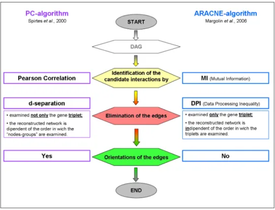
4.1 Scheme of the different strategies used by the PC and ARACNE algorithms. 53 4.2 Representation of the flower organs, ABC model and FOS-GRN of Ara-bidopsis thaliana. . . 55

4.3 Results of the preliminary evaluation 2. . . 58

4.4 ROC and PR curve of the tile size t effect. . . 61

4.5 ROC and PR curve of iteration number i effect. . . 62

4.6 ROC and PR curves for the dependence on different SubSets A, B and C. . 63

4.7 PPV-Se curve and ranking of the FOS-GRN expansion. . . 66 vii

(10)

4.10 ROC curve and PR curve of LGN 2. . . 71 4.11 ROC curve and PR curve of LGN 3. . . 72 5.1 Scheme of the phenylpropanoid biosynthetic pathway of Arabidopsis thaliana.

. . . 99 5.2 ROC curve and PR curve of the phenylpropanoid pathway. . . 100 5.3 PPV-Se curve and ranking curve of the flavonoids expansion. . . 101

(11)

Chapter 1

Introduction

The genome is the entire genetic material (DNA or RNA in many types of virus) of an organism (both unicellular and multicellular). It plays a central role in the control of all cellular processes (e.g. the response of a cell to environmental signals, the differentiation of cells and groups of cells in the unfolding of developmental programs, the replication of the DNA preceding cell division). The central dogma of molecular biology says that the genetic material (DNA) is transcribed into RNA (transcription process) and then trans-lated into protein (translation process). This is the basic mechanism of gene expression and it relies upon a unidirectional flow of the genetic information. Gene expression is finely regulated within the cell [Lewin and Dover, 1994] both at transcription and trans-lation levels and this control is essential to maintain cell homeostasis and to allow the organism life. Proteins may function as:

- transcription factors binding to regulatory sites of other genes; - enzymes catalyzing metabolic reactions;

- structural components of the cell;

- components of signal transduction pathways.

Different proteins may regulate the same gene or may form a single gene regulatory complex. Two genes can have a causal interaction without having a physical interaction. In fact there are indirect regulations via proteins and metabolism [Lauria and di Bernardo, 2010]. This variety of phenomena that regulates gene expression can be represented by Gene Regulatory Network (GRN).

GRNs are the complex systems that are formed from the regulatory interactions (causal relationships) between DNA, RNA and proteins. The final expression of a gene is deter-mined from these regulatory interactions between genes and proteins. In a biological cell

(12)

Figure 1.1: Example of a gene regulatory network.

Protein B and C independently activate gene D by binding to different regulatory sites on the promoter of gene D. Protein D represses gene C and interacts with protein A to activate gene B.

there are positive and negative regulations. In the positive regulation (or activation) the regulator activates the target genes, instead in the negative regulation (or inhibition) the regulator inhibits the target genes. Figure 1.1 reports an example of the gene regulatory network. More complex graphical conventions to represent cellular networks are proposed by Kohn [1999] and Kohn et al. [2006].

One of the objectives of molecular biology is to understand the regulatory mechanisms behind biological processes. This implies that a full description of a GRN determines the identification of the genes comprised in it, the comprehension of the gene connections (functional relations) and the elucidation of the kind of relationships between the genes of the GRN. A correct description of a GRN is of the greatest importance since it will allow either predicting the behavior of the system under perturbation or manipulating it for a specific aim [Bansal et al., 2007]. The problem is that the knowledge of biological systems is incomplete, therefore the construction of putative biological models and GRNs are necessarily based on incomplete information.

An approach to this problem is to adopt the principles of reverse engineering. Reverse engineering is the process that, starting from iterative experimentation (for example gene expression data) on an unknown system, arrives to the reconstruction of GRNs. Figure 1.2 is a schematic drawing of the process of reverse engineering. The strategy starts from

(13)

3

Figure 1.2: General reverse engineering to infer GRNs. (taken from [Gardner and Faith, 2005]).

experiments of cell perturbation with various treatments. In the second step, the aim is to measure the expression of the transcripts. Subsequently, a learning algorithm infers the model of transcription regulation using the expression data. The final result is the gene regulatory network.

This approach requires large data sets and extensive computational resources, because there is a big number of network architectures that are compatible with the same ex-periment results (set of expression data) [Tegner et al., 2003]. Luckily, in recent times the quantity of information that is available for reverse engineering is enormous. In fact, the genome projects have rapidly generated large datasets of sequences of genes and pro-teins that govern cellular behavior. Moreover 20 years ago [Schena et al., 1996] [Chee et al., 1996] [Lockhart et al., 1996] gene expression microarrays permitting of simultane-ously measure thousands of transcripts [Schwarz, 1978]. The array technology has several limitations [Marioni et al., 2008]:

- background levels of hybridization limit the accuracy of expression measurements, particularly for transcripts present in low abundance;

- probes differ considerably in their hybridization properties and this affects the com-parison of hybridization results across arrays;

- arrays are limited to measure abundance of transcripts with relevant probes on the array;

- arrays do not allow to measure DNA methylation and other DNA modifications. Sequencing-based approaches to measure gene expression levels have the potential to overcome these limitations (454 Life Sciences -Roche- [Margulies et al., 2005], Illumina-Solexa sequencing- [Bennett et al., 2005]). Despite this, microarrays are still widely used,

(14)

because the new technologies are complex and data available on public sites are still limited both in quantity and in number of different organisms analysed.

1.1 Objective of the Thesis

The aim of this thesis work is the development of a method to expand a characterized Gene Regulatory Network, called Local Gene Network (LGN) in the following. The expansion leads to the identification of new genes that are related with the known genes of the LGN. These are listed in a final expansion gene list which reports as well an estimate of their reliability. The expansion genes are obtained analyzing all the genes of interest given in the input list together with the corresponding gene expression data loaded by the user. Before expanding a LGN, the whole input gene list is subdivided in subgroups (called tiles). Each tile contains different genes of the input gene set, but all include the genes of the LGN. The whole expansion procedure is iterated i times and the final output takes into account the output of all the iterations. Subsequently, the reliability is determined by an intrinsic performance evaluation. This step requires to calculate precision and sensitivity within the genes of the LGN and then to project these values on the new genes. The procedure is called PC-Iterative Method (PC-IM). The term PC indicates that our algorithm uses the causal discovery algorithm developed by Spirtes and Glymour (PC algorithm) [Spirtes and Glymour, 1991], instead the "iterative"term indicates that the analysis of the whole input gene-set is repeated more times. Though our method was designed to use the PC algorithm, this does not exclude that the algorithm may change. In fact the user can substitute the PC algorithm with the algorithm that he prefers.

Novel aspects

The innovative contribution of this thesis is mainly related to the LGNs expansion task as mentioned above. In particular it is innovative how the task is treated (use of the LGN knowledge, type of gene expression data) and the type of obtained output.

• Task and method

The LGN expansion idea originates from two considerations. The first is that, often, a biological researcher has prior knowledge about relevant genes and their involvement in a LGN and he is willing to expand this knowledge. The expansion is obtained, at the beginning, with hypotheses formulation about other putative interactions of these genes with new genes and subsequently with the in vivo validation of this hypothesis by new experiments. The hypotheses can be formulated with bioinformatic systems (use of al-gorithms to infer regulatory networks, in silico coexpression analysis of gene expression data). The second consideration is that quite often the LGNs proposed by the commonly

(15)

Objective of the Thesis 5

used algorithms are complex, and thus it is difficult for a researcher to design the appro-priate biological experiment to validate the results. In fact in vivo validation requires the characterization of all the genes of the new gene network. The techniques commonly used to measure gene expression on a large scale (such as microarray experiments) can not be used, because, often, they are the input of the algorithm. Other useful techniques to vali-date the in silico results are, for example, the chip-seq tecnique, which studies the binding sites of the transcription factor or the manipulation of a specific gene in the homologous or heterologous system (knock-out or over expression). In general these approaches can be used only to test few genes, because they require long times and they are labor intensive and costly.

In literature, a big number of articles try to infer new gene networks by identifying new causal relationships among genes [Penfold and Wild, 2011]. These articles describe algorithms, as were described in Chapter 2, or website platforms (also called web-based tools) which are big collections of different types of data (publications, information about gene annotation, gene expression and chemical data) used to reverse engineering putative gene-gene interactions. There are two principal classes of website platforms. The first class comprises the web-based tools that use prior knowledge about a GRN as scaffold and then use gene expression data to validate the relationships between genes (e.g. BAR [Toufighi et al., 2005], BioGRID [Stark et al., 2006], GeneMANIA [Mostafavi et al., 2008]). It is important to underline that the GRN scaffold derives from the published information and it may not contain all the gene-gene interactions because it may not represent the only true biological network that involves the studied genes. In fact, it is possible to miss gene-gene interactions that can be associated with specific phenotypes or specific development conditions, which are not present in any publication. It is also possible that the same genes are involved in more GRNs. The second class, instead, is represented by web platforms that use a combination of information deriving from public databases and gene expression data to infer GRNs (Predictive Networks [Haibe-Kains et al., 2012], bioPIXIE [Myers et al., 2005]).

The task of GRN expansion is recent and therefore few publications are available up to now. This fact highlights the importance and novelty of this topic. One of the first algo-rithms developed for GRN expansion was GENESYS [Tanay et al., 2001]. Subsequently other methods were proposed; namely Growing algorithm [Hashimoto et al., 2004], Gat-Viks and Ron Shamir [Gat-Gat-Viks and Shamir, 2007], BN+1 [Hodges et al., 2010], ANAP [Wang et al., 2012] and GENEIES [Kotera et al., 2012]. All these systems have in common with our method PC-IM the task, but differ in the approach used for the expansion.

GENESYS (GEnetic Network Expansion SYStem) [Tanay et al., 2001] is an algo-rithm that uses gene expression data to expand a known LGN. It proceeds with three

(16)

steps:

1. Standardization of the data of the input dataset;

2. Use of a priori information about LGN to obtain the fitness function. The fitness function is the criterion wich guides the selection of the expansion genes;

3. Expansion of the LGN analyzing a gene at a time and using the fitness function as selection criterion.

Growing algorithm [Hashimoto et al., 2004] uses the gene expression data to expand little LGNs (one or more genes) and prior knowledge about these LGNs is not mandatory. This method can be divided in two steps:

1. Measure of three parameters which reflect the strength of the connection between two genes. These parameters are measured between genes of the LGN, between the genes external to the LGN and between genes of the LGN and genes outside the LGN;

2. Combination of these three parameters in an unique criterion subsequently used to expand the LGN.

Gat-Viks and Ron Shamir [Gat-Viks and Shamir, 2007] in the 2007 have developed a system that uses gene expression data and prior knowledge to expand LGNs [Gat-Viks and Shamir, 2007]. Gene expression data must derive from experimental procedures (gene silencing or enhancement of the gene expression). There are three steps:

1. Modeling the prior knowledge. This implies that an evaluation model is created using a priori information about LGN, Bayesian scoring matrix and probabilistic modeling;

2. Generation of the predicted evaluation model from the experimental gene expression data;

3. Comparison of the predicted and observed evaluation model to discover the expan-sion genes of the LGN.

BN+1 [Hodges et al., 2010] is a system that uses the gene expression data and prior knowledge to expand a LGN. The steps are the following:

1. Generation of multiple cores Bayesian Networks (core BN) using gene expression data, prior knowledge of the LGN and the log posterior score;

(17)

2. Selection of the core BN with the highest log posterior score [Heckerman et al., 1995]. This core BN will be the LGN to expand;

3. Expansion of the core BN adding a gene at a time. The final expansion gene list will contain only those genes that improve the score determined in the second step. GENIES [Kotera et al., 2012] discovers the new genes related with a specific LGN using a kernel function [Kotera et al., 2012]. It uses a priori information about LGN and different type of data in combination or alone (gene expression data, protein localization data, phylogenetic profile, kernel matrix based on the gene expression profile, kernel ma-trix based on the protein localization profile and kernel mama-trix based on the phylogenetic profile). It works in three steps:

1. Transformation of each data set in a kernel similarity matrix;

2. Mapping of the knowledge about LGN in a feature space (training process) equipeed with the Euclidean distance [Yamanishi et al., 2005].

ANAP [Wang et al., 2012] is a tool that was developed only for Arabidopsis thaliana. It integrates 11 Arabidopsis protein interaction databases, 100 interaction detection meth-ods, 73 species that interact with Arabidopsis and 6.161 references [Wang et al., 2012]. This tool may expand the network only using the interaction detection methods present in its database, instead PC-IM and other methods listed above use the data loaded by the user (gene expression or other type of data).

• Usage of the LGN prior knowledge

Another innovative aspect of PC-IM is the step in which the prior knowledge of the LGN is used. All methods mentioned above use the prior knowledge at the beginning of the expansion process. Instead PC-IM uses a priori information in two different moments. At the beginning it uses, as prior knowledge, only the names (genes identifications) of LGN’s genes to add them to the tiles. These genes will be the only genes present in all the subdivision of the input gene-list, instead the other genes will be present only in a single tile. Subsequently, the LGN knowledge will be used, at the end, to estimate the precision of the genes in the output expansion gene list. Practically, the genes of the LGN are treated as any other gene when applying PC-IM, while in the other expansion methods (GENESYS, Growing algorithm, Gat-Viks and Ron Shamir algorithm, BN+1, ANAP and GENIES), the prior knowledge of the LGN is used to construct a scoring matrix to be improved with the addition of the expansion genes.

(18)

PC-IM differs from the algorithms cited above also for the criterion used to select the final expansion gene list.

PC-IM uses the normalized frequency to determine which genes will be included in the expansion gene list of a LGN. The frequency corresponds to the number of times that a gene is found to expand a LGN with respect to the times that the same gene could be found. Each gene, not included in the LGN, can be present just once for iteration, namely it is present in only one tile. The frequency calculated on the LGN genes is used as a cut-off frequency to select the other genes.

GENESYS uses the fitness value. This is a numerical value that expresses the perfor-mance of an individual against other different individuals. In case of the expansion task the individuals that are presumed to have higher fitness values are the genes in the LGN, while the other individuals are the external genes [Liang et al., 1998]. Growing algo-rithm uses the strength of a connection to expand a LGN. This strength is determined from the coefficient of determination [Hashimoto et al., 2004].

"The coefficient of determination gives an indication of the degree to which a set of variables improves the prediction of a target variable relative to the best prediction in the absence of any conditioning observations "[Hashimoto et al., 2004].

Gat-Viks and Ron Shamir algorithm uses the Bayesian score [Gat-Viks and Shamir, 2007]. It is used as selection criterion of the model predictions to the data.

BN+1 uses the log of the BDe. This is the natural log posterior and its specific formulation is in Hodges et al. [2010].

GENIES uses the Euclidean distance to obtain the expansion genes. The Euclidean distance is calculated between genes of the LGN and between the hypothetical expansion gene and LGN genes. The Euclidean distance between the LGN genes is the threshold to select other genes [Kotera et al., 2012].

• Gene expression data: observational data

In PC-IM, the inference of the GRN is based on a particular type of gene expression data called observational data. This type of gene expression data is present in public databases, but it is rarely used for inference of networks. In fact there are two different strategies to determine GRNs from gene expression data. One relies on data measured in a perturbed biological system (experimental perturbed data) [Davidson et al., 2002], the other on the natural variation of expression levels of the same gene in different cells (observational data) [Chu et al., 2003] [Yoo et al., 2002].

The experimental approach is based on the suppression or the enhancement of the expression of one or more genes using transgenesis or natural mutants, and the measure-ment of how the gene expression is influenced [Davidson et al., 2002]. With this method

(19)

is relatively easy to identify the genes involved in the GRN and it has proved fruitful in unraveling small parts of a regulatory network. However, this approach has some disad-vantages. It provides information only about the effects of one or few manipulated genes and its gene targets. Moreover, in complex organisms, such as human and plants, this type of data is difficult to obtain due to the long time to collect them and to ethical issues. The second approach relies on observational data, and it overcomes these problems. In fact it permits to determine multiple relationships without any experimental inter-vention. The observational data are obtained merely observing a phenomenon (natural variation of the expression level) when the organism is in the natural (or optimal) de-velopment condition and when is under stress condition (water stress, cold stress, salt stress). In this case the GRN is inferred from statistical dependencies and independences among the measured expression level [Chu et al., 2003] [Yoo et al., 2002]. Despite the abundance of observational data present in the public databases only few algorithms use them [Spirtes et al., 2001] [Pearl, 2002] [Emmert-Streib et al., 2012], since they require elaborate statistical procedures.

The development of a system able to infer gene networks starting from observational data is of great importance since it allows to exploit the big availability of the data stored in public databases. This is an innovative aspect of this work. Moreover, this is also important because it allows to use public data and to find new genes involved in a specific LGN in a early stage of the biological investigation. This possibility offers the advantage of using new information to specifically design the experiment for novel genes validation.

• Final output

An innovative contribution of this thesis is the formulation of an alternative strategy to expand a Local Gene Network (LGN) by identifying only the additional genes that are related with at least one LGN-gene. In other terms PC-IM returns an expansion gene list, without specifying which genes of the LGN have a direct relationship with the genes in the expansion gene list.

In the expansion process of a LGN, as the inference of a GRN, there are two important steps. The first step regards the identification of the genes that expand the LGN. The second regards the identification of the causal relationships between the new genes and the LGN genes. Causal relationships are defined by the connection between two genes (relationship) and the orientation of this connection (causal direction). If y and x are two genes, and in particular y is affected by x (the presumed cause), there are three conditions that determine the exact causality (direction of the relationship) between these two genes [Kenny, 1979]:

(20)

2. x must be reliably correlated with y (beyond chance);

3. the relation between x and y must not be explained by other causes.

Nevertheless these three conditions are necessary, but not sufficient to find all possible causal relationships. This because there are cases (reciprocal causation and simultaneous causation) that are not explained by these conditions [Antonakis et al., 2010].

Reciprocal causation: in gene networks, there is a possibility that two variables are reciprocally cause and effect. This occurs when the expression of gene x activates gene y and the encoded protein inhibits the expression of gene x. A biological example is the lac operon [Van Hoek and Hogeweg, 2007]. In the lac operon an increased concentration of lactose in the cell causes an increase of the lac operon activity. Simultaneously an increase of the activity of this operon decreases the lactose cellular quantity.

Simultaneous causation is the activation of a target gene by the action of more genes together. For example this happens in tryptophan synthesis. In this case a trypthophan operon controls the synthesis of the enzymes that produce tryptophan. The operon is regulated by a repressor that alone is inactive, but is induced when it combines with a specific molecule [Hamon et al., 1981].

These two considerations show that it is very difficult to find by in silico analysis the exact causal relationship between two genes. It is easier to identify the list of genes that expands a LGN. Moreover this information (the list of genes) is enough to design in vivo validation experiments. The experiments will help in validating the new genes and to discover the causal relationships between the genes and the LGN genes. For the above reasons we choose the expansion task, (focusing on the list of the expansion genes and not on the causal relationship), rather than discovery of new GRNs.

1.2 Structure of the Thesis

The thesis is composed of four main Chapters. Chapter 2 presents an overview of the different types of reverse engineering algorithms in Section 2.1 and a detailed description of the PC algorithm and its related applications in Section 2.2. Section 2.3 a description of the methods used to expand LGN is reported. The other three Chapters describe the results of my PhD work. Chapter 3 reports the description of PC-Iterative Method (PC-IM). Chapter 4 presents the Evaluation of PC-IM. It starts with a section dedicated to a preliminary evaluation in which the expression data for testing the performance of the method are selected (Section 4.1) and the choice of the PC algorithm is motivated (Section 4.2). Afterwards in Section 4.3 an evaluation of the PC-IM is presented. This includes the assessment in terms of the performance of the single parts of our method.

(21)

Structure of the Thesis 11

Finally Chapter 5 is focused on the real expansion of a specific Local Gene Network with PC-IM and two case studies are described.

(22)

(23)

Chapter 2

State of the art

Causation is a relationship between an event (the cause) and another event (the effect). The second event (the effect) is interpreted as a consequence of the first event and it can have more than one cause [Spirtes et al., 2001]. Causation has three properties; it is transitive, irreflexive and antisymmetric.

- if X is a cause of Y and Y is a cause of Z, then X is also a cause of Z (transitive property);

- an event X cannot cause itself (irreflexive property);

- if X is a cause of Y then Y is not a cause of X (antisymmetric property).

Causal inference is the process used to obtain conclusions about presence/absence of causal relationships between events. To draw to these conclusions statistic means are used [Spirtes et al., 2001]. To represent causality we can use a directed graph. A directed graph consists of a set of vertices (e.g. genes) and a set of directed edges (e.g. relationship between genes), where each edge is an ordered pair of vertices. In Figure 2.1 an example of a directed graph G1 is depicted and below we report the terminology associated to the graph.

- the vertices are {A, B, C, D, E};

(24)

- the edges are {B → A, B → C, D → C, C → E};

- B is parent of A, because there is an oriented edge from B to A; - A is child of B;

- A and B are adjacent, because there is an edge between the two variables; - a path is a sequence of adjacent edges (A ← B → C);

- a directed path is a sequence of adjacent edges all pointing in the same direction (B → C → E);

- C is collider on the path because both edges on the path are directed into C; - E is descendent of B (and B is an ancestor of E), because there is a directed path

from B and E. Each node is ancestor and descendent of itself.

When a directed graph does not have cycles, then it is called directed acyclic graph (DAG). This means that in the DAG there is no directed path from any vertex to itself.

The causality representation by directed graph and/or DAG presents some problems. For example in the graph G1 considering A → C ← B we are not able to represent the situation in which there are two different drugs (A and B) that reduce symptom C, and A can reduce the symptom C also without B, instead B alone has no effect on C. Moreover we are not able to represent the situation in which there are two independent variables A and B with two states. For example A is a battery and the two states are charged and uncharged; B is a switch and two states are on, off. A and B cause C (A → C ← B), only when A and B are simultaneously verified (A indicates the battery charged and B the switch on) [Spirtes et al., 2001]. These problems arise, because the relationships are represented through the probability distribution associated with the graph [Spirtes et al., 2001].

As mentioned in Chapter 1, the use of the transcript levels to identify regulatory influences between genes is called reverse engineering (or inverse modeling or network inference). There are two classes of reverse-engineering algorithms: those that search for physical interactions and those which search for influence interactions [Gardner and Faith, 2005]. The aim of the physical interaction’s methods is to identify the binding motifs of transcription factors and identify thus their target genes (gene-to-sequence interaction). Influence interaction methods, instead, seek to relate the expression of a gene to the expression of the other genes in the cell (gene-to-gene interaction). In this work the ensemble of these influence interactions constitute a gene network. In this section we present a brief review of the principal algorithms developed to find influence interactions. Obtaining a gene network from influence interactions is useful for multiple purposes:

(25)

Gene network inference algorithms: a review 15

Figure 2.2: Classification of different algorithms based on their specific domain of application (adapted from Lauria and di Bernardo [2010])

1. identification of the genes that regulate each other with multiple (direct and/or indirect) interactions;

2. prediction of the response of a network to perturbations;

3. identification of the real physical interactions. This identification is obtained by the integration of the gene network with additional information from sequence data and other experimental data (i.e. chromatin immuno-precipitation [Das et al., 2004] or yeast two-hybrid assay [Bartel and Fields, 1997])

2.1 Gene network inference algorithms: a review

PC-IM was developed with the PC algorithm, but theoretically it can be used also with other algorithms. For this reason in this section a review of the main algorithms used to infer gene networks is included.

Figure 2.2 shows the different domains of application of the most used algorithms according to the type of experiments that have generated the input data.

(26)

In the algorithm’s description we will use the following variables: i are the genes;

N is the total number of genes;

xi is the expression measurement of gene i ;

X is the set of expression measurements for all the genes;

M is the total number of time points (or different conditions) of the expression mea-surements;

aij is the interaction between gene i and j.

In the undirected graph, the direction is not specified and aij = aji, instead when aij 6= aji

we have a directed graph. A directed graph can also be labeled with a sign and strength for each interaction aij > 0 means that there is activation, instead aij = 0 means there

is no interaction and aij < 0 indicates the repression). The choice of the type of graph

(directed or undirected) depends on the inference algorithm. 2.1.1 Clustering algorithms

Clustering algorithms divide the genes in groups (clusters). In each group there are genes with similar expression profiles (coexpressed genes). The coexpression between genes does not imply, however, the direct interaction among these genes [Lee et al., 2004]. In fact genes that are coexpressed can be related together by one or more intermediaries (indirect relationships). For this reason the clustering algorithms are not properly network inference algorithms, but are rather used to visualise and analyse gene expression data. Moreover the coexpression analysis can be used to deduce the function of genes from other genes in the same cluster [Eisen et al., 1998].

The most common clustering algorithm is the hierarchical clustering [Eisen et al., 1998]. It searches to obtain a single tree where the branch lengths reflect the degree of similarity between the genes. The connection between genes is assessed by a pairwise similarity function (for example Pearson correlation). The highest value of the pairwise correlation coefficient indicates that there is a relationship between the pair of genes [Eisen et al., 1998].

Another algorithm is the signature algorithm [Ihmels et al., 2002]. It is specialized to identify transcription modules starting from gene expression data. The transcription module is a group of genes that are co-regulated in particular experimental conditions. This algorithm enables gene classification, namely a clusterization of genes into different groups [Ihmels et al., 2002].

(27)

Figure 2.3: Boolean model used to represent the relationship between input and output transcripts (taken from Gardner and Faith [2005]).

2.1.2 Network Inference Algorithms

The inference of GRNs from expression data is a difficult task, mainly because the number of variables is much larger than the number of observations. Following a description of the most common algorithms developed to this aim.

Boolean network models

Kauffman proposed the first Boolean model [Kauffman, 1969]. They represent genetic networks as interconnected binary elements, with each of them connected to a series of others [Kauffman, 1969]. In the GRN the binary elements are the genes and each element can have two binary states, inactive (0) or active (1) and the interaction between the elements are modeled as Boolean rules. This mean that, if fully connected, a Boolean network with N genes will present 2N _{gene expression patterns. This number is very}

high and requires large amount of experimental data [Gardner and Faith, 2005]. For this reason, it is assumed that networks are sparsely connected and this shows the importance to specify the connectivity. Moreover the Boolean network can be represented as a directed graph, where the edges are represented by Boolean functions (simple Boolean operations, e.g. AND, OR, NOT). In general a repressor is equivalent to a NOT function, whereas cooperatively acting activators are represented with the AND function. In this way, the Boolean variables (where the states of genes can be 1 or 0) are determined at time t+1 by the state of the network at time t, the value of the K inputs and the logical function assigned to each gene. Figure 2.3 is an example of Boolean model in which the OR logic function is illustrated. In this representation there are three transcripts X1, X2 and X3

and K has value 2. This implies that the possible networks, with the three variables, are 4.

The final aim of the Boolean method is to identify a Boolean function for each gene in the network that it explains the model. This class of algorithms have been used to describe different biological pathway, including signalling pathway [Shymko et al., 1997]

(28)

[Genoud et al., 2001] and bacterial degradation processes [Serra and Villani, 1997]. In the literature various Boolean algorithms have been proposed. One of this is REVEAL (REVerse Engineering ALgorithm; [Liang et al., 1998]). "REVEAL was developed to allow for multiple discrete states as well as to let the current state depend not only on the prior state but also on a window of previous states"[Hecker et al., 2009].

Bayesian network models

Bayesian Network (BN) models are graphical representations of joint probabilistic distri-butions of a set of random variables Xi (i.e. gene, protein or other cellular elements).

A BN has two components [Pe’er, 2005], the first component is a DAG that represents the relationships between the variables. Its vertices are the random variables Xi and the

edges represent the influence of one variable on another. The second component, denoted with θ describes a conditional probability distribution for each variable Xi.

The principal limitation of the BN is the absence of cycles in the network as well as the explicit treatment of causality among the variables. The absence of cycles derive from the use of the DAG to represent the network. This is a problem, because the cycle systems are relevant in biological systems (for example the feedback loops among the B-C variables in Figure 1.1). The other issue is that BNs represent the probabilistic dependencies among variables and not causality. This mean that the parents of a node are not necessarily also the direct causes of its behaviour, in our case its gene expression [Bansal et al., 2006]. To overcome these limitations the Dynamic Bayesian Network (DBN) was developed [Yu et al., 2004]. DBNs can establish the direction of causality because they incorporate temporal information [Yu et al., 2004], but they need a large quantity of input data, such as gene expression data. These data, in molecular biology, is often limited, in particular for complex organisms.

An algorithm based on the Bayesian Network formalism is Banjo (Bayesian Net-work Inference with Java Objects). It implements both BN and DBN [Yu et al., 2004]. Hartemink and colleagues developed Banjo [http://www.cs.duke.edu/~amink/software/ banjo/2008-06-20] [Yu et al., 2004]. The output of Banjo is a signed directed graph indi-cating regulation among genes. To this aim Banjo infers the parameters of the conditional probability density distribution for each network structure explored. An overall network’s score is computed using the scoring metric Bayesian Dirchlet equivalence (BDe) in the Banjo’s Evaluator module. At the end the output network will be the one with the best score (Banjo’s Decider module) [Bansal et al., 2006].

Differential Equation Model

The Differential Equation Model is a deterministic approach that describes gene regulation as a function of other genes in terms of Ordinary Differential Equations (ODEs). To reach this aim a set of ODEs are provided for each gene. In the set of ODEs, each equation

(29)

describes the variation in time of the concentration of a particular transcript, xi, as a non

linear function fi of the concentrations of the other transcripts [Gregoretti et al., 2010]:

xi(t) = fi(xi(t), u; θ) (2.1)

x_i = [xi, ..., xN]

i = 1...N

Where t is the time in which the transcripts are measured, x(t) is a vector whose components are the concentrations of the transcripts xi measured at time t, ui(t) is the

external perturbation applied at gene i at time t, θ is a set of parameters describing the interactions between genes. With this system the edges, among the variables, represent causal interaction, and not statistical dependencies as the other methods [Bansal et al., 2006].

This type of reverse-engineering algorithms is used to reconstruct gene-gene interaction starting from the steady state of gene transcript concentration (i.e. RNA expression measurements or time series measurements) and its subsequent external perturbation.

Two algorithms based on ODE are Network Identification by multiple Regression (NIR [Gardner et al., 2003]) and Microarray Network Identification (MNI [di Bernardo et al., 2005]). Both are based on the same equation [Bansal et al., 2006]:

N

X

i=1

aijxj = −biu (2.2)

if bi represents the effect of the external perturbation on xi and there are M time

points, then this equation 2.3 derives from the equation:

xitk= N X j=1 aijxj(tk) + biu(tk)with n k = 1...M (2.3)

when the case of steady-state data and xi(tk) = 0 the i-th gene becomes time

inde-pendent.

The NIR supposes that the data x (transcript concentrations) and u (the perturbation) are normally distributed with known variance [Gregoretti et al., 2010]. It uses, as input data, the gene expression data following each perturbation experiment and the knowledge of which genes have been directly perturbed in each perturbation experiment [Gardner et al., 2003].

MNI algorithm needs, as input data, microarray experiments that are a result from any kind of perturbations. MNI does not require knowledge of biu [Bansal et al., 2006].

(30)

The particularity of MNI is that it uses the inferred network to filter the gene expression profile after a treatment with a compound, to determine pathway and genes direct target of the compound. For the details of NIR and MNI algorithms see di Bernardo et al. [2005]. Another ODE algorithm is the Time Series Network Identification (TSNI [Bansal et al., 2006]). TSNI identifies the gene network when the gene expression data are dynamic. This mean that, unlike NIR and MNI, xi(tk) 6= 0 and M time points following the perturbation

are measured. The complete description of the TSNI is presented in Bansal et al. [2006]. Information theoretic approach (Association networks)

Information theoretic approaches assign interactions to pairs of transcripts that exhibit high statistical dependence in their responses in all experiments in a training data set. To measure dependence, the two most common strategies are Pearson correlation and Mutual Information (MI). The Pearson correlation assumes linear dependence between variables, instead MI measures the degree of dependence between two variables (genes). In fact given two variables, MI determines the ratio between the probability to find two variables together with the probability to find each variable individually [Fernandes and Gloor, 2010]. Mutual Information M Iij between genes i and j is computed as:

M Iij = Hi+ Hj − Hij (2.4)

where H is the entropy and it is defined as:

Hi = −sumnk=1p(xk) log(p(xk)) (2.5)

the higher the entropy the more the gene expression levels across the experiments are randomly distributed. To find the LGN, MI is computed for each pair of genes and its value is included into the range [0,1]. Higher value of MI (value close to 1) indicate that two gene are non-randomly associated to each other [Bansal et al., 2006]. The value of MI becomes 0 when two variables xi and xj are statistically independent. MI is more

general than Pearson correlation coefficient but this property does not prevent to get almost identical results [Steuer et al., 2002]. In the information theoretic approaches, the edges in the network represent only a statistical dependency and not a direct causal interaction between the variables.

ARACNE

The Algorithm for the Reconstruction of Accurate Cellular Networks (ARACNE) was de-veloped for the reverse engineering of human trascriptional networks from gene expression data [Basso et al., 2005] [Margolin et al., 2006]. In particular is was developed for the reconstruction of trascriptional networks of human B cells [Basso et al., 2005] [Margolin et al., 2006]. Subsequently ARACNE has been also used to predict metabolic network from high throughput metabolite profiling data [Nemenman et al., 2007]. ARACNE as-sumes that each gene expression level is a random variable and the mutual relationships

(31)

The PC algorithm 21

between pairs of variables can be obtained by statistical dependencies. In this way it defines an edge as an irreducible statistical dependency between gene expression profiles. This algorithm can be divided in two main steps at the and the output is an adjacency matrix, namely a matrix which reports the candidate interactions.

Step 1: identification of candidate interactions by estimating Mutual Information (MI) (Equation 2.6) for all pairs of gene in the geneset, I(gi, gj) = Iij. This is an

infor-mation theoretic measure of relatedness that is zero if the joint distribution between the expression level of gene i and j satisfies P (gi, gj) = P (gi)P (gj). Then ARACNE excludes

all the pairs for which the null hypothesis of mutually independent genes cannot be ruled out.

Step 2: ARACNE filters the statistical dependencies, eliminating those with MI values below the appropriate threshold I0. This allows for removing the most indirect candidate

interactions using a know information theoretic approach: the Data Processing Inequality (DPI). DPI is a property of MI that states if gene g1 and g3 interact only by another gene

(g2), then I(g1, g3) ≤ min(I(g1, g2); I(g2, g3)) [Cover and Thomas, 2006]. This implies

the removal of the least one of the three MIs, because it can come only from indirected interactions.

2.2 The PC algorithm

The PC algorithm tries to find the causal relationships between the variables. Peter Spirtes and Clark Glymour developed the algorithm for the social science domain and its name comes from their names (PC: Peter and Clark) [Spirtes and Glymour, 1991]. It assumes a Bayesian causal network model and it makes use of valid statistical testing to produce a DAG as output. It comprises three steps. In the first step it applies the conditional independent test to discover relationships between variables. In the other steps it tries to orientate these relationships without creating cyclic structures. Before describing in details the PC algorithm and considering its modifications it is necessary to introduce some preliminary definitions.

Causally sufficient criteria

A set of variables V is causally sufficient when no two members of V are caused by a third variable both in V. Zhang and Spirtes, [Zhang and Spirtes, 2008], emphasize that "the idea, of the causally sufficient criteria, is that X is direct cause of Y relative to the given set of variables when it is possible to find some pair of interventions of the variables other than Y that differ only in the value they assign to X but will result in different post-intervention probability of Y"[Zhang and Spirtes, 2008]. With the sentence "X is cause of Y"we mean that an intervention on X, makes a difference to the probability of

(32)

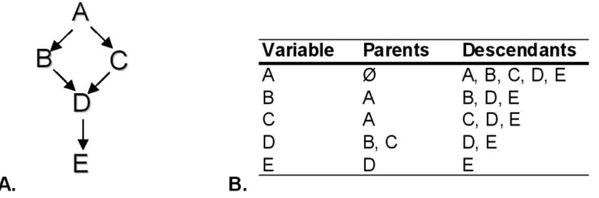
Figure 2.4: Representation and classification of the variables of a DAG G.

A. representation of the variables of a DAG G. B. classification of the variables of a DAG G.

Y.

For example Figure 2.4-A shows a representation of a DAG G and Figure 2.4-B a table with the classification of the variables of G. The DAG G has 5 variables (A, B, C, D and E) and the arrowheads between the variables are oriented edges. In G (Figure 2.4-A ) the set B, C, D, E is not causally sufficient, because there is another variable A, not included in the set, which is a direct cause of the B and D variables.

Conditional independence

the conditional probability of X given Z. In an other way we can say that X and Y are conditional, by independent when P (X|Y, Z) = P (X|Z)P (Y |Z). This mean that if X and Y are independent conditioned on the Z, then does not provide any information about Y once given knowledge of Z and vice versa [Spirtes et al., 2001]."

With only the causally sufficient criteria it is very difficult to find the best DAG from a given sample, since the number of possible DAGs is greater than the exponential of the number of observed variables. To reduce the number of possible DAGs, the Bayesian models use together other two different assumptions: Causal Markov Condition (CMC) and Causal Faithfulness Condition (CFC).

Causal Markov Condition (CMC)

The CMC states that given a set of variables whose DAG G represents the causal structure of these variables, each variable is independent of its non-descendents conditional on its directed causes (its parents in graph G) [Ramsey et al., 2012]. In particular in Figure 2.4-A, the CMC entails that if there is no edge between two variables A and D in a DAG G, then A and D are conditional independent on some subset of the other variables Z

(33)

The PC algorithm 23

(Z = B, C) (IP(D, A|B, C). In addition to the example between the variables A and D

there are other conditional independence relations entailed by CMC: IP(A, ∅|∅);

IP(B, C|A);

IP(C, B|A);

IP(E, {B, C, A}|D)

These relations may originate other conditional independence relations; for example IP(E, A|{B, C}). Another interesting consideration is that the CMC alone implies the

principle of the common cause. In fact if two variables X and Y are not conditionally independent on ∅(∼ (X, Y |∅)), then, according to the CMC, we have three possibilities: X is cause of Y, or Y is cause of X, or it exists a third variable that is the common cause of both X and Y (common cause).

Causal Faithfulness Condition (CFC or Stability Condition)

The CFC says that given a set of variables V and DAG G is the causal graph, DAG G is the true causal graph when it is the exact map of the distribution probability (P_V) of the variables in the set V. The probability distribution P entailed by a causal graph G satisfies the CFC if and only if every conditional independence relation true in P is entailed by the CMC applied to G [Zhang and Spirtes, 2008]. Under the CFC, conditional independence relations give direct information about the structure of the graph. In Figure 2.4-A with the CFC we can conclude that there is no direct edge between A and D if a statistical test indicates that A is independent of D conditional on Z(Z = {B, C}) [Zhang and Spirtes, 2008].

Assuming together the CMC and CFC it is possible to reduce the total number of DAGs, because they entail that conditional independency holds in the population if and only if the true causal DAG entails it by application of the Markov condition. To explain this concept we suggest to see the example present in the paper by Zhang and Spirtes [2008] (Figure 1 from paper Zhang and Spirtes [2008]). Given the DAG G in Figure 2.4-A, the CFC entails that IP(D, A|∅).

d-separation

There is a method to ascertain whether the CMC and/or CFC entail conditional in-dependence relation. The method is called d-separation (d means in-dependence), it is a graph-theoretical approach and is defined as follows.

Two variables X and Y are d-separated by a node set Z if and only if every path between X and Y is blocked. A path is blocked when there is an intermediate variable Z ∈ Z such that:

(34)

Figure 2.5: Different types of connections considered in the d-separation step.

1. the connection through Z is tail-to-tail or head-to-tail and Z has received evidence, or;

2. the connection through Z is head-to-head (or v-structure) and neither Z or any of Z’s descendants have received evidence.

The different types of connections are represented in Figure 2.5 in which each nodes of the different graph represent a variable and each arrowhead is an oriented edge. 2.2.1 Description of the PC algorithm

The PC algorithm reconstructs the causal structure of the variables described by the input data, starting from the assumptions of the Causal Markov Condition, faithfulness and causal sufficiency of a graph. The PC algorithm works by progressively removing the edges from a complete undirected graph built on the variables given in the input data, until no more edges can be deleted, according to a function that decides when to delete the edge. The graph so obtained is called skeleton and it is then oriented according to the d-separation rules.

The PC algorithm receives a set V of random variables in input and it works in three phases described in the pseudo-code in Figure 2.6 and in the representation in Figure 2.7. Phase 1: find the skeleton by deleting edges between independent variables The PC algorithm starts generating a complete undirected graph G’ from the set of variables V. Each node in the G’ is a variable of V thus from now the variables will be called also nodes. Subsequently, the PC algorithm starts to remove the edges in G’ testing the set of Adj(X). The idea is that if the set of independences is faithful to a graph, then there is not a link between variables X and Y, if and only if there is a subset S of adjacent nodes of X (Adj(X)) such that I(X, Y |S) [Spirtes et al., 2001]. For each pair of variables in the subset S, SX − Y will contain such a set, if it is found.

In particular in this Phase the PC algorithm uses the Partial Correlation Coefficient (PCC) to estimate conditional independencies. This parameter corresponds to the corre-lation coefficient between the dependent and independent variables when all the effect of the other variables are removed [Kalisch and Bühlmann, 2007].

(35)

The PC algorithm 25

(36)

Figure 2.7: PC algorithm schematic representation.

Phase 2: orient v-structures (head-to-head )

The orientation of the edges in G’ proceeds by examining sets of three variables {X, Y, Z} such that in G’ there are the unoriented links between X and Z and between Y and Z, but the link between X and Y does not exists. Then if Z is not included in SepSet(X,Y), the PC algorithm orients the edges from X to Z and from Y to Z creating a v-structure (head-to-head ): X → Z ← Y [Spirtes et al., 2001].

Phase 3: orient the remaining unoriented edges using rules

In the Phase 2 not all link between nodes are oriented, so in this phase the PC algorithm tries to orient the rest of the edges. To arrive to this aim it follows two rules:

- Cycles have to be avoided;

- New v-strucuters have to be avoided.

2.2.2 Proposed modifications of the PC algorithm

The PC algorithm as such was applied on gene expression data [Wimburly et al., 2003] and more recently it has been improved in its different Phases (Figure 2.8). In Phase 1 PPC was substituted with Conditional Mutual Information by Zhang et al. [2012] and

(37)

The PC algorithm 27

Figure 2.8: Schematic representation of the differences between the original PC algo-rithm and its modified versions.

the way in which the interactions between the nodes in the complete undirected graph are removed has changed [Wang et al., 2010]. In Phases 2 and 3 the way in which the edges are oriented was changed [Ramsey et al., 2012] [Ebrahimi et al., 2012]. In this section all these versions of the PC algorithm are reviewed.

Conservative PC algorithm (CPC) [Ramsey et al., 2012]

This algorithm aims to improve the PC algorithm in the orientation phase [Ramsey et al., 2012]. Ramsey highlights how the CFC assumption is formed from two com-ponents Adjacency-Faithfulness and Orientation-Faithfulness and how the causal Markov and Adjacency-Faithfulness conditions fail to orient the edges between the variables. An example shows this fact: consider three variables < A, B, C > where A is independent from C (A⊥ C) and A⊥C|B (A → B → C). In this situation the Causal Markov and Adjacency-Faithfulness are both satisfied, but Orientation-Faithfulness is not true for this triple.

The PC algorithm removes the edge between A and C, because A ⊥ C, but orients the edges in this way A→B←C, because B is not in SepSet found in Phase 1. To overcome this problem CPC algorithm in Phase 2 tests for each triple < A, B, C > which are the potential parents of A and C and not which are collider or non-collider. The Phase 2 in CPC is as follows. Let G a graph resulting from Phase 1, for each unshielded triple

(38)

< A, B, C >, check all subsets of A’s and C’s potential parents:

a. if B is not in any set conditioned on which A, and C are independent, orient A-B-C as A→B←C;

b. if B is in all sets conditioned on which, A and C are independent, leave A-B-C as it is;

c. otherwise, mark the triple as "unfaithful"by underlining the triple. This mean that there are possible different DAGs (A→B→C, A←B→C, A←B←C, A→B←C). Low PC algorithm (LPC) [Wang et al., 2010]

This algorithm was developed to make easier the application of the PC algorithm on large gene expression datasets. In fact the PC algorithm requires an high number of tests, because all possible combinations of the conditioning set have to be examined. For this reason LPC uses the procedures of the PC algorithm, but it executes only the low-order Conditional Independence (CI) tests. In fact, in LCP, the number of CI tests is limited by the k specified by the user. The limited order of the CI tests reduces the computational complexity, but does not improve the sample size to analyse. In fact both these two algorithms (PC algorithm and LPC) have the best performances with sample sizes of 100 and 1000 variables [Wang et al., 2010].

LCP has two phases: CI test and orientation phase. In the first phase a limited number of CI tests is executed in comparison to the PC algorithm. The number of CI tests depends on k and the value of k is given as input data together with the dataset D (e.g. microarray with n genes an m measurements). In the second phase (orientation phase), the neighbor number of connected node pairs is checked before applying orientation rules, because the neighbor number of connected nodes is linked with the k value. If the k value is equivalent to n-2, where n is the number of genes in the input dataset D, the LPC algorithm is equivalent to the PC algorithm. Therefore we can say that LPC is a generalization of the original algorithm (in the sense that it constrains the search with ao additional parameter) and not a variation.

Path Consistency Algorithm with Conditional Mutual Information (PCA-CMI) [Zhang et al., 2012]

PCA-CMI is a method used to infer GRNs from gene expression data based on the PC algorithm, but it substitutes PCC [Kalisch and Bühlmann, 2007] with Conditional Mutual Information (CMI) [Zhang et al., 2012].

Many GRN inference algorithms are based on Mutual Information (MI). They start by computing the pairwise MI between pairs of genes, then the MI values are elaborated to identify the regulatory relationships [Altay and Emmert-Streib, 2010] [Fernandes and

(39)

Methods for network expansion 29

Gloor, 2010]. In particular for two discrete variables X and Y , MI measures the depen-dency between X and Y and is defined as:

M I(X, Y ) = X x∈X X y∈Y p(x, y) log p(x, y) p(x)p(y) (2.6)

In case the two variables are independent p(x, y) = p(x)p(y).

MI presents the advantage of measuring non-linear dependency (more common in biology) and it is able to deal with thousands variables in the presence of a limited number of samples [Meyer et al., 2007]. The problem is that MI is able to test pairs of genes not considering that there are more than two co-regulators. To overcome this problem Zhang et al. [2012] have proposed Conditional Mutual Information (CMI). This parameter is able to identify the joint regulations by exploiting the conditional dependency between genes of interest. CMI, in fact, is the expected value of the Mutual Information between two variables X and Y, given that a third variable Z or a set of variables Z has occurred. It can be defined as:

CM I(X, Y |Z) = X x∈X X y∈Y X z∈Z p(x, y, z) logp(z)p(x, y, z) p(x, z)p(y, z) (2.7) where p(x, y, z) indicates the joint probability.

Limited Separator set in the PC algorithm (LSPC) [Ebrahimi et al., 2012] The LSPC algorithm aims to improve the way in which the edges are oriented in the Phase 2 and 3 of the PC algorithm. The main difference between these two algorithms is the choice of the separator set between the nodes of the graph G resulting from the Phase 1 of the PC algorithm.

PC considers as separator set of two vertices X and Y, all nodes that are present in the Adj(X) and Adj(Y). For LSPC the separator set is formed from all variables mostly repeated in the walks between X and Y. This method appears to improve the PC al-gorithm, because it reduces statistical errors in the step of edges orientation [Ebrahimi et al., 2012].

2.3 Methods for network expansion

GENESYS (GEnetic Network Expansion SYStem) [Tanay et al., 2001] is an algorithm that computes the fitness function of the LGN and then adds genes and relationships to find an expansion of the LGN that improves the fitness (Figure 2.9). In this system a biological network (or model) is defined from a set U of variables (e.g. genes or proteins), a set C of values (states) that the variables may attain, and functional dependence between

(40)

Figure 2.9: Overview of the GENESYS algorithm.

the variables is described by the function fv _{: C}|U |

→ C for each v ∈ U (the value of v at time t depends on the values of its input variables at time (t -1)). The prior knowledge is used at the beginning to describe a model space. This is defined by the quadruple (U, C, Fbio, Gbio), where U and C are the sets defined above, Fbio is the class of the candidate fv

and Gbio is a class of dependency graphs on U . Fbio and Gbio are used to limit the model

space and incorporate the prior knowledge of the LGN.

Fitness evaluation is a critical step to LGN expansion. The fitness function uses the idea presented in Liang et al. [1998] and it must perform well in term of sensitivity, precision and computing efficiency. In GENESYS there are two types of fitness: local and global. The local fitness function evaluates the fitness of the experimental data to the function fv of a single variables v, while the global function evaluates the overall network. Summarizing GENESYS starts from the LGN (G’) and outputs G”, namely the LGN expansion (G’⊆G”). The fitness value of G’ is determined and then one gene at a time (v ∈ U) is added to G’ and the new fitness is calculated. Only the genes that have an improvement of fitness respect to the raw G’ are selected and included in the G” [Tanay et al., 2001].

Hashimoto et al. [2004] developed the Growing algorithm that uses gene expression data to discover subnetworks of a large network, in which genes must to have two principal characteristics:

- genes of the subnetwork must be significantly related between them;

(41)

Methods for network expansion 31

Figure 2.10: Parameters generated by Growing algorithm

S is a gene of a LGN and Y is a set of all genes excluded S. Figure 2.10-a. represents the from impact of Y to S. Figure 2.10-b. presents the depiction of the to impact of Y to S. Figure 2.10-c. shows the measure of the strength of edge from genes external to S to Y (adapted from Hashimoto et al. [2004]).

subnetwork

In particular this method starts from a little initial group of genes (’seed’) and then adds new genes expanding the seed in a greater subnetwork. To reach this aim, the Growing algorithm proceeds modeling a GRN as a directed graph in which at each relationship between the variables is associated a coefficient of determination. "The coefficient of determination measures the degree to which a set of variables improves the prediction of a target variable relative to the best prediction in the absence of any conditioning observations"[Hashimoto et al., 2004].This means that the influence is used to measure the strength of a relationship and with the term σX(Y ) is indicated the sum of influences

of the genes in X on the set of genes Y. In particular if S is a a gene of a LGN and Y is a set of all genes excluded S then are measured three coefficient of determination:

- σf rom,S(Y): the collective strength of connection from the to the target set of genes

Y;

- σto,S(Y): the impact (strength of connection) of Y to S;

- σout,S(Y): the measure of the strength of edge from genes external to S to Y

Figure 2.10 represents the three determination coefficients that are computed from Grow-ing algorithm. Once computed σf rom,S(Y), σto,S(Y) and σout,S(Y) the algorithm combines