Agent-based simulation for renewable energy incentive design

Alma Mater Studiorum · Universit`

a di Bologna

SCUOLA DI INGEGNERIA E ARCHITETTURA

DIPARTIMENTO DI INFORMATICA - SCIENZA E INGEGNERIA CORSO DI LAUREA MAGISTRALE IN INGEGNERIA INFORMATICA

TESI DI LAUREA

in

SISTEMI INTELLIGENTI

AGENT-BASED SIMULATION FOR

RENEWABLE ENERGY INCENTIVE DESIGN

Candidato:

VALERIO IACHINI

Relatore:

Chiar.ma Prof.ssa

MICHELA MILANO

Correlatore:

Dott. Ing.

ANDREA BORGHESI

Sessione II

Anno Accademico 2013/2014

Abstract

Con questo lavoro s’intende proporre un nuovo approccio per modellare la diffusione di sorgenti rinnovabili di energia in ambito residenziale. A tal proposito, abbiamo deciso di adottare un modello basato ad agenti, dove gli agenti rappresentano le famiglie che risiedono nella regione in esame. Questo implica uno studio del territorio per determinare quali sono le caratteristiche delle famiglie che vi abitano. Il caso di studio `e quello del Piano Energetico della Regione Emilia-Romagna che mira ad aumentare la produzione di en-ergia soprattutto da fonti rinnovabili come biomasse e solare. Siamo partiti, quindi, dallo studio dei micro dati usati dalla banca d’Italia per ottenere le statistiche rilevanti sulle famiglie residenti in Emilia-Romagna. Questi dati ci hanno permesso di generare delle famiglie in modo artificiale e riprodurre virtualmente gli aspetti socio-economici della regione. Le famiglie generate per mezzo di un software sono collocate nel mondo virtuale associando ad ognuna di esse un’abitazione. Queste abitazioni sono acquisite analizzando i dati vettoriali degli edifici messi a disposizione dalla regione. Una volta predisposto il mondo virtuale, il modello ad agenti determina il livello diffu-sione simulando ogni anno la potenza installata dalle famiglie. La scelta di un agente d’installare un impianto `e influenzata dalle relazioni sociali, dalla condizione economica, dai benefici ambientali derivanti dall’adozione e dal periodo di recupero dell’investimento.

In this thesis, we propose a novel approach to model the diffusion of res-idential PV systems. For this purpose, we use an agent-based model where agents are the families living in the area of interest. The case study is the Emilia-Romagna Regional Energy plan, which aims to increase the produc-tion of electricity from renewable energy. So, we study the microdata from the Survey on Household Income and Wealth (SHIW) provided by Bank of Italy in order to obtain the characteristics of families living in Emilia-Romagna. These data have allowed us to artificial generate families and reproduce the socio-economic aspects of the region. The families generated by means of a software are placed on the virtual world by associating them with the build-ings. These buildings are acquired by analysing the vector data of regional buildings made available by the region. Each year, the model determines the level of diffusion by simulating the installed capacity. The adoption be-haviour is influenced by social interactions, household’s economic situation, the environmental benefits arising from the adoption and the payback period of the investment.

Contents

1 Overview 3

1.1 ePolicy . . . 4

1.2 Photovoltaic systems in Italy . . . 7

1.3 The Italian incentives for PV systems . . . 8

1.4 The Emilia-Romagna incentives for PV systems . . . 10

2 Background 15 2.1 Why an Agent-based model? . . . 16

2.2 Literature overview . . . 17 2.3 Previous work . . . 20 2.4 Development tools . . . 26 3 Proposed Model 29 3.1 Model description . . . 30 3.2 Network generation . . . 34

3.3 The household behaviour . . . 39

3.3.1 Economic utility . . . 43 3.3.2 Budget utility . . . 44 3.3.3 Environmental utility . . . 44 3.3.4 Communication utility . . . 45 4 Households Generation 47 4.1 The microdata . . . 50

4.1.1 The age class . . . 54

4.1.2 The education level . . . 55

4.1.3 The number of members and annual energy consumption 55 4.1.4 The income of a family . . . 56

4.2 The subdivision of families in social classes . . . 58

5 Model Simulation and Calibration 67 5.1 Model simulation . . . 68 5.1.1 Model calibration . . . 72 5.2 Results . . . 77

List of Figures

1.1 Policy making life cycle. . . 5

1.2 General scheme. . . 6

1.3 Evolution of the Italian PV market. . . 7

1.4 The Italian average solar radiation between 1981-2000 (GSE [2011]). . . 8

1.5 The Italian PV installed power GSE [2014]. . . 9

1.6 Trend of national incentives in Euro / kWh. . . 10

1.8 Comparison regional incentives Borghesi et al. [2013]. . . 13

2.1 Ant colony simulation - NetLogo world representation Wilen-sky [1997]. . . 17

2.2 Decision algorithmBorghesi [2013]. . . 22

2.3 Social interactions shown in the virtual world of NetLogo. . . 24

2.4 The simulator GUI. . . 25

2.5 NetLogo interface. . . 26

2.6 The virtual world of NetLogo. . . 27

3.1 Polygons of buildings contained in shapefiles. . . 32

3.2 Buildings preprocessing. . . 32

3.3 The population density of the LiveJournal Liben-Nowell et al. [2005] (Image from Liben-Nowell et al. [2005].) . . . 35

3.4 Comparison of rank-based model with homogeneous and het-erogeneous nodes. . . 36

3.5 The resulting network made only with homophilous links . . . 37

3.6 The resulting networks from varying p. . . 38

3.7 The communication utility values. . . 45

4.1 Generic S-curve. . . 48

4.2 The diffusion of innovations according to RogersWikipedia [2014]. . . 49

4.3 Age class frequencies. . . 54

4.5 Number of members frequencies. . . 57

4.6 Clustering of households. . . 59

4.7 Households generation steps. . . 61

4.8 Tool chain . . . 62

5.1 The NetLogo simulator screenshot. . . 69

5.2 World view after household are loaded. . . 70

5.3 Parameters tuning architecture. . . 74

5.4 Scheme of irace flow of information. . . 75

5.5 The worst-case execution time increasing the number of agents. 78 5.6 The installed capacity in Emilia-Romagna during the period from the first half of 2007 to the second half of 2012 . . . 79

5.7 The capacity growth rate in Emilia-Romagna. . . 80

5.8 Comparison of virtual world with 20 and 200 agents. . . 81

List of Tables

3.1 The possible values for TY EDI and STAT E . . . 33

4.1 Datasets available in the 2012 annual database . . . 51

4.2 Variables of RFAM12 . . . 53

4.3 Age Class: probability distribution . . . 55

4.4 Age Class: probability distribution . . . 64

4.5 Number of members: probability distribution . . . 65

4.6 Number of members: probability distribution . . . 65

4.7 Number of earners: probability distribution . . . 66

5.1 Model parameters. . . 82

Introduction

Public policy making is a set of complicated process with the purpose of addressing public problems that involve progressive and interactive environ-ment. Factors such as globalization make our society ever more complex, so the decision-making process must be adapted to the rapidly changing glob-alised world. The cities are becoming larger; therefore, the decisions taken by policy makers affect more and more individuals. This growth increases the chance that entities involved have conflicting interests that impact the achievement of goals. Policy makers must find a balance between the indi-vidual interests and the global objectives. It is not always simple because the amount of data to be examined, and the number of constraints to be considered can be very high. However, if they are assisted by tools that can provide predictive models, they could evaluate the consequences of their de-cisions.

The ePolicy project is a FP7 STREP project funded by the European Union, which is devoted to the development of Decision Support Systems (DDS) for assisting decision-makers to design socially accepted and sustain-able policies from the point of view of the environment. A Decision Support System may employ several techniques from different fields such as artificial intelligence, operations research, sociology, economics, etc.

ePolicy aims to help decision makers to evaluate social, economic and envi-ronmental impacts during the policy making life-cycle. Of course, when the problem is complex, and there are several requirements to be met, a DDS can aid to get the most benefit from the available data to formulate a plan able to produce the desired effect on the environment.

The ePolicy case study is the Emilia-Romagna Regional Energy plan. In Emilia-Romagna, the regional government has set a target to increase the production of renewable energy from sources such as solar and biomass. In this work, we focus on the solar energy and we propose a model for the residential PV system diffusion to evaluate public policies in this domain. Many researchers have found that the diffusion of an innovation is strongly

influenced by social aspects. In recent years, agent-based modeling has gen-erated significant attention as a tool for modelling social and individual be-haviours. Consequently, we propose an agent-based model that simulates the micro-based behaviour of households in order to evaluate and explain macro-level phenomena. In this work, we tackled the challenge of reproduc-ing the households behaviours when they decide to estimate the opportunity to utilize a PV system for their houses. Hence, an Agent Based Model is an intuitive approach to addressing the problem since we can concentrate on the factors that impact on the adoption of a PV system by analyzing the behaviour of individuals.

To test our model we recreate the Emilia-Romagna environment by analyzing data from the Survey on Household Income and Wealth (SHIW) provided by Bank of Italy [2012]. However, the process described is valid for any region or country.

The ultimate goal is to integrate our model in a DDS for the policy makers to evaluate alternative plans.

In the first chapter, we introduce the ePolicy project and the Emilia-Romagna Regional Energy plan case study. In Chapter 2, we provide the related works overview. In Chapter 3, we present in detail the proposed model. In Chapter 4, we describe the household generation. Finally, in Chapter 5 we present the model implementation, and we discuss the results obtained.

Chapter 1

Overview

Policy makers have to deal with extremely complex environments that rapidly change over time. Their decisions are transposed into a plan that is com-posed of several actions in order to archive the objectives. These plans may involve different entities and affect three pillars of sustainable development: economics, social iteration and environment. So, It is necessary to reach an appropriate balance between individual interests and the objectives of the plan.

The complexity of the environment makes it hard to assess the long-term effects of the plan. For this reason, the politicians must be able to get the most benefit from the available data to formulate a plan able to produce the desired effect. In addition, during the policy-making life cycle, policy makers can provide several alternative plans, so they need to find a way to evaluate different alternatives. A Decision support system (DSS) is often used to as-sist policy makers in under- standing the consequences of complex decisions.

DSS means a vast class of software tools that aim to help decision makers in case of complex problems by facilitating the analysis of large amounts of data and suggesting strategies and policies to be adopted. Over the past 30 years, there has been a growing interest in the DSS among AI researchers, which has led to incorporating artificial intelligence techniques to model prob-lems and simulate decision impacts. DSS architecture contains three essential components:

• the database or knowledge base,

• the model,

The model adopted in a DSS can be an agent-based model (ABM) when is necessary to simulate the actions and interactions of autonomous individ-uals. For example, political models cover more subjects who have different characteristics and interests. These subjects are represented by agents in an ABM model that interact with the environment and respond to changes that are made in accordance with the decisions taken by politicians.

An ABM allows us to model the problem by defining the behaviour of enti-ties involved. Normally, the behaviour of individuals is very simple but the emergent behaviour from the interaction of many agents can be complex to be modelled directly. So, ABMs are useful to understand emergent phenom-ena by simulating the micro-based behaviour of agents.

The ePolicy project was created to demonstrate the contribution that the DSS can give to politicians to make decisions when the problem is complex, and there are several requirements have to be met. The purpose is to provide an open source tool, easy to use and that it can supply useful indications for the user.

1.1

ePolicy

The ePolicy project aims to support policy makers in their decision process and to evaluate of social, economic and environmental impacts during policy making. The project is coordinated by the University of Bologna, and it involves nine partners from academia, research institutions, regional govern-ments and the private sector of the European Union.

Policy makers have to deal with complex problems that have a large num-ber of variables and constraints which concern different environmental, social and economic aspects.

An important factor that can help policy makers in their decisions is the feedback from citizens. Through social networks, blogs and other means, cit-izens can judge the decisions and contribute to the creation of policies. So, decision makers have the opportunity to know the social impacts through opinion mining on e-participation data.

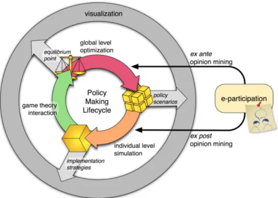
We can summarise the policy making life cycle as shown in Figure 1.1: • the global level optimization produces plans and scenarios for policies

taking into account the objectives, the financial aspects and the envi-ronmental and social impacts on a large scale.

• The individual level simulation reproduces the social behaviour based on personal opinions.

Figure 1.1: Policy making life cycle.

• The integration between the overall goal and personal goals is done using the techniques of game theory.

• The feedbacks and opinions of the entities involved are obtained using opinion mining techniques.

• Tools for visualization of the results can help decision makers.

Figure 1.2 shows the general scheme of the system. At the base, we have the involved entities in the decision whose opinions are used in the policy making life-cycle. Above the entities there is the individual level simulation. This level consists in an ABM that simulates the behaviour and interaction of the individual entities. At the top is the global level optimization that tries to find a solution by taking as input financial aspects, impact, constraints and objectives.

Thus, the ePolicy project aims to equip policy makers with integrated models, optimization, visualization, simulation and opinion mining tech-niques that improve the outcomes of complex global decision making. The ultimate goal of the project is to provide tools that are capable of evaluating

Figure 1.2: General scheme.

several alternative plans and to provide for each of them an analysis of costs and benefits. These tools make use of the most advanced techniques of ar-tificial intelligence for solving constraint satisfaction, optimization, planning and other problems.

These ideas have been used to solve a particular problem: the energy plan-ning in Emilia-Romagna. The regional government has set the target to increase the production of renewable energy from sources such as solar and biomass. Since 2009, these are also Italian and European goals with the Directive 2009/28/EC of the European Parliament and of the Council of 23 April 2009 on the promotion of the use of energy from renewable sources

(European Commission [2009]).

ePolicy seeks to develop a software system capable of supporting decision makers in the development of an incentive system to increase the installed number of photovoltaic systems with minimal effort for the region.

To illustrate the problem, in the next sections of the chapter, we are going to introduce the situation of photovoltaics in Italy.

1.2

Photovoltaic systems in Italy

After the introduction of national incentives, the Italian photovoltaics (PV) market has experienced a remarkable growth. The number of PV systems has more than doubled each year from 2008 to 2011. However, the growth rate in 2012 was lower than 2011, because in the 2012 the number of installed systems was 45% more than 2011. The installed power increased from 87 MW in 2007 to 16.420MW in 2012. The power has grown more than the number of installed systems because large plants came into operation, but the average size of the plants has decreased from 38.7 kW in 2011 to 34.3kW in 2012. The phenomenon is linked to a reduction in the installation of large systems determined by Legislative Decree 1/2012, which has limited the size of plants installed on the ground. Plants that came operation in 2012 have

Figure 1.3: Evolution of the Italian PV market.

an average power equal to 24.6 kW that is lower than the plants installed in 2010 and 2011. During 2012, the operating power has increased to 3.646 MW.

The distribution of power among the Italian regions is not homogeneous. According to data from the Gestore dei Servizi Elettrici S.p.A. (GSE), the highest number of plants is found in the North, especially in Lombardia and Veneto (Figure 1.4). This fact is a strange because the number of installed PV systems is much higher in the North, although the irradiation level is lower than other areas of the country. In addition, most of the installed systems in the North belong to households and are characterized by small capacity. In the southern regions of Italy, a very substantial part of the power is installed on the ground. This fact could suggest that more aspects other than pure geographical or economical one should be taken into account.

Figure 1.4: The Italian average solar radiation between 1981-2000 (GSE [2011]).

1.3

The Italian incentives for PV systems

The Italian mechanism to encourage the installation of solar systems is called “Conto Energia” (CE). This mechanism, that rewards with tariffs the energy produced by photovoltaic systems for a period of 20 years, became

opera-tional in 2005 (First CE). Since then, the incentive scheme has been renewed five times with a series of adjustments and changes. Unlike in the past, where the incentive for the production of energy from renewable sources was done by contributing non-repayable money, the CE introduces a funding system to increase earnings from energy production. A necessary condition to ob-taining the tariffs is that the system must be connected to the grid and must have at least 1 kW of peak power. The CE does not provide an incentive for stand-alone systems.

The main changes introduced by the Second CE was the application of the incentive fee on all energy produced and not only on that produced and con-sumed in place, the simplification of bureaucratic procedures for obtaining the incentive and the differentiation of rates based on the type of architec-tural integration.

Until the fourth CE, the feed-in tariff was applied on all the energy produced by the plant. The fifth CE divides the tariff into two parts: the inclusive tariff applied to the energy fed into the grid and the self-consumption tariff applied to the energy consumed on site.

Figure 1.5 shows the CE results from 2007 to 2014. The CE considers two

Figure 1.5: The Italian PV installed power GSE [2014].

different support schemes. The first scheme is a net metering plan for plants with a capacity of less than 200 kW. In this schema, PV-generated electricity not consumed is fed into the grid. Then it can be retrieved by the household when needed. Besides the payment for each produced kWh of electricity, the GSE provides a contribution that guarantees the repayment of a portion of the expenses incurred by the family for getting electricity from the grid.

In the second scheme, the electricity produced in excess is sold to the GSE, which guarantees a minimum purchase price. In this case, the GSE operates as an intermediary between the producer and the market.

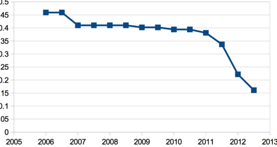
The following chart that was obtained by averaging the tariffs for all power classes shows the trend of national incentives in Euro / kWh for the period 2006-2012. As you can see, from 2007 to 2010 the national feed-in tariffs

Figure 1.6: Trend of national incentives in Euro / kWh.

have declined gradually with the further reduction in the second half of 2011 and the first half of 2012 (Fourth CE) and again in the second half of 2012, with the Fifth Conto Energia.

1.4

The Emilia-Romagna incentives for PV

systems

The Emilia-Romagna region has been chosen as a case study by the ePolicy project. The trend of solar installations in the area is shown in the following charts. In Emilia-Romagna, there was a reduction in the percentage of in-stallations between 2011 and 2012. This trend is the same as found in other Italian regions.

Although the incentive rate has been decreasing over the years, the number of plants instead has increased until 2011. So, the reduction of plants in the 2012 is not only due to the economic factor but also by other factors. An explanation can be found to the limitation that the fourth CE imposed on ground installations that are larger than those on the roof.

(a) KW of installed PV power in Emilia-Romagna [KW].

(b) Number of installed PV in Emilia-Romagna.

that the region can put in place to provide a further incentive for the instal-lation of PV (Borghesi et al. [2013]):

• Investment Grants - incentives are given as a grant, and no money is returned to the Region. The grants that are provided represent a proportion of the total plant cost. The financial requirement for the Region would be front-loaded as funds would need to be provided in advance of equipment installation.

• Fiscal Incentives - incentives are given as soft loans, including longer repayment periods or interest holidays. Again the financial require-ment on the Region would be front-loaded as funds would need to be provided in advance of equipment installation. In this case the loan would, eventually be paid back to the Region.

• Interest funds -incentives are given to pay all or part of the interests on bank loans taken in order to purchase PV equipment. Again no money is returned to the Region. In this case the financial burden on the Region would be spread over the lifetime of the loans that are likely to be a number of years.

• Guarantee fund - the Region provides a guarantee to the bank provid-ing the loan to an investor who is purchasprovid-ing PV equipment that the loan will be repaid. This fund provides security to the bank that is, therefore, more likely to approve the loan request and to charge a lower interest rate than would otherwise be the case.

The goal is to find the best incentive that allows the greatest increase in installations with less effort. This intention requires a simulator able to re-produce the behaviour and interaction of families. This simulator must be integrated into a system capable of providing the right support for policy-makers to find the best solution to achieve the objectives. One important

thing is that the simulator must provide a budget, for each type of incentive considered, that the region must allocate in order to obtain the desired in-crease of PV power.

The version of the software, which makes use of the model developed by Borghesi [2013] for the diffusion of PV systems, compares these incentives. The results are shown in the article Borghesi et al. [2013]. The purpose of Borghesi et al. [2013] is to identify the relationship between the capacity of PV systems installed and the budget allocated for regional incentives. Each regional incentive was individually simulated multiple times for each value of the regional budget from zero toe40 million, in steps of e1 million. To learn the functions that govern the relationship between the available budget and the installed capacity, Borghesi et al. [2013] have used machine learning techniques. Figure 1.8 shows the simulation results. As you can see, the regional incentive that provides the greatest increase in capacity is the interest fund. In fact, the curve that relates the installed capacity and the available budget is almost always above the other.

The Interest Fund incentives are the ones that require the least amount of money for each installation. So, with this incentive mechanism the region can satisfy the vast majority of requests from citizens. Furthermore, the possibility of paying in installments allows the family to deal with the initial price of the system.

Chapter 2

Background

In recent years, Agent-based model has become increasingly popular as a modelling approach because it provides a systematical way to model the environment. This kind of model is mostly used in social science research to study how the environment evolves over time. In particular, ABMs are adopted to study the diffusion of an innovation that is strongly influenced by social aspects: people exchange information on the new idea (Rogers [2003]). This information reduces the uncertainty about the innovation and influences people in the decision whether or not adopt the innovation. An ABM can be used to model this information exchange between potential adopters to evaluate how the innovation spreads between them in different situations. For instance, a company can use it to determine the amount of advertising budget that should be allocated to reach the desired rate of spread.

For the reasons mentioned above, in this work we adopt Agent-based simu-lations for modelling the entities involved in a plan. In this context, entities can be individuals, companies, government agencies, etc., and then our model tries to reproduce their behaviour and how it is affected by economical, social and environmental factors.

Recently, ABMs were applied to model the diffusion of residential PV sys-tems and evaluate the effectiveness of incentives. In this case, agents are households whose behaviour is represented by the decision to buy or not a photovoltaic system. An agent who has installed a plant increases the possi-bility that agents in the same neighbourhood decide to make the same choice. This interest in the ABMs has led to the emergence of specific programming languages. These languages include constructs that facilitate the definition of the kinds of agents involved, their behaviour and their interaction. For our simulator, we used the development environment NetLogo (Wilensky [1999]). NetLogo provides a multi-agent programmable modelling environment that make easy to implement the model equipping it with GUI. The GUI allows

the user to interact with the model parameter to explore the effects on the virtual world.

This chapter provides the reasons that led us to use an agent-based model for modelling the environment and an introduction to the related works.

2.1

Why an Agent-based model?

An agent-base model (ABM) is a computational model used to simulate the actions and interactions between agents. Using an ABM you can model the individual entities that populate the virtual world independently. Generally, entities are very simple, if taken individually, but their actions and interac-tions can reproduce complex phenomena.

ABMs provide a systematic approach for the development of a model. In fact, it starts with the identification of entities that are part of the model. Then development proceeds by determining the actions that an agent can perform to interact with and manipulate the environment around them. Once the environment where the agents operate has been defined the model is com-plete. The global behaviour is not specified in the model but arises from the behaviour of mere agents.

Of course, there are techniques that model the system at the macro level. These models are called macroscale models while the ABMs are a kind of mi-croscale model. ABMs are easier to implement because simple behavioural rules leads each agent. In addition, the whole is greater than the sum of the parts (Bonabeau [2002]).

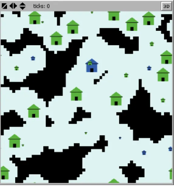
A field of application of ABMs is the simulation of natural systems. An ex-ample of natural systems is the ant colonies (Colorni et al. [1991]). The ants are the agents and follow simple rules. They randomly search for food, and upon finding it they return to the hive, dropping a pheromone trace which marks their trail. If another ant finds a pheromone trail, it will likely follow it. Ants that find the food source reinforce the pheromone trace in the track and as time passes the pheromone traces evaporate.

Figure 2.1 shows the NetLogo virtual world where the ants carry food back to the nest along the established route.

The emergent behaviour of the system is that the ants can find the short-est path to reach the food. The evaporation of the pheromone encourages the formation of a short path because in the long ones the pheromone has more time to evaporate.

In the case study of ePolicy, an ABM is used to model the spread of solar systems in the region Emilia-Romagna. As agents we considered the families inhabiting in the Emilia-Romagna Region and which could be interested in

Figure 2.1: Ant colony simulation - NetLogo world representation Wilensky [1997].

the adoption of a PV system. The philosophy of the ABMs is K.I.S.S. (”Keep it simple, stupid”), and then the families are modelled in an easy way. In the proposed model, the agents calculate a utility function that determines the level of desire to adopt a PV system.

The researchers showed that the diffusion of innovation is strongly influenced by social aspects. People who have adopted an innovation spread their ex-periences, strengths and weaknesses, related to the innovation (Abrahamson and Rosenkopf [1997]; Chatterjee and Eliashberg [1990]). This communica-tion reduces uncertainty about the innovative product and determines the degree of penetration among potential adopters. Thus, the ABMs can be used effectively to model this social aspect which is one of the main elements that drives the diffusion of photovoltaic systems.

2.2

Literature overview

Many scholars have tried to model the diffusion of innovations. Rogers M. claims that the diffusion of innovation is related with the communication

between individuals, and the adoption is affected by the exchange of infor-mation. So, the innovation diffusion is a social process, and the commu-nications between people play an important role in the decision to adopt or not the innovation. In this direction, Abrahamson and Rosenkopf [1997] have implemented a threshold model based on “bandwagon effect”. In this model, the increase of the adopters generates new information on innovation that produces a greater pressure on people who have not yet adopted the innovation. The potential adopters make an estimate on the profitability of innovation. However, they are unsure about the correctness of the assess-ment, so other people who have already adopted the innovation influence their decision. Abrahamson and Rosenkopf [1997] express this relationship with the following equation:

Bi,k = Ii+ (Ai· Pk−1) (2.1)

Where Bi,k is the bandwagon assessment of innovation at cycle k of the

poten-tial adopter i, Ii is the assessment of profitability of innovation and Ai· Pk−1

is the bandwagon pressure. Pk−1is the amount of information received that

create the bandwagon pressure after k − 1 cycles and Ai denotes how much

the potential adopter i weights this information. Also in the model proposed by Chatterjee and Eliashberg [1990], people influence each other in their de-cisions. The decision is based on two attributes: price and performance. The price is known, but the performance is uncertain and based on the percep-tion that the potential adopter has of the innovapercep-tion. This uncertainty is reduced over time because the potential adopter receives a stream of infor-mation about the performance by word-of-mouth from adopters.

Many of these models are agent-based model (ABM) where the agents are connected to form a small-world network. The small-world model was proposed by Duncan J. Watts and Steven Strogatz in their joint 1998 Nature paper. It consists of a random graph algorithm that produces graphs with the small-world properties that have high clustering coefficient and low mean-shortest path length. To prove the validity of this model, Stanley Milgram and other researchers conducted the small-world experiment to examine the average path length for social networks of people in the United StatesTravers and Milgram [1969]. This research has shown that human society is a small world network.

In a small-world network, most of the nodes are not neighbours, but most of them can be reached from every other by a small number of hops. In particular, the average distance between two nodes grows proportionally to the logarithm of the number of nodes in the network (Watts and Strogatz [1998]). This characteristic is obtained from a ring lattice where each node

is directly connected to k immediate neighbours by random rewiring of some links.

Recently, some researchers have proposed specific models to describe the adoption of solar panels for domestic use. Zhao et al. [2011] have proposed a two level threshold ABM where agents are households. The low level is devoted to simulating each agent electric consumption and to provide and estimated payback time. Instead, the high level is related to model the customers’ behaviour on adopting PV systems for 20 years. The adoption is based on four factors: payback period, household income, neighbourhood and advertisement. These factors are combined to define the desire level of a certain household for adopting a PV system. The model uses the following linear equation:

Di = wppfpp+ wincfinc+ wneifnei+ wadvfadv (2.2)

Where Di is the desire level for the household i and wpp,winc, wnei and wadv

are the weights associated with factors fpp,finc,fnei and fadv. Each factor

is represented by a value between 0 and 1. In order to have a desire level between 0 and 1, the next constraint is added:

W = wpp+ winc+ wnei+ wadv = 1 (2.3)

If the desire level of the household exceeds the threshold, the household installs a PV system.

Palmer et al. [2013] proposed an ABM to estimate the PV system diffusion among households living in Italy. In particular, each agent represents a household characterised by eight attributes. These attributes are used to assign a cluster to each family. The clustering is based on Sinus Milieu R

groups formed by people that share similar characteristics. Moreover, agents are linked to form a small world network in such a way those who are in the same cluster are more likely to be linked together. The decision to invest on PV system is based on desire level proposed by Zhao et al. [2011]. The difference is that the weights used for each factor depend on the cluster of the family. Thus, people in the same conditions weight the various factors in the same way. The desire level (or utility function) U (j) is calculated as:

U (j) = wpp(smj)upp(j)+wenv(smj)uenv(j)+winc(smj)uinc(j)+wcom(smj)ucom(j)

(2.4) Where smj is the Sinus Milieu R group. As before, upp(j) is the payback

period factor, uinc(j) is the household’s income and ucom(j) represents the

added to take into account the environmental benefit of investing in a PV system.

Robinson et al. [2013] has proposed a model that uses a geographic in-formation system (GIS) along with an ABM to study the diffusion of solar systems in order to take into account the real topology of the area of interest. In this case, an agent is mostly influenced by agents who have a similar opin-ion on technology. Each agent i has the variable xi that represents its opinion

and the variable uj that represents its uncertainty. If an agent i has in its

social network agents who have installed a photovoltaic system, the agent i randomly selects one of them, agent j, with a probability proportional to the similarity of opinions on technology. The relative agreement is calculated as follows:

hi,j

ui

− 1 (2.5)

where hi,j is the overlap of views between i and j and it is equal to:

hi,j = min((xi+ ui), (xj+ uj)) − max((xi− ui), (xj − uj)) (2.6)

The agent i opinion increases/decreases according to hi,j. The opinion and

the uncertainty of an agent j are updated as follows:

xj = xj+ µ((hij/ui) − 1)(xi− xj) (2.7)

and

uj = uj+ µ((hi,j/ui) − 1)(ui− uj) (2.8)

where µ is the constant that controls the speed of convergence of opinions. Next, if the intention of the agent i is greater than a threshold, the system is compatible with its roof, the payback period is below the threshold and its budget can cover the expense, then the agent i installs the PV system. In the next session, we introduce the previous work that is the basis of the proposed model.

2.3

Previous work

The original ABM, proposed by Borghesi [2013], simulates the diffusion of PV systems in Emilia-Romagna to understand the impact of regional incentives for a period between the first half of 2007 and the second half of 2036. During

the simulation, new PV systems are installed by households until the second half of 2016 and the simulation proceeds until 2036 to cover the average life of a PV system that is estimated to be 20 years. On each step until the second half of 2016, new agents are added to the environment in a random position across the virtual world. The number of agents created each year is a parameter of the model. Each agent is characterized by:

• ID - an integer value used to distinguish agents;

• Roof area - the surface available for installing a PV system; • Budget - the amount available for purchase a PV system;

• Average annual consumption - the average electricity consumption per year;

• The percentage of consumption that the agent wants to cover; • Obstinacy - the agent’s desire level to purchase a PV system.

Only agents that know PV technology perform an assessment, the others do not become part of the system. The knowledge diffusion is defined by the initial percentage of agents who are aware of PV technology and the yearly increase of this rate. The increase could vary following a linear relationship, a quadratic one or a cubic one. In the model proposed by Borghesi [2013], the impact of knowledge diffusion is very high: the annual installed power varies significantly by changing this parameter. Another factor that considerably impacts the simulated results is the annual increase of the percentage of agents who knows about PV panels. Using the different models for the growth of knowledge change how fast the knowledge increase each year. Thus, when the agent is generated, the simulator determines, using a simple probabilistic model, if he knows or not the technology of solar panels, and if he knows, he makes an assessment. First, the agent establishes the annual kW that PV system must generate with the following equation:

annualkW = (Average annual consumption·percentage of consumption) (2.9)

Hence, the size of the system:

dimension = annual kW

Accept Loan? Accept Loan? Decrease Size? Decrease Size? Knowledge Diffusion Knowledge Diffusion Estimate ROE Estimate ROE Feasibility Study (Physical/Financial Constraints) + Social Component (Agent environmental concern/neighbours) + Incentives Forecast Feasibility Study (Physical/Financial Constraints) + Social Component (Agent environmental concern/neighbours) + Incentives Forecast Exp.ROE >= Min.ROE DIE DIE INSTALL PANEL INSTALL PANEL Agent “knows” PV tech. Agent “knows” PV tech. Yes No Yes No No No No Yes Yes Insufficient Budget All Feasibility Conditions Met Insufficient Roof Size No Feasibility Conditions Satisfied

Figure 2.2: Decision algorithmBorghesi [2013].

Where m2Kwp is the constant that relates the square meters with kWp of PV system. Once the size is determined, the price is calculated as follows:

The simulation is subdivided in steps that represent every single semester. In each semester, the simulator creates a user-defined number of agents, which are spread in the virtual world. After the creation of an agent, the system proceeds to estimate its intention to buy or not a PV system. As shown in Figure 2.2, the steps that lead to the decision are:

1. If the PV system is smaller than the size of the roof and its cost is lower than the budget, the agent evaluates the possibility of increasing the dimension of PV system;

2. If the system is bigger than the size of the roof and its cost is greater than the budget, the agent leaves the system;

3. If the size of the plant is greater than the surface, but the budget is sufficient the agent evaluates to scale down the power of PV system; 4. If the size of the system is less than the available surface, but the budget

is low, the agent evaluates the possibility to take out a loan.

In all cases, except in step two, the obstinacy of agent comes into play. The obstinacy of an agent increases with the growth of the number of neighbours who have installed a PV system. Agent’s neighbourhood consists of agents whose distance is less than the radius specified as a parameter.The social interaction between agents is modelled as the sensitivity of an agent to the influence of neighborhood. The sensitivity is a value that can vary and a higher values correspond stronger influence from the neighbourhood. Thus, we expect higher probability to install PV panels.

In summary, each agent has a value (a component of obstinacy seen above) that represents how significantly his behaviour is influenced by friends, trying to reflect the human tendency to follow the group choice. In particular, the decisions of each agent are modified by his sensibility to neighbour’s behaviours and the size of the area of influence, which is the radius that determines the circular area within the choices made by an agent may affect the actions of others. Figure 2.3 shows the NetLogo virtual world where the areas of influence are denoted by almost circular shapes centered on the houses that represent the agents.

In step 1, if the obstinacy is greater than 50%, the agent evaluates the possibility of increasing the PV system dimension. The dimension is set to the roof area, and if the budget is greater than the new price, the system is installed. Otherwise, the PV system is realized with the dimension calculated by the equation 2.10. In step 3, the agent accepts to scale down the power if the following constraint is verified:

Figure 2.3: Social interactions shown in the virtual world of NetLogo.

Instead, in step 4, the agent takes out a loan to cover the price if the next constraint is verified:

(P V system price − budget) ≤ (budget · obstinacy) (2.13) In both step 2 and 3, if the condition is not met the agent leaves the system. Otherwise, if all the above conditions are met, the agent estimates the ROE of investment. The assessment takes into account the PV system cost, the national incentive (GSE price), the regional incentive, the energy price and eventually the mortgage payment. The gains are calculated as the sum of

the bill savings and the sale of energy. Thus, an agent installs a photovoltaic system if the estimated ROE is greater than a threshold.

Besides parameters with significant influence such as knowledge diffusion and agents interaction, the model has parameters that affect the results in a less evident way, such as almost all the pure economic factors. As an example of an economic parameter with a lesser influence than the previous ones is the annual reduction of the cost of PV panels. This parameter represents the reduction of prices due to technological advancements and in the model is a variable given as a percentage that tell how much each year the cost of a panel decreases in comparison to the last year price.

The plant comes into operation in the same year and semester in which the agent makes a decision. Each PV system is characterized by year, semester, type, technology, power band and dimension. The energy that can produce a PV system is linked to the geographical location and orientation. As a simplification, for all PV system the orientation is assumed to south with tilt to 30◦.

Figure 2.4: The simulator GUI.

Once the execution of the simulation is finished, the GUI (Figure 2.4) shows a variety of information, many of them are attractive to investors, such as PBT and the average ROE for different semesters, others are useful to determine the characteristic of the simulated environment, such as the overall installed power, the total expenditure for the installation and the percentage of plants built.

2.4

Development tools

NetLogo (Wilensky [1999]) is a programmable modelling environment for simulating natural and social phenomena. The development environment is written in Java to be as independent as possible from the execution platform. The NetLogo language inherits and extends the features of multi-paradigm programming language Logo, made in the 60s at the Massachusetts Institute of Technology and characterised by its derivation from Lisp and the numer-ous applications in the field of education. The code that defines agent’s be-haviours is interpreted, so the model is not previously compiled into machine-language instructions.

The development environment consists of a graphical interface organised into three tabs: interface, info and code. The interface tab allows you to interact intuitively with the parameters that govern the model or perform actions through the use of buttons, sliders, or other items. This interface has the important function of showing the movements of the agents inside the vir-tual world and present during and after the simulation information in the form of charts, tables, etc. The info tab provides information on the model. Besides the info tab there is the section that relates to the code, which de-fines the behaviour of the entities that act in the virtual world. The code of the simulation resides all within a single list, and it is divided into several procedures. The agents, entities that can execute instructions, can be of four

types (Figure 2.6):

• Patches are organized in the grid to form the two-dimensional world; • Turtles move on this grid;

• Links are agents that connect two turtles;

• The observer oversees everything that happens, and it does everything that the turtles, links and patches cannot do.

Figure 2.6: The virtual world of NetLogo.

All agents can issue commands and procedures. A Command is a Logo instruction that an agent can perform to interact with others or to change its state. Instead, the procedures combine a series of commands in a new command.

In NetLogo, you can define breeds of turtles or links. Breeds allow you to divide agents and then define specific behaviours. For each type of agents, NetLogo provides an agentset that is a set of agents. An agentset allows ex-ecuting a series of commands to all or part of the agents in it. The agentset makes the code cleaner and more readable and facilitates the implementation of the model.

NetLogo provides two ways to update the simulated time: continuous or tick-based. The continuous mode updates the view a user-specified number of times per second. In tick-based models, an update occurs when the in-struction tick is executed. The continuous mode is more expensive because the updates are more frequent than the tick-based, resulting in greater use of resources. Also, since we are not able to manage when the model needs to be updated, the system may be in an inconsistent state when the simulation is stopped. Usually, the continuous mode is used for debugging because it allows checking in detail how the system evolves.

NetLogo makes it possible to perform many times a simulation and try differ-ent configurations of parameters to study the results. These results help to understand the emergent behavior due to the interaction of multiple agents.

Chapter 3

Proposed Model

This chapter describes the model proposed to simulate the diffusion of photo-voltaic systems. First, we proceed to investigate the related works, and then we are going to explain our solution to address the problem. In Italy has been put in place a national feed-in-tariff to stimulate the installation of PV systems. The region may apply a greater incentive to reach the 2020 target. The 2020 climate and energy package (European Commission [2009]) is an ambitious goal that aims to arise the share of EU energy consumption pro-duced from renewable resources to 20% before 2020. We consider four types of incentives that a region can implement for the adoption of PV systems:

• Investment Grants - money given by the region to a household so that it can invest in PV system;

• Fiscal Incentives - the region provides loans with low-interest rates; • Interest funds - the region pay part or all of the interest that the citizen

owes the bank;

• Guarantee fund - the region guarantees for those who want to take a bank loan. In this way, it is easier to get a loan.

In this work, we propose a tool for decision makers to evaluate these regional incentives. This tool requires a model that can predict the photovoltaic system diffusion among households. Therefore, we propose an agent-based model that simulates the micro-based behaviour of households in order to evaluate and explain macro-level phenomena. We focused mainly on families living in the region of Emilia-Romagna, but the process described below is valid for any region or country.

The goal of proposed simulator is to recreate the phenomena of PV system distribution, attempting to create a relationship among families to simulate

the diffusion of knowledge about the advantages of PV systems. These fam-ilies are placed through an actual density distribution on the virtual world. The simulation consists of two major phases: the configuration phase, where the simulator creates a virtual word that has features similar as possible to the real and the running phase where the system simulates the degree of adoption among the agents from the first half of 2007 to the second half of 2016.

In the configuration phase, households are generated. Each family is charac-terized by attributes such as income, age and education level of main income earner. The distributions of these attributes are obtained from the Survey on Household Income and Wealth (SHIW) provided by Bank of Italy [2012]. After that, each family is assigned to a social group composed of families who share similar conditions in order to have a similar behaviour on families that have similar wealth. Then, each of them is assigned to a building on the simulated world. These buildings were obtained by processing the shapefiles that the region provides on the website Emilia-Romagna [2014].

In the running phase, the simulator simulates the behaviour of households for a period from the first half of 2007 to the second half of 2036. Annually, each household proceeds to evaluate the adoption of PV system. In the model, the desire level for adoption of a PV system is estimated by means of a utility function that an agent calculates according to its characteristics. In our sys-tem every agent makes the best choice that is the PV syssys-tem that maximise its reward, in terms of the production and saving, because we want a generic simulator that can simulate different incentive. Thus, we do not kwon what is the best size of PV system a priori. Normally, families ask for advice from installers and consultants, so it is fair to assume that in making the decision a family makes the best choice. So, an agent estimates the optimal size of the PV system that guarantees the best return on equity (ROE).

If the value of the utility function exceeds the threshold, the agent installs the system. The utility function takes into account the income of the family, the payback period, the environmental benefits and the relationships with other families. These factors are weighted differently depending on the social group of the family. The weights for each group are determined by calibrating the model on real data over the 2007-2012 period.

3.1

Model description

In the proposed model, the agents represent the families living in the region of Emilia-Romagna. As already mentioned, the simulation is divided into

two phases. In the first phase, the households are generated. In the second phase is simulated the behaviour of the agents.

The generation begins by establishing for each household age class, education level, income, family size and budget. The distribution of each attribute is obtained from the SHIW data. In addition, each agent is assigned to a class that represents a group of people who share the same characteristics. This class influences the value of the utility function.

The budget of a household for the purchase of a PV system is derived from its income by the equation:

budget = eincnorm_{ap (3.1)}

where:

• ap is the average price of a PV system;

• incnorm is normalized income obtained from log

income − m v ;

• v =√2Φ−1(Gini + 1

2 ) is the lognormal distribution variance;

• m = log minc−

1 2v

2_{is the lognormal distribution mean.}

The equation states that if a family has the income around the mean, the family expects to pay the average PV system price. Otherwise, if the family income is lower or higher than the average, the family will aim to spend less or more for a PV system.

Then each family is associated with a building on the territory of the region taking into account the family size and income. Buildings are sorted by their roof size and families with high income and high number of mem-bers are assigned to the bigger ones. The buildings are obtained from Ersi shapefiles that Romagna region has released on the website Emilia-Romagna [2014].

The Shapefile or simply shapefile is a geospatial vector data format for geo-graphic information systems software. This format was developed and reg-ulated by ERSI, in order to improve interoperability between GIS systems. The shapefile describes points, polylines and polygons, which represent ob-jects placed on the map. Normally, ”shapefile” refers to a set of files with the extension Shp, Dbf, Shx and others that share the same name. As shown in Figure 3.1, the shapefiles provided by region contain a polygon for each building detected. Since the simulation requires only the positions and the

Figure 3.1: Polygons of buildings contained in shapefiles.

areas of the roofs, it was necessary to preprocess these files. Using QGIS (QGIS Development Team [2009]), a free and open source Geographic Infor-mation System (GIS), it was possible to manipulate these shapefiles. QGIS is a very powerful tool, which allows to capture, store, manipulate, analyze, manage, and present all types of geographical data. It was possible to calcu-late the area and the centroid of the vertices for each polygon.

Figure 3.2: Buildings preprocessing.

Figure 3.2 shows the preprocessing performed with QGIS. For each poly-gon, we calculate the area, and we keep only the centroid (the point in purple)

of vertices (the points in red). In the model, the polygon area is assumed as roof area, and the centroid is assumed as the location of the house on the map.

As said before, shapefiles alone are not sufficient to describe the buildings because they contain only the geometries. So, the region also provides the dbf files that describe each building with several attributes, including the TY EDI that specifies the type of the building and STAT E, which indicates the state of the building.

TY EDI D TY EDI 1 Generic 4 Bell tower 6 Church / basilica 7 Industrial building 9 Rural building 12 Mill 13 Observatory

14 Palace tower / skyscraper 15 Sport hall

18 Palace tower / skyscraper

19 Villa 20 Townhouse 97 Not known 98 Not assigned 99 More 701 Shed 702 Hangar STAT E D STAT E 1 Operational 2 Under construction 3 Abandoned / ruined

Table 3.1: The possible values for TY EDI and STAT E

Thus, through QGIS it was possible to obtain only buildings that are mostly houses using the following query:

TY EDI = 1 o r TY EDI = 19 o r TY EDI = 20 and ( STAT E = 1 ) Buildings with a roof surface too small were discarded because a one kWp rooftop solar plant requires at least 8 square meters with the technologies considered in the model.

The use of actual buildings allows us to reproduce the characteristics of the area in the virtual world. The characteristics of the territory are the arrangement and size of the buildings. Generate the buildings arranged as the real ones and whose dimension reflects the real ones is not simple. In

addition, the actual building allows us to spread the agents in the virtual world assigning each agent to the home. In this way, we can build a social network taking into account the position of the agents on the virtual world. A small-world network is obtained from a regular lattice by adding some random links. However, we have agents arranged in an almost ”random” manner on the map. So, in the next section we explain how we create a social network in order to get the small-world properties in our simulated social network.

3.2

Network generation

Families are connected together to form an extensive social network. The net-work of relationships plays an important role in the model because it specifies how information is transmitted between the families. As mentioned earlier, it is important that the generated social network has the small-world properties because researchers have shown that the small-world network maps well the real network of relationships that exists between people. Since the families are geographically distributed on the region, we need to find a system to generate a network in such a way that it gets high clustering and short paths properties.

A technique for achieving this is the rank-based model proposed by Liben-Nowell et al. [2005]. They analyzed roughly 500.000 users of the blogging site LiveJournal, who provided a U.S. zip code for their home address and links to their friends on the system. In this way, Liben-Nowell et al. [2005] were able to discover that the probability that a node u is connected with another w is related to the physical distance. Figure 3.3 shows the population density in the LiveJournal data.

However, the population density is non-uniform so, if we define the proba-bility that a node u is connected with a node v as 1/d2_{, an agent who lives}

in a sparsely populated area is less likely to have links with other people. Liben-Nowell et al. [2005] claimed that two people living 500 meters away in a sparsely populated area are more likely to know each other than two people who live at the same distance in a densely populated area. Therefore, Liben-Nowell et al. [2005] defines the agent’s proximity as rank:

ranku(v) =| {w : d(u, w) < d(u, v)} | (3.2)

A node u ranks a node w as the number of other nodes that are closer to v than w is. Now, the probability that the node u creates a link with the node w is proportional to ranku(w). However, we have more information

Figure 3.3: The population density of the LiveJournal Liben-Nowell et al. [2005] (Image from Liben-Nowell et al. [2005].)

about nodes. As previously mentioned, nodes are heterogeneous, and they are characterized by age class, education level, and income. Thus, we can use this information to extend the ranked based model, so the rank that a node attaches to another node does not depend only on the physical distance but also on the attributes proximity of nodes. Hence, we can define the rank as: ranku(v) =| {w : p(u, w)d(u, w) < p(u, v)d(u, v)} | (3.3)

where, p(u, w) is a proximity measure between the attributes. We use a dissimilarity function defined as:

p(u, w) = 1 +

| uage− wage|

4 +

| uedu− wedu|

7 + (1 − e

−|uinc−winc|₎

3 (3.4)

In this way, as shown in figure3.4b, nodes that are different from the node u are rejected and thus have a lower probability of having a link with u. The rationale behind is that people who have similar age, a similar level of education and similar economic opportunities are more likely to know each other because they have more opportunity to meet. In Figure 3.4, the circles represent the households, and the arrows represent the repulsion expressed

(a) Original rank-based friendship. (b) Extended rank-based friendship.

Figure 3.4: Comparison of rank-based model with homogeneous and hetero-geneous nodes.

by the equation 3.3 when two nodes do not have exactly the same attributes. Using the equation 3.2 we do not consider the differences between the nodes. The result of this method is shown in Figure 3.4a. But, if we use the equa-tion 3.3 for calculating the rank, the result is what we can see in Figure 3.4b, where the different nodes are moved away in proportion to p(u, w). This shift causes a different ordering of the nodes, so the nodes that were closer to i than j are now farther than j.

In a small-world network, there are two types of links: the homophilous links and the weak ties (Easley and Kleinberg [2010]). The homophilous links connect node that are similar. Instead, the weak ties connect in a random way two nodes. The homophilous links are created by using the extended rank-based friendship. Two nodes located close together, and similar are more likely to share a link. In this way, we manage to get a high global cluster coefficient that is a characteristic of small-world network. However, this do not allow us to get a short average path length. So, we decide to randomize the network after we have built a “regular” network (shown in Figure 3.5) that is the network made by only homophilous links.

The network randomization adds to the network the weak ties that are long range links. These links reduce drastically the average path length because they connect distant parts of the network. The randomization process takes every edge and rewires it with probability p.

Different values for p produce different results. Figure 3.6 shows the net-works obtained from varying p. As the rewiring probability increases, the

Figure 3.5: The resulting network made only with homophilous links

network becomes more irregular and then the clustering coefficient increases, but the average path length decrease. In summary, high p values produce low clustering coefficient and short average path length. Instead, low p values produce high clustering coefficient and long average path length.

In the model, the clustering coefficient and the average path length affect the speed of information spread and how information flow. In fact, a high clus-tering coefficient value implies that the information is more easily exchanged between nodes that are closer. On the other hand, a short average path length allows information to reach a remote area of the network faster. This results in a diffusion of information not limited to a portion of the network

(a) p = 0 (b) p = 0.15 (c) p = 1.

Figure 3.6: The resulting networks from varying p.

but, the information can get out of a cluster of people and reach remote areas.

As we will explain later, the adoption behaviour of an agent is affected by choices made by its neighbours. In particular, as the number of agent’s neighbours that have adopted a PV system increases, the agent’s pressure to install a PV system increases as well. Since, the neighbourhood of an agent i is defined as the agents that share links with i, another important factor that affect the PV system diffusion is the maximum node degree, namely the number of links that an agent has. The maximum degree determines the maximum number of neighbours of an agent. So, if an agent has many neighbours, it is less influenced by the choice made by a single neighbour. Otherwise, if an agent has few neighbours, the adoption of the agent is most affected by the choice made by a neighbour.

In addition, the network degree influences the clustering coefficient and the average path length because, along with the number of agents, it also deter-mines the number of links. A high number of agents worsens the clustering coefficient and the average path length because many agents implies a large network with multiple paths. Instead, a high node degree means that there are more ways to reach a node. So, if we rewire a link of a node bringing it in another zone of the network, in order to reduce the average distance with nodes that are located there, the node may still have other links with nearby nodes. Therefore, as the node degree increases, the clustering coefficient and the average path length decreases.

In summary, we need to find a compromise between the number of agents, node degree and rewiring probability in such a way to get high clustering co-efficient e short average path. These small-world characteristics were also found in the real social network by researchers, therefore, is important that our generated networks have the same characteristics. We start the network

generation by placing the households into the virtual world as the real one. After that, we wire them by adding links in such a way that similar and nearby families are more likely to share a link. Next, we randomize the net-work by rewiring links with probability p. The rewiring allows us to add some long range connections in order to reduce the average path length with the cost of increasing the clustering coefficient. The result is a network that allow the stream of information to reach all its parts quickly.

In order to create an element of uncertainty, an agent can break up a link with a certain probability and randomly reconnect to another agent. In this way, the network is not static but is dynamically changed during the simulation to allow a flexible exchange of information between agents. Since the interactions impact the agent adoption, the rewiring modifies the social interactions thus it is a decisive factor in the final result. The rewiring probability is identified by the model calibration.

3.3

The household behaviour

In the proposed model, the behaviour of the agent has been completely re-vised. First, each agent determines the right size for a PV system that allows him to get the maximum gains under the constraint on the size of the roof. To measure this gain, we decided to use the return on common equity (ROE), a measure of profitability that calculates the ratio between the net income and equity. To determine if the ROE is good or bad, it is compared to the per-formance of alternative investments such as BOT, CCT, bank deposits,etc. The estimation of the ROE takes into account costs and gains for a period of 20 years which is the estimated lifetime of a PV system. The procedure for estimating the ROE calculates the cash flow for each year. The cash flow is calculated as the difference between total earnings and total expenditure related to the PV system for a period of one year. The expenses that are taken into consideration are:

• The cost of the system is calculated by the equation 2.11; • Maintenance costs;

• Interest to the bank / region. The sources of income are:

• Electricity bill savings due to the self-consumption; • Sales to the grid operator.

Some of these costs and earnings are based on global model parameters. The global variables that we use for the assessment of feasibility are:

• The electricity prices charged to final consumers (divided into five bands of consumption);

• The annual change in electricity prices that is a dynamically modifiable parameter;

• The average cost of PV panels per kWp;

• The incentives for the installation that are the principal mechanism by which the region can influence the choices of the agents;

• The minimum prices guaranteed by the GSE for the dedicated with-drawal that is an instrument for the sale of electricity on the market. It consists in transferring the electricity to the GSE that recompenses the producers by paying a price for each produced kWh.

The amount of energy that is sold to the operator and the amount of en-ergy self-consumed depend on the enen-ergy produced by the plant and the consumption of the household. In particular, the energy consumed econsumed

by an household i is assumed to remain constant over the period. Instead, the energy produced eproduced by the plant p decreases over the years and it

is calculated as :

eproducedp,y = eproducedp,y−1 + (eproducedp,y−1 ∗ efficiencyloss) (3.5)

where efficiency_loss is the solar panel degradation rate. According to research carried out by independent institutions in the field, the performance of a new photovoltaic decreases by 1% per year, so after 20 years makes 80% of what was initially. Then, using the equation 3.5, we can calculate the amount of energy sold esold during the year y by the household i as follows:

essoldi,y =

(

eproducedp,y − econsumedi if eproducedi,y > econsumedi

0 otherwise (3.6)

where eproducedp,y − econsumedi represents the difference between

produc-tion and consumpproduc-tion. If the producproduc-tion of energy exceeds the household consumption, then the household sells the surplus to the grid operator. Sim-ilarly, the energy self-consumedeself −consumed by the household i in the year

y is calculated as:

eself −consumedi,y =

(

econsumedi,y if eproducedi,y > econsumedi

eproducedp,y otherwise