FACOLTÀ DI SCIENZE MATEMATICHE, FISICHE E NATURALI Master in Computer Science and Networking
Master Thesis
Design and implementation of an
energy-aware protocol for
multi-hop real-time communications
in wireless networks
Supervisors
Prof. Giorgio Buttazzo
Dr. Gianluca Franchino
Candidate
Davide La Rosa
Contents
Summary iii
List of Figures iv
Acronyms vi
1 Introduction 1
1.1 Wireless Sensor Networks . . . 1
1.2 Smart Sensors . . . 3
1.3 Network Classifications . . . 4
1.4 Embedded Real-Time Systems . . . 6
2 Communication Protocols for Sensor Networks 10 2.1 IEEE 802.15.4 LR-WPAN . . . 10
2.1.1 Physical layer . . . 12
2.1.2 Medium Access Control . . . 13
2.2 Medium Access Control . . . 14
2.2.1 Master-Slave . . . 14
2.2.2 Token Passing . . . 15
2.2.3 TDMA . . . 15
2.2.4 FDMA . . . 16
2.2.5 CSMA . . . 17
2.2.6 Real-time system protocols . . . 18
3 WBuST Protocol 19 3.1 Network model . . . 20
3.1.1 Communication Window Structure . . . 22
3.1.2 Protocol properties . . . 23
3.2 Budget Allocation Schemes . . . 24
3.3 Bandwidth reclaiming . . . 25
3.3.1 Non real-time traffic . . . 26
4 Multi-Hop Extension for WBuST 28 4.1 Network topology . . . 28
4.2 Inter-cluster communication . . . 30
4.3 Clustered-tree network . . . 31
4.4 Traffic scheduling . . . 34
4.4.1 Bandwidth constraints . . . 34
4.4.2 Budget Allocation Scheme . . . 36
4.5 Power saving . . . 36
4.6 Implementation . . . 37
4.7 Node structure . . . 39
4.8 Message definition . . . 42
4.8.1 Beacon message . . . 44
4.8.2 Budget left message . . . 45
4.8.3 Periodic message . . . 45
4.8.4 Aperiodic message . . . 46
5 Development Tools and Devices 48 5.1 Hardware Devices . . . 48 5.1.1 FLEX Boards . . . 48 5.1.2 Radio CC2420 Transceiver . . . 52 5.2 Software tools . . . 54 5.2.1 Erika Enterprise . . . 54 5.2.2 RT-Druid . . . 55 5.2.3 MPLAB IDE . . . 56
5.2.4 TrafficGenerator and SimulationsManager Utilities . . 57
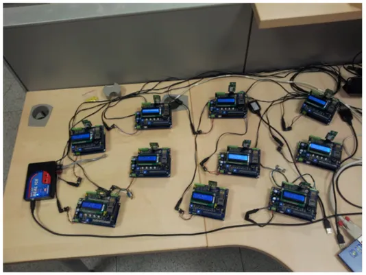
6 Experimental Results 58 6.1 Testbed . . . 58
6.2 Results . . . 61
6.2.1 No aperiodic, no sleep budget . . . 62
6.2.2 No aperiodic, sleep budget . . . 64
6.2.3 With aperiodic, no sleep budget . . . 66
6.2.4 With aperiodic, sleep budget . . . 70
6.2.5 Summary . . . 72
7 Conclusions 76
Summary
The technological evolution in the last decade made possible the widespread use of the sensor networks in many fields and with it, also the interest has grown due to the possible vaste range of applications. The design of wireless embedded systems for real-time applications requires a careful management of timing and energy requirements. The delay introduced in the network has a significant impact on the system performance and should be closely evaluated together with the ability of the protocol to delivery the data in time, avoiding its expiration.
This work presents an extension of the WBuST real-time protocol for multi-hop wireless networks composed of embedded devices. These devices, usually battery powered, also requires careful managing of the power con-sumption in order to extend the battery life at most. This protocol organizes the network as a cluster tree and provides the routing capabilities to transfer the packets among the devices, guaranteeing the packet delivery within their deadlines. At the end of the document, an extensive analysis of the protocol performance, through experimental tests, are presented.
List of Figures
1.1 Block diagram of a smart sensor device. . . 3
1.2 Classification of the wireless networks based on the covered area and the transmission speed. . . 5
1.3 Networks classification based on the interconnection structure. 6 1.4 Overview of a Real-Time Operating System architecture. . . . 7
1.5 Utility function for all the five different kinds of task. . . 8
2.1 IEEE 802.15.4 Network topologies. . . 11
2.2 IEEE 802.15.4 Superframe structure. . . 13
2.3 Master-Slave protocol functioning in a bus topology. . . 14
2.4 Token Passing protocol with a Round Robin scheduling in a bus topology. . . 15
2.5 TDMA protocol in case of 4 nodes sharing the same channel. . 16
3.1 WBuST single-hop network topology. . . 20
3.2 Parameters describing a stream. . . 21
3.3 Maximum delay a message may experience. . . 22
3.4 WBuST Communication window structure. . . 23
3.5 Example of bandwidth reclaiming mechanism. . . 26
4.1 Example of a WBuST Multi-Hop network topology. . . 29
4.2 Inter-cluster communication between a pair of cluster. . . 30
4.3 Example of a WBuST clustered-tree binary network and the relative traffic schedulation. . . 32
4.4 Incoming and outgoing flows in a tree cluster. . . 35
4.5 WBuST source files dependency diagram. . . 38
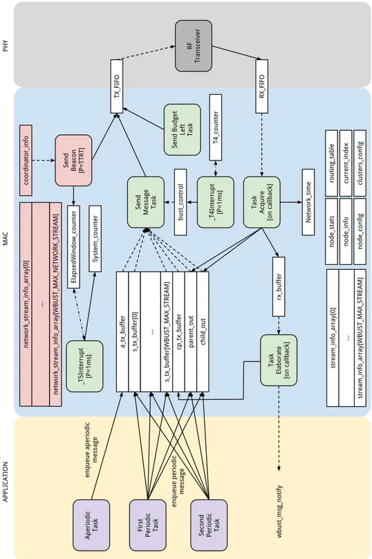
4.6 WBuST Node structure. . . 40
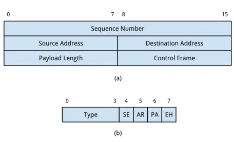
4.7 WBuST Packet header structure. . . 43
4.8 Beacon packet structure. . . 44
LIST OF FIGURES v
4.9 Budget left packet structure. . . 45
4.10 Periodic packet structure. . . 46
5.1 FLEX Light Base board. . . 49
5.2 FLEX Full Base board. . . 50
5.3 FLEX Demo Daughter board. . . 50
5.4 General block diagram of the dsPIC33FJ256MC710 Micro-controller. . . 51
5.5 Easybee module with the CC2420 transceiver. . . 52
5.6 Simplified block diagram of the CC2420 transceiver. . . 54
5.7 Erika Enterprise layered architecture. . . 55
5.8 Development process for OSEK applications. . . 56
6.1 Network topology used to test the WBuST protocol. . . 59
6.2 Set of 10 FLEX boards employed to analyse the WBuST per-formance. . . 60
6.3 Latency with no aperiodic traffic and no sleep budget . . . 62
6.4 ADMR with no aperiodic and no sleep budget . . . 63
6.5 Sleep time with no aperiodic traffic and no sleep budget . . . 64
6.6 Periodic received with no aperiodic traffic and no sleep budget 65 6.7 Latency with no aperiodic traffic and with sleep budget . . . . 65
6.8 ADMR with no aperiodic traffic and with sleep budget . . . . 66
6.9 Sleep time with no aperiodic traffic and with sleep budget . . 67
6.10 Periodic received with no aper. traffic and with sleep budget . 67 6.11 Latency with aperiodic traffic and no sleep budget . . . 68
6.12 ADMR with aperiodic traffic and no sleep budget . . . 69
6.13 Sleep time with aperiodic traffic and no sleep budget . . . 69
6.14 Periodic received with aperiodic traffic and no sleep budget . . 70
6.15 Aperiodic received with aperiodic traffic and no sleep budget . 71 6.16 Latency with aperiodic traffic and sleep budget . . . 71
6.17 ADMR with aperiodic traffic and sleep budget . . . 72
6.18 Sleep time with aperiodic traffic and sleep budget . . . 73
6.19 Periodic received with aperiodic traffic and sleep budget . . . 73
6.20 Aperiodic received with aperiodic traffic and sleep budget . . 74
6.21 ADMR comparison among the four scenarios . . . 74
6.22 Estimated saved energy comparison among the four scenarios for C1 . . . 75
Acronyms
WSN Wireless Sensor Network
LR-WPAN Low Rate-Wireless Personal Area Network
FFD Full-Function Device
RFD Reduced-Function Device
ZC Zigbee Coordinator
ZR Zigbee Router
ZED Zigbee End Device
ADC Analog to Digital Converter
TTRT Target Token Rotation Time
TTHT Target Token Holding Time
CSMA Carrier Sense Multiple Access
CSMA\CA Carrier Sense Multiple Access\Collision Avoidance CSMA\CD Carrier Sense Multiple Access\Collision Detection
CCA Clear Channel Assessment
LQI Link Quality Indication
RSSI Received Signal Strength Indicator
BER Bit Error Rate
MCU Micro-Controller Unit
DSC Digital Signal Controller
ISR Interrupt Service Routine
CW Communication Window
BAS Budget Allocation Schemes
PA Proportional Allocation
NPA Normalized Proportional Allocation
LA Local Allocation
MLA Modified Local Allocation
WCAU Worst Case Achievable Utilization
DMR Deadline Miss Ratio
ADMR Average Deadline Miss Ratio
1
Introduction
1.1 Wireless Sensor Networks . . . 1 1.2 Smart Sensors . . . 3 1.3 Network Classifications . . . 4
1.4 Embedded Real-Time Systems . . 6
Nowadays, thanks to the continuously increasing technological evolution in such fields like computer science, electronics and telecommunications, and the miniaturizing capabilities reached by the current production standards, sensors have spread everywhere. Starting from simple tasks like acquiring and elaborating physical signals, they evolved to the point of being able to cooperate among them, building up networks, exchanging data and providing high computational capabilities systems. That is where the definition Smart
sensors comes from.
1.1 Wireless Sensor Networks
A sensor network (Wireless Sensor Network or WSN) is a group of smart sensors connected each other through appropriate interfaces capable of ex-changing control and monitoring information to reach a given objective [1]. Each sensor is commonly a transducer that is tightly bound to the measured system. Each unit could be connected to the others by two main ways: ca-bles or wireless communications. Caca-bles connections are generally used when there are no particular limitations about the power consumed by the devices or the communication infrastructure is partially existing. Besides, this sys-tem enforce the security of the transmitted data since, to be able to read the information exchanged, a physical access to the communications line is required. On the other side this system entails potentially critical issues such
as the difficulty of installation and maintenance in harsh environments, the placement cost of the devices and the correspondent cables, and the difficulty of adding or moving around the sensors due to the intrinsic static nature of the infrastructure.
Due to this latter problems, wireless networks seem to be a much better solution, even if additional issues like signal propagation, interference, noise, security and also legislations have be faced. All these aspects concur to the project design complexity that immediately reflects on the final realization costs. That is why is important to carefully assess the needs that the designed system has to satisfy, in order to provide the best solution minimizing costs, potential problems and anticipate future enhancements.
The main objective of a sensor network is to collect, verify, elaborate and distribute the data gathered by every single sensor in such a way that, after some time, the network, as a whole, got a wide and uniform information on the monitored system. Since generally, every basic unit, does not have big power and computational capability, it is important to reduce unnecessary data transmission or whatever other kind of energy waste at the most.
Even if it is possible to use the algorithms adopted in the ad-hoc wireless networks, usually they are incompatible with the requirements needed by the sensor networks. The main reasons are:
• the number of nodes belonging to a sensor network could be orders of magnitude bigger than those in an ad-hoc network
• spatial density of the sensors could be really high • sensors have tight power budget to observe
• the network topology could vary frequently in time
• sensors could experience failures or malfunctionings and these should not affect the network efficiency
• sensors generally adopt a broadcast communication scheme
The relative small distance among the sensors allows to use multi-hop com-munication strategies to connect sensors within the same network or between neighbouring ones. This permits lower transmission power consumption, im-proving the node energy requirements. This is a fundamental aspect since sensors operate with power sources that generally cannot be replaced or, at least, replaced frequently.
The needs asked by the sensor networks, pushed the industry to the cre-ation of a new infrastructure called Low Rate-Wireless Personal Area Network
CHAPTER 1. INTRODUCTION 3 (LR-WPAN), characterized by small range communications, low energy con-sumption and low transmission speed. The LR-WPANs are easy to install, provide reliable data transfer, are cheap and they maintain a simple and flex-ible protocol. In the last years, companies are getting even more interested to the applications that can be built with the WSN, basically for three rea-sons: the reduction of the costs due the installation as well as the testing and verification phases, the reduction of the number of movable parts (like the connectors) potentially subject to failures and the increment of the sensors density that could provide more accurate data about the industrial processes leading to an improvement of the production quality.
1.2 Smart Sensors
Smart Sensors are much more than simple transducers of physical quantities
in that they have measuring, storage, computing and communication capa-bilities to provide the correct and unbiased representation of the monitored data. The heart of these integrated devices is the microcontroller that coor-dinates in a seamless way all the other modules. A general scheme of a smart sensor is shown in figure 1.1.
Microcontroller Sensor 1 Sensor 2 Signal conditioning Signal conditioning ADC Transceiver Power source External memory
Figure 1.1. Block diagram of a smart sensor device.
The basic blocks a smart sensor consists of are the following:
• one or more sensors to transform the real physical quantity into an analog voltage
• one or more signal conditioning units that appropriately manipulate the analog signal, through operations like amplification, filtering, isolation, etc. to make the sensor output suitable for the next processing stage • an Analog to Digital Converter (ADC) unit that is in charge of
con-verting a continuous analog signal into a sequence of discrete values • an external memory to store data, that could be both permanent
(FLASH) or temporary (RAM)
• a communication interface to exchange data with other devices (cable, infrared, wireless, etc.)
• a microcontroller that is in charge of interfacing with the attached components elaborating the received digital signals, synchronizing and communicating with the other nodes in the network
• a power source (mains, battery, solar panels, etc.) that feeds all the active electronic components
The employment of smart sensors allow to shift the elaboration of the in-formation towards the physical phenomenon, avoiding a central processor in charge of handling all the data coming from the whole monitored envi-ronment. Smart sensors are able to take local decisions, based upon the assessment of the events, preventing the overload of the network as well as the control center of unnecessary, redundant or useless data. The current technological evolution made this kind of devices extremely cheap, expand-ing the base of the potential users. Besides that, thanks to their flexibility, they also allow fast systems design and implementation shortening the time required to reach the market.
1.3 Network Classifications
Networks are usually classified by the maximum range they can cover or, with a more technical view, by the interconnection structure between the nodes. The first classification, shown in figure 1.2, identifies networks by their reach. Generally the range covered by a network is proportional to the maximum bandwidth the network itself can sustain and inversely proportional to the power consumption.
Starting from the smallest one, we have the Body Area Network (BAN), the
Personal Area Network (PAN), the Local Area Network (LAN), the Metropoli-tan Area Network (MAN) and at last the Wide Area Network (WAN). In the
CHAPTER 1. INTRODUCTION 5
BAN WPAN WLAN WMAN WAN
Range 1m 10m 500m 30km Mobile WIMAX 802.20 802.22 Fixed WIMAX 805.16a/d/e/m Bluetooth (802.15.1) Zigbee (802.15.4) Wi-Fi 802.11b/a/g/n Speed 250kbps 1Mbps 54Mbps 70Mbps
Figure 1.2. Classification of the wireless networks based on the covered area and the
trans-mission speed.
Embedded System field, the first two kinds of networks are the most signi-ficative. A (Wireless) PAN has a quite small range and it is used to inter-connect devices around an individual’s person workspace. The most famous standards for these networks are Bluetooth and Infrared Data Association (IrDA). A BAN, also called wearable network, covers an extremely small range, around as big as a human body volume and it is extensively used for health monitoring systems. These kind of networks allow, for instance, to attach several sensors, detecting different medical parameters, to the human body and periodically communicate them to a base station in charge of their elaboration to provide a complete overview of the patient conditions to the personnel.
For what concerns the network topologies, there exist several models, the most important ones are shown in figure 1.3.
The first three topologies, ring, mesh and bus don’t strictly need a node that coordinates all the others to allow the communications. All the nodes can, in a distributed way, exchange messages with the others, possibly following alternative paths and increasing the robustness of the network. These kind of networks are scalable and cost-effective, even if the bus topology has a limit on the maximum number of nodes that can be attached, after which the shared medium becomes too crowded and the efficiency starts to drop.
Then we have the tree and the star topologies, characterized by an hi-erarchical organization. The tree topology has a root node that acts as the main coordinator and all the other nodes. Actually the star topology can be seen as a tree with only two hierarchical levels. In these kinds of network, the communications are managed by one or more nodes called coordinators,
RING MESH
STAR TREE
BUS
CLUSTERED
Figure 1.3. Networks classification based on the interconnection structure.
in charge of synchronizing the transmission to and from all the other nodes. There exist also hybrid approaches like the clustered networks, in which, nodes are splitted and grouped together forming clusters. Inside each cluster the nodes are connected together with a mesh or a star for instance, and then the clusters are connected each other through a hierarchical structure. Every cluster has an elected coordinator node, representing the access point to the subnetwork, that is connected with the coordinators of the other clusters to exchange inter-cluster traffic. This kind of approach drastically reduces the number of connections required with respect to a mesh topology without worsening too much the latency between the nodes and allowing a better organization of the network.
1.4 Embedded Real-Time Systems
An Embedded Real-Time system is a special-purpose computing system ded-icated to handle a particular task within a larger system for which, the func-tional correctness doesn’t depend only on the validity of the results but also on the time taken to produce those results [2]. Since the embedded sys-tems are dedicated to specific tasks, completely known in the design phase, the hardware can be tailored to satisfy the required needs reducing the size and the costs to the minimum, enforcing both reliability and performance. The platforms upon which an embedded system may be build are various, depending on the required computing capabilities, complexity and power consumption. Microcontrollers range from the most basic components like the Programmable Logic Controller (PLC), to more complex ones like ARM,
CHAPTER 1. INTRODUCTION 7 PIC and Atmel architectures. They can be equipped with internal permanent memory storage (EEPROM memory), oscillators, timers, Analog-to-Digital and Digital-to-Analog converters, Pulse-Width Modulation (PWM) genera-tors, built-in USB and Ethernet interfaces. Nowadays embedded systems are everywhere: telecommunication, automotive industry, medical equipment, consumer electronics, household appliances, transportation and military are just a few examples of fields in which these systems are deeply rooted. Be-cause of that, these systems have to face events that happens in the real world and they have to handle them with an appropriate reaction time. Therefore, quite often, embedded systems are real-time systems as well.
A real-time system, as the name suggests, is a system that has to provide not only correct results, but also within a given time constraint and the speed at which the system time flows has to be the same as the speed of the time in the real world. In this way a real-time system can promptly react to events happening in the physical world. On these kind of systems, a particular class of operating systems are used, the Real-Time Operating Systems (RTOS). A general overview of a RTOS is shown in figure 1.4. A RTOS doesn’t
Figure 1.4. Overview of a Real-Time Operating System architecture.
necessarily be fast, but it should guarantee that a task execution ends within a given predetermined time, called deadline. Indeed, the most important aspect for a RTOS is the predictability. To guarantee in advance whether a task will end within its deadline or not, a feasibility test has to be performed. The feasibility test tells if a set of tasks can be scheduled in such a way that all of them will respect their own deadlines.
There are basically five kinds of tasks that can be handled by a RTOS (listed basing on the increasing criticality): non real-time, soft real-time, firm real-time, on-time and hard real-time [3]. To evaluate the performance of a
scheduling algorithm on a task set, an utility function is defined for all the five classes of tasks (fig. 1.5). Each utility function reflects the value that a
t c(t) t c(t) d t c(t) d t c(t) d
-∞
NON REAL-TIMEFIRM REAL-TIME HARD REAL-TIME
SOFT REAL-TIME
t c(t)
d ON-TIME
Figure 1.5. Utility function for all the five different kinds of task. task has depending on its completion time:
• Non real-time tasks: they don’t have any time constraints, served with a best-effort policy, their value is proportional to their importance and independent of the completion time.
• Soft real-time tasks: they have a deadline, and their value is constant till the deadline, after which it starts to decrease. It means that they can tolerate a deadline miss, up to a given amount of time.
• Firm real-time tasks: they have a deadline, after which the execution of the tasks becomes useless but not harmful and they can actually be discarded.
CHAPTER 1. INTRODUCTION 9 • On-Time real-time tasks: they have a deadline and their value is high only if the task is completed around the deadline, not too early and not too late.
• Hard real-time tasks: they have a rigid deadline to abide by. Missing the deadline might cause unpredictable catastrophic consequences on the whole system, in fact invalidating it.
Very often, real-time systems need to exchange data among them. During data communications between these systems, three kinds of error could occur: • Information error: when the system is not able to interpret the data
or the data is interpreted in a wrong way
• Timing error: when the system is not able to provide data before its expiration
• Transmission error: when the data is corrupted along the way through the communication channel
The last kind of error is most likely to occur with wireless communications since the medium is shared and noise as well as interferences could impair the signal. Therefore, two Quality of Service (QoS) parameters are defined to control the network behaviour: the Deadline for delivery (DL) that states the latest time at which the receiver must receive the information being sent and the Probability of correct Delivery within Deadline (PDL), strictly correlated to the channel quality, that controls how reliable the transfer must be [4].
In the non real-time applications the correctness of the transmitted data is more important than its timing, indeed algorithms such as error detection and correction or packets retransmission are used to ensure the data integrity despite the potential delays they could introduce.
2
Communication Protocols
for Sensor Networks
2.1 IEEE 802.15.4 LR-WPAN . . . 10
2.1.1 Physical layer . . . 12
2.1.2 Medium Access Control . . 13
2.2 Medium Access Control . . . 14
2.2.1 Master-Slave . . . 14
2.2.2 Token Passing . . . 15
2.2.3 TDMA . . . 15
2.2.4 FDMA . . . 16
2.2.5 CSMA . . . 17 2.2.6 Real-time system protocols 18
While in the general-purpose systems, all the seven layers of the Open Sys-tems Interconnection (OSI) model are usually implemented, in the real-time systems field this becomes unfeasible due to the inevitable and unacceptable delay that all these layers would introduce. The main goal is to reduce at most the number of layers and the processing time required for each of them in order to have fast communication stack percolations. Therefore, for real-time sensor networks, only three layers have been kept: Application, Data
Link and Physical. In case additional layers are required by an application,
they could be partially added and integrated with the ones already present.
2.1 IEEE 802.15.4 LR-WPAN
The main features of the IEEE 802.15.4 standard are network flexibility, low cost, very low power consumption, and low data rate in an adhoc self-organizing network among inexpensive fixed, portable and moving devices.
CHAPTER 2. COMM. PROTOCOLS FOR SENSOR NETWORKS 11 It is developed for applications with relaxed throughput requirements which cannot handle the power consumption of heavy protocol stacks [5].
The two basic kinds of devices defined in this standard are the
Full-Function Device (FFD) and the Reduced-Full-Function Device (RFD). The first
kind, is a device that has the full functionalities at the MAC layer, while the second has a reduced set of functionalities. This allow an RFD to save power thanks to the less computational capabilities required. ZigBee, a protocol for wireless low-power communications based on the IEEE 802.15.4, defines the same three kinds of devices as: ZigBee Coordinator (ZC) in place of PAN Coordinator, ZigBee Router (ZR) in place of Full-Function Device and
ZigBee End Device (ZED) in place of Reduced-Function Device.
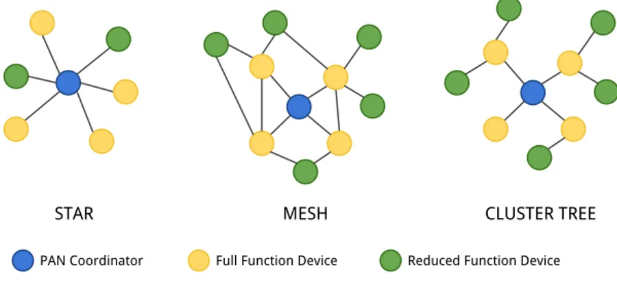
An LR-WPAN has to contain at least one Full-Function Device operating as the PAN coordinator, that is a node in charge of managing the WPAN network. These devices can be combined together forming different network topologies, as the ones shown in figure 2.1.
STAR MESH CLUSTER TREE
PAN Coordinator Full Function Device Reduced Function Device
Figure 2.1. IEEE 802.15.4 Network topologies.
The star topology relies on a central PAN coordinator device, to which the others node can establish connections. The PAN Coordinator is in charge of accepting the other devices join or leave requests and handling as well as routing the communication between the devices. The PAN coordinator may be mains powered while the devices will most likely be battery powered. Every FFD, when turned on for the first time, may create its own network, choosing a PAN identifier not used by other coordinators in its range.
The mesh or peer-to-peer topology, requires just one PAN Coordinator as in the previous case, but the other nodes are free to communicate among them, provided that they are within each other range. This kind of network is much more robust than the previous one since the devices can use distributed algorithms to self-organize themselves and self-heal the network in case of
failures. Moreover, messages sent by nodes, can benefit of multipath routing, increasing the delivery reliability.
At last, the cluster-tree topology adds the concept of clusters to the net-work. The first FFD device that becomes a PAN Coordinator, also creates a cluster, becoming the Cluster Head (CLH) of it. The subsequent devices, may ask to join that cluster and, if the coordinator allows them, they become its childs. The newly joined devices start to send beacons that could be re-ceived by other interested devices. After some time, the PAN Coordinator may instruct a device to become the Cluster head of another cluster, con-nected to the first one. In this way it is possible to increase the reach of the network, with the unavoidable drawback of increasing the message latency.
The structure of a LR-WPAN device is composed of a PHY layer, which contains the radio frequency (RF) transceiver along with its low-level control mechanism, and a MAC sublayer that provides access to the physical channel for all types of transfer. Above them, there are the layers that provide the desired function of the device.
2.1 Physical layer
The PHY layer offers three data transmission rates based on the frequency band used. Low frequencies allow longer reach with lower propagation losses at a cost of reduced transmission speed, while high frequency is used for faster low-ranged communications. The details about the available frequencies and the correspondent modulation formats are shown in table 2.1.
Frequency band Chip rate Modulation Bit rate Symbol rate Symbols Channels
[Mhz] [kchips/s] [kbit/s] [ksymbols/s]
868-868.6 300 BPSK 20 20 Binary 1
902-928 600 BPSK 40 40 Binary 10
2400-2483.5 2000 O-QPSK 250 62.5 16-ary Orthogonal 16
Table 2.1. IEEE 802.15.4 PHY layer frequency bands and transmission speeds.
The receiver sensitivities of -85dBm at 2.4Ghz and -92dBm at 868/915Mhz, together with the transmit power, determine the maximum achievable range. The PHY, in addition to generating and modulating the carrier and (de)-coding data, performs also three evaluations during its functioning: Receiver Energy Detection (ED), Link Quality Indication (LQI) and Clear Channel Assessment (CCA). These parameters are used to monitor the quality of the communications and to take actions whenever it drops under a fixed threshold.
CHAPTER 2. COMM. PROTOCOLS FOR SENSOR NETWORKS 13 2.1 Medium Access Control
IEEE 802.15.4 provides two ways to access the medium, one called Beacon
Enabled and the other one Non Beacon Enabled. The Beacon Enabled mode
uses a periodic packet called superframe that allow the nodes to synchronize with the coordinator. In this way the coordinator can schedule the trans-mission periods of all the nodes in its network. Instead, in the Non Beacon
Enabled mode, the access to the channel is completely unregulated and
there-fore totally asynchronous. Independently on which of the two modes is being used, all the nodes have to register to the coordinator, with a procedure called Association. It is the job of the coordinator to keep a list of all the associated devices, to send the periodic beacon (if required), and to exchange packets with the neighboring nodes.
In the Beacon Enabled mode, the communication window contained be-tween the transmission of two consecutive beacons, can be divided into 3 parts (fig. 2.2): a Contention Access Period (CAP) during which the chan-nel is accesses with the CSMA/CA technique and used to exchange control information, a Contention Free Period (CFP) in which each node transmits only during the time slot it has been assigned to by the coordinator (called
Guaranteed Time Slot or GTS) and, at last, an Inactive period used to save
power, for instance turning off the radio transceiver [7].
Contention Access Period GTS 1 GTS 2 GTS 3 Beacon
ms
0 1 2 3 4 5 6 7 8 9 10 11 12 13 14 15
Inactive Contention Free Period
Figure 2.2. IEEE 802.15.4 Superframe structure.
During the Contention Access Period, the devices use a CSMA/CA protocol, while during the Contention Free Period they access the channel with a Time-Division strategy. Each device, during its GTS, should guarantee that its transmission stops before the beginning of another device GTS. A coordinator can allocate up to 7 GTS for each superframe and each GTS can occupy more than one time slot. In any case, the superframe has to contain a minimum CAP. Another solution uses the whole superframe as a CAP, becoming in fact a CSMA protocol.
2.2 Medium Access Control
The Medium Access Control (MAC) layer of a protocol, manages how a device accesses the transmission medium to send its data. Two big families of MAC protocol can be distinguished:
• Controlled Access: this is a collision-free class of protocols since each node knows when it is allowed to transmit, therefore avoiding collisions with other transmitting nodes. The protocols like Master-Slave, Token-Passing and TDMA belong to this family.
• Uncontrolled Access: this is a class of protocols in which transmis-sions take place as soon as the node has some data to transmit. This imply no cost at all to organize the devices, but with the probability that a transmission could overlap with someone else. In case, the de-vices should detect the collision and provide mechanisms to retransmit the packets. Protocols like CSMA, CSMA/CA, CSMA/CD belong to this family.
2.2 Master-Slave
Master-Slave protocols define a single node acting as a coordinator, called
master, while all the other nodes are called slave. All the slaves, prior to
transmit, have to wait to be authorized by the master. The master could apply any scheduling algorithm without the need of synchronizing the nodes, but with two drawbacks: the need of sending a control message for every
slave activation and the existence of a single point of failure (fig. 2.3).
Master
Slave 1 Slave 2 Slave N Shared bus
CHAPTER 2. COMM. PROTOCOLS FOR SENSOR NETWORKS 15 2.2 Token Passing
In the Token Passing protocols, the access to the medium is allowed only when a node has a special packet called token. This packet is exchanged among the nodes with an order dependent on the utilized scheduling algorithm. The most common scheduling strategy used is called Round Robin. With this scheduling, the devices are enabled to transmit in a circular way (fig. 2.4). The advantage is that collisions are eliminated, and that the channel band-width can be fully utilized without idle time when demand is heavy. The disadvantage is that even when demand is light, a station having data to transmit must wait for the token, increasing latency.
Node 1
Node N Node 4 Node 3
Shared bus Node 2
Figure 2.4. Token Passing protocol with a Round Robin scheduling in a bus topology. Few parameters are introduced when Token Passing protocols are used:
• Target Token Rotation Time (TTRT): is the time needed to per-form a round trip along the ring
• Real Token Rotation Time (RTRT): is the time effectively taken by the token to percolate the ring the last time
• Token Holding Time (THT): is the time span during which the node owns the token
This protocol should also provide mechanisms to recover the token in case it is lost, otherwise the whole network would result as blocked. When the Token Passing protocols are used in real-time systems, it is necessary to bound the TTRT to guarantee that every node has a transmission window suitable with their transmission deadlines [8].
2.2 TDMA
With Time Division Multiple Access (TDMA), the data stream is divided into frames and, in turn, the frames are divided into time slots. Each devices
is assigned with one or more of these time slots in such a way that the com-munication does not overlap. Each time slot is separated from the next by a guard interval, necessary to keep into account small synchronization error between the devices (fig. 2.5). TDMA allows multiple devices to share the same transmission medium, like a frequency channel for instance, guarantee-ing collision-free communications. The drawback is that a device has a fixed available bandwidth, even in case it has a lot of data to send and the other devices are in idle. For this reason, a Dynamic TDMA has been designed providing on demand assignment of the time slots depending on the device traffic load. Node 1 Node 2 Node 3 Node 4 Frame 1 2 3 4
Time slot Guard interval
Figure 2.5. TDMA protocol in case of 4 nodes sharing the same channel.
2.2 FDMA
The Frequency Division Multiple Access (FDMA) is similar to the TDMA approach, but instead of dividing the time, it partitions the frequencies. This scheme is immune to the timing synchronizations required for the TDMA but, unless a device is equipped with a full-duplex transceiver, it cannot receive on a frequency and simultaneously transmit on another. A disadvantage that this kind of protocol has is the crosstalk between adjacent frequency that could impair the communication. In wireless sensor networks, in case of cluster-tree topology, FDMA can be used to assign each cluster a frequency in such a way that local cluster communications can take place at the same time, while for inter-cluster communications the coordinators periodically switch frequency to exchange traffic with the neighboring coordinator devices. FDMA and TDMA can also be combined together to obtain a full partitions
CHAPTER 2. COMM. PROTOCOLS FOR SENSOR NETWORKS 17 of both frequencies and time, increasing the number of available slots as well as the number of supported devices.
2.2 CSMA
The Carrier Sense Multiple Access (CSMA) is a probabilistic medium access control in which a device is able to detect if there is another communication ongoing on the same transmission medium. This is achieved by detecting both the carrier wave and the presence of an encoded signal of some other devices. There exist two versions of this protocol, one is the CSMA with Collision Detection (CSMA/CD), while the other is CSMA with Collision Avoidance (CSMA/CA).
CSMA/CD sends the data as soon as it is ready, detecting later if a collision happened and, in case, stopping immediately the current transmis-sion. In this way the channel is freed just whenever a collision is detected, shortening the time required before another attempt to send. In wireless networks, the Collision Detection approach is not feasible due mainly to the hidden node problem. The other approach, CSMA/CA, is more cautious than the first one in that, before transmitting, it tries to detect an ongoing transmission. In case a node is already transmitting, it simply delays the communication by a random time interval called backoff time, decreasing the probability of collision.
CSMA/CA protocols can also be further subdivided into Non Priority
CSMA/CA and Priority CSMA/CA. As the names suggest, the first version
treats all the packets in the same way, while the second one differentiates them using different rules to distinguish different classes of packets. In real-time networks, of course the priority could be based on the deadline that a packet or a stream of packets have. The policies adopted to distinguish among different priorities are based on:
• inter-frame time differentiation: higher priority packets have a lower inter-frame time, that is the time a packet has to wait, and during which the channel has to remain free, before starting to transmit. • outgoing queue differentiation: each node has as many outgoing
queues as the number of priority classes. Each packet ready to be sent is put in the correspondent queue and waits to be transmitted. The node serves the queues starting from the one with the highest priority and going down till it finds one that is not empty and then sends the first packet of that queue.
inversely proportional to the priority. This allow higher priority packets to wait less in case the channel is already busy when the node transmits. 2.2 Real-time system protocols
MAC protocols for wireless real-time networks have been mainly designed to guarantee an high throughput keeping into account both the bandwidth required and the power consumption, but generally not considering the real-time requirements or the jitter control. Those protocols that keep into ac-count also these factors can be classified following two different systems. The first classification, presented in [9], divides the protocols in synchronous
scheme and asynchronous scheme. The synchronous protocols are those that
require some sort of synchronization among the nodes of the network such as Cluster TDMA [11], Cluster Token, Implicit Earliest Deadline First
(I-EDF) [12], Robust Implicit EDF (RI-(I-EDF) [14], TDMA-Based MAC (TB-MAC) [13] and WBuST [18].
The protocols using a synchronous scheme generally implements a Time Division Multiplex approach subdividing the time into slots assigned to each nodes. This implies the presence of a coordinator node to synchronize all the other devices in the network and the possibility of wasting bandwidth in case a node doesn’t use the whole reserved time slot due to less traffic to transmit or an hardware/software failure.
The asynchronous scheme protocols, usually based on Black-Burst (a broadcast protocol that addresses hidden node and reliability problems in multi-hop vehicular networks) [15] and added with a real-time functionalities, require a fully connected networks and are not easy to extend to multi-hop environments.
Another classification proposed in [10] divides the protocols into three cat-egories: scheduling based, contention based and scheduling/contention based. The first class access the medium in a TDMA manner, since each node ex-actly knows when it is allowed to transmit. In case a node doesn’t have data to transmit or it is less than expected, it could give the amount of time saved to the next node waiting to transmit. The contention based approach, in-stead, is based on the CSMA with Collision Avoidance scheme. They are less performant than the scheduling protocols since the probability of a collision can be reduced but not eliminated. The last category is a mix between the first two. WBuST can be classified as a scheduling/contention based protocol since its time frame is partitioned in a contention period used to exchange control information and a scheduling period used to transmit the node traffic.
3
WBuST Protocol
3.1 Network model . . . 20 3.1.1 Communication Window Structure . . . 22 3.1.2 Protocol properties . . . 23 3.2 Budget Allocation Schemes . . . . 24 3.3 Bandwidth reclaiming . . . 25 3.3.1 Non real-time traffic . . . . 26The Wireless Budget Sharing Token (WBuST) protocol is a MAC layer protocol designed for real-time wireless networks of embedded devices [18]. WBuST can handle real-time and best-effort traffic while applying power saving strategies to guarantee the maximum device lifetimes. The are four main sources of energy waste that can be identified at the MAC level:
• Collision: every time a packet experience a collision and became cor-rupted, it has to be sent again, wasting power
• Overhearing: energy consumption due to listening to the channel and receiving packets addressed to other nodes
• Control overhead: energy consumed by exchanging control packets • Idle listening: energy consumed in receiving mode while waiting for
packets
Contention-based protocols like CSMA/CA are mainly subject to collisions and idle listening issues, while scheduling-based protocols are mainly affected by control overhead. WBuST is an hybrid approach that mitigates both prob-lems, providing an efficient power saving mechanism while still guaranteeing
the real-time stream packet deadlines. WBuST has been designed to operate in both single-hop and multi-hop networks. In this chapter the main con-cepts of the basic single-hop version are introduced, while in the next chapter the extension for multi-hop support is presented.
3.1 Network model
The WBuST protocol is an implementation of the BuST protocol [19] for wireless environments. It belongs to the category of token-passing protocols and it has been introduced to improve the performance of the timed-token protocols like FDDI and FDDI-M in cabled networks [20]. In WBuST, the time slot in which a node is allowed to transmit is shared between the syn-chronous traffic (real-time) and the asynsyn-chronous traffic (non real-time).
A WBuST network is composed of a set of nodes. In every network there is one coordinator node and one or more normal nodes (fig. 3.1). The coordinator is in charge of scheduling the streams transmission, managing the network and synchronizing the nodes together sending periodic beacon messages. Coordinator Node Normal Node N1 N2 N3 N4 N5 N6
Figure 3.1. WBuST single-hop network topology.
Each node i has one or more synchronous message streams Si associated to
it which are described by three parameters (fig. 3.2):
• Ci, the maximum amount of time required to transmit one message of
the stream
• Ti, the interarrival time between two consecutive stream messages
• Di, the relative deadline associated to the stream Si, that is, the
max-imum amount of time that can elapse between a message arrival and the completion of its transmission
CHAPTER 3. WBUST PROTOCOL 21 Stream i, Msg j Stream i, Msg j+1 Ci Ti Di time
Figure 3.2. Parameters describing a stream.
At this point we can define the concept of channel utilization of a stream Si,
that is
Ui =
Ci
min(Ti, Di)
while the total channel utilization is given by the sum of all the stream utilizations U = n ∑ i=1 Ui
where n is the number of streams in the network. Let’s define now few more parameters of the protocol:
• τ is the time needed to transmit the token between nodes, included the overhead introduced by the protocol
• Tb is the beacon period which defines the dimension of each
Communi-cation Window
• TBT is the greatest value of Tb that guarantees the correct operation of
WBuST
The parameter TBT has the same meaning as the Target Token Rotation Time
(T T RT ) for the timed token protocols. To guarantee the correct functioning of the protocol, TBT has to be not greater than the minimum relative deadline
Dmin = mini(Di). This is a necessary and sufficient condition to guarantee
at least one packet transmission for each node i, between the time tr
i a new
message in Si is produced for transmission and its absolute deadline di =
tri+ Di. An example showing the maximum delay a message may experience,
is shown in figure 3.3.
The maximum delay between tr
3 a new message is ready in the stream S3 and
the end of the budget B3in the next CW. The delay is equal to Tb ≤ TBT and
has to be no greater than D3. Given Dmin = D3 and Tb = TBT, the condition
that guarantees at least one packet transmission becomes: tr
3+ Tb ≤ tr3+ D3.
A message experiences the worst-case transmission delay when it is produced just after the end of the budget assigned to its node. For any choice of the
B1 BC B2 B3 Bn-1 Bn BS BC B1 B2 B3 Bn-1 Bn BS Time t3 r t3 r Tb + ≤D3 Tb Maximum delay
Figure 3.3. Maximum delay a message may experience.
protocol parameters, two constraints have always to be satisfied in order to allow a correct communication among the nodes:
• Protocol constraint: the total bandwidth allocated to the nodes must be less than the available network bandwidth, formally written as n ∑ i=1 Bi TBT ≤ 1 − τ TBT
• Deadline constraint: if si,j is the time at which the transmission
of the j-th message in stream Si is completed, the deadline constraint
requires that for i = 1, ..., n and j = 1, 2, ...
si,j ≤ ti,j + Di
where ti,j is the message arrival time and Di is its relative deadline.
It’s worth to notice that in the previous two formulas, while ti,j and Di
are defined by the application, si,j depends on the synchronous bandwidth
allocation and on the TBT value.
3.1 Communication Window Structure
WBuST assigns, to each stream Si, a budget Bi for real-time traffic
trans-mission. From now on we will consider only nodes with one stream, since if a node has more than one stream, we can put together the budgets and consider them as a one big stream. Whenever a node receives the token, it is allowed to transmit up to an amount of time equal to Bi. The asynchronous
traffic can be sent by a node, every time it holds the token and if there is no real-time traffic to transmit.
The TBT is chosen as the smaller Diamong all the streams in the networks.
After the TBT is set, the coordinator computes, for each stream, the relative
CHAPTER 3. WBUST PROTOCOL 23
B1
BC B2 B3 B4 BS
CWk-1 CWk CWk+1
Beacon Guard Intervals
Figure 3.4. WBuST Communication window structure.
periodic intervals called Communication Window (CW), whose structure is illustrated in figure 3.4.
Each CW starts with a special packet sent by the coordinator node called
beacon. The beacon is used to communicate the CW length, synchronize the
node and communicate the CW schedule. Each CW is divided into several kind of slots:
• BC is the contention slot and it immediately follows the beacon. It is
accessed with the CMSA/CA scheme and it is used to exchange control information with the coordinator like joining or leaving the network, reserving slots, etc.
• Bi is the contention-free slot reserved for the node i. In this period,
node i can transmit its synchronous/asynchronous messages.
• BS is the slot collecting all the unused time in the CW and exploited
to put in sleep mode all the nodes to save energy.
Each node has a timer used to count the elapsed time since the beacon re-ception with a resolution of 1ms. Each time slot is separated from the next one by a guard interval, necessary to tolerate the small but unavoidable node synchronization misalignments due to both the limited timer resolution and the not perfectly constant transmission delays.
The contention period can also be removed if the network topology is static and no node joins/departures are expected.
3.1 Protocol properties
The properties that the WBuST protocol exhibits, holds when the constraints are satisfied. There are two properties that bound the maximum delay for a
message, called W Ci, in case of real-time streams only and real-time streams
together with asynchronous traffic.
Maximum delay with real-time streams only. Under the WBuST pro-tocol, if Ti ≥ TBT and the network traffic is only generated by real-time
streams, for i = 1, ..., n: W Ci = ⌈ Ci Bi ⌉ (TBT − Bi) + Ci
Maximum delay with both real-time and asynchronous streams. Under the WBuST protocol, if Ti ≥ TBT and the network traffic is generated
by real-time and best-effort streams, for i = 1, ..., n:
W Ci = ⌈ Ci Bi ⌉ TBT
Since WBuST uses the same channel access strategy of the BuST protocol, the proof of these two properties can be found in [19].
3.2 Budget Allocation Schemes
In order to assign to each stream a budget for transmission, several allocation schemes can be used. The schemes for the timed-token protocols, as in [21] are classified as global or local, depending on the quantity of information they need to provide the scheduling. Local information can be, for instance, the stream set assigned to a node, while a global information is the number of nodes in the network.
Another classification proposed in [24], divides the allocation schemes among the TBT-partitioning and the Ci-partitioning ones. The class of the
TBT-partitioning schemes, computes the stream budget as a fraction of the
maximum value of the beacon period (TBT). The allocation schemes
belong-ing to this category are the Proportional Allocation (PA) and the Normalized
Proportional Allocation (NPA) and are shown in table 3.1. The value α
rep-resents the bandwidth wasted due to the protocol overhead and is calculated as α = τ TBT while βmin = min i Ti TBT
The Ci-partitioning schemes, instead, assign the stream budget as a fraction
CHAPTER 3. WBUST PROTOCOL 25
Scheme Allocation rule U* Schedulability test
PA Bi= Ui(TBT − τ) 1− 3α 2(1− α) U ≤ βmin (1− α) ⌈ βmin 1−α ⌉ − α 1− α NPA Bi= Ui U (TBT− τ) ⌊βmin⌋ ⌊βmin+ 1⌋(1− α) Ti≥ TBT (⌈ 1 1−1−αU ⌉ − 1 )
Table 3.1.TBT-partitioning schemes.
Scheme Allocation rule U* Schedulability test
LA Bi= ⌊ Ci Ti TBT − 1 ⌋ ⌊βmin⌋ ⌊βmin+ 1⌋(1− α) U ≤ ⌊βmin⌋ ⌊βmin+ 1⌋(1− α) MLA Bi= ⌊Ci Ti TBT ⌋ ⌊βmin⌋ ⌊βmin+ 1⌋(1− α) U ≤ ⌊βmin⌋ ⌊βmin+ 1⌋(1− α)
Table 3.2.Ci-partitioning schemes.
the Local Allocation (LA) and the Modified Local Allocation (MLA) and are shown in table 3.2.
The parameter U∗represents the Worst Case Achievable Utilization (WCAU), that is the maximum network utilization for which every real-time message, if U ≤ U∗, is guaranteed to be sent within the deadline [22, 23]. The value of
U∗, calculated for BuST in [25], is still valid also for WBuST since it employs the same scheduling policies [26, 27]. From now on and for all the streams in the network, we will consider Di = Ti. This does not affect the results since
Ui = min(TCii,Di) and therefore the results are valid also the case Di ≤ Ti,
sim-ply by replacing Ti with Di. The WCAU is widely utilized to guarantee the
schedulability of a stream set when only an estimate of the real-time traffic is available, without knowing the characteristics of every real-time message. It is possible to provide also the maximum transmission time for real-time messages with WBuST protocol. Indeed, for all the budget allocation schemes seen till now, if ∀i = 1, ..., n : Ti ≥ TBT, it holds:
∀i, j : si,j ≤ ti,j +
⌈ Ci Bi ⌉ (∑n r=1 Br+ τ )
3.3 Bandwidth reclaiming
In WBuST, whenever a node has less traffic to transmit than expected and doesn’t use its reserved slot completely, the left budget can be recycled to
increase the transmission time of other nodes. Therefore, when a node saves some budget, the unused budget is added to the budget of the next node. The unused budget collected after the last node transmission is added to the sleep budget. In this way the sum of all the node budgets plus the sleep budget is kept constant and equal to Tb. This means that the saved
budget cannot be used across different CWs, since it is depleted in the same CW in which it has been accumulated. This power saving scheme is called
Remainder Sleep Time and allow a dynamic sleep slot adaptation, depending
on the network utilization. Several ways can be used to communicate to a node that the previous budget finished before its expiration. WBuST uses a special message that is sent by node that has no more traffic to transmit to the node owning the next stream allowed to transmit. The following formula, which proof is shown in [18], gives the worst case transmission time for any message of a stream Si, when the budget recycling mechanism is employed.
For i = 1, ..., n, if Ti ≥ TBT + ∑i j=1Bj, then: W Ci = ⌈ Ci Bi ⌉ (TBT − Bi) + Ci+ i ∑ j=1 Bj
The situation causing the maximum transmission delay is shown in figure 3.5.
B1 BC B2 B3 BS BC Tb+ Bi Tb BC BS B1 B2 B3 BS Tb Tb ∑ i=1 3
Figure 3.5. Example of bandwidth reclaiming mechanism.
Indeed, if at the end of BC all the nodes have no traffic to transmit and if
a massage becomes ready in every node, as soon as the sleep budget starts, the node 3 will experience the maximum delay. This because it has to wait its turn that actually is the last one. It is important to notice that the position in the ordering affects the maximum transmission delay between two consecutive channel accesses. This consideration can be used to order the node/stream slots from the one with a shorter deadline to the one with the longest deadline.
3.3 Non real-time traffic
One of the characteristics of the WBuST protocol is the ability to send both real-time and best-effort traffic. Up to now only the real-time traffic
CHAPTER 3. WBUST PROTOCOL 27 guarantees have been studied, hence the minimum bandwidth for best-effort traffic will be analized now. To study the worst-case service for non real-time traffic we suppose that every node has always best-effort messages to send, therefore having the full channel utilization. The minimum bandwidth that a node can reserve for this kind of traffic depends on the budget allocation scheme used. In [19] is shown that for a node i, the minimum bandwidth
UiBE that can be guaranteed for best-effort traffic is:
• with PA scheme UiBE = Ui
( 1
U + 1−αα − 1
)
• with NPA scheme UiBE = Ui
( 1− α
U − 1
)
The value UBE
i can increase in case the nodes have no real-traffic to
trans-mit. Even if each stream has a guaranteed bandwidth for sending best-effort traffic, it is clear that the allocation is not fair. Indeed, the time reserved for non real-time traffic transmission is proportional to the quantity of real-time traffic of the stream. A way to mitigate this situation is to put a limit, for each stream, on the maximum best-effort traffic that can be sent.
4
Multi-Hop Extension for
WBuST
4.1 Network topology . . . 28 4.2 Inter-cluster communication . . . . 30 4.3 Clustered-tree network . . . 31 4.4 Traffic scheduling . . . 34 4.4.1 Bandwidth constraints . . . 34 4.4.2 Budget Allocation Scheme . 36 4.5 Power saving . . . 36 4.6 Implementation . . . 37 4.7 Node structure . . . 39 4.8 Message definition . . . 42 4.8.1 Beacon message . . . 44 4.8.2 Budget left message . . . . 45 4.8.3 Periodic message . . . 45 4.8.4 Aperiodic message . . . 46In this chapter, the multi-hop extension for WBuST is presented. This exten-sion allows a more structured network as well as permitting communications among devices that are not able to directly communicate due to a limited operative range. The multi-hop capability increases also the available band-width, exploiting different channel frequencies at the same time.
4.1 Network topology
In a multi-hop network, the devices are divided into adjacent groups called
clusters. Each cluster is assigned a different radio channel in such a way that,
the transmissions within adjacent clusters can take place at the same time 28
CHAPTER 4. MULTI-HOP EXTENSION FOR WBUST 29 without interfering with each other. Clusters can be connected among them to form various network topologies allowing a great flexibility and adaptabil-ity to different scenarios.
A WBuST network is composed of n clusters, each named Ci. A node in
the network can assume different roles:
• Normal node: a node that exchanges information with the nodes belonging to the same cluster and can send inter-cluster traffic
• Coordinator node: a node located in the central area of the cluster in charge of synchronizing the nodes within its area and scheduling their transmissions
• Router node: a node located in the central area of the cluster in charge of interacting with other router nodes
Very often, especially in the sensor networks field, the nodes performing coordination functions also perform the routing functions, therefore both functionalities are merged within the same device. In figure 4.1 an example of a clustered-tree structured WBuST network is shown.
Cluster 1 Cluster 2 Cluster 3 Coordinator/Router Node Normal node Infra-cluster link Inter-cluster link
Figure 4.1. Example of a WBuST Multi-Hop network topology.
As we can see from the picture, each cluster can employ its own connection topology: the clusters 1 and 3 are organized in a star topology while the clus-ter 2 uses a mesh topology. The employed topology depends on whether the devices belonging to the same cluster are each other in their radio operational reach or not. If they are, they are able to directly communicate among them, otherwise the coordinator/router node has to act as a bridge between them. Of course, this requires that the coordinator/router node should always be directly reachable from every other node within the cluster.
4.2 Inter-cluster communication
While for the infra-cluster traffic the Communication window is the same as in the single-hop protocol, to allow inter-cluster traffic few slots have to be added at the beginning of every CW. To allow communications between two clusters, few rules have to be added. An inter-cluster communication between two clusters, as for instance those shown in figure 4.2 occurs with the procedure described in the next lines. Once the procedure is defined for the basic case, it can be extended for any kind of cluster topology. Let’s identify the coordinator/router nodes as Ri.
BC1 BC2 BC BS BC1 BC2 BC BS 1 1 2 1 1 Tb Cluster 1 Cluster 2 1
Figure 4.2. Inter-cluster communication between a pair of cluster. The rules allowing a correct communication are:
• The link between the two clusters must be synchronized by a beacon transmitted by one of the two coordinators, defined during the design phase to act as a master. In this example the master is R1, which is in
charge of managing the link
• Both clusters must use the same beacon period Tb
• To allow simultaneous communications within different clusters and avoiding packet collisions, each cluster must use different radio chan-nels. Since the devices are usually equipped with low-cost radio mod-ules, they are supposed to work with an half-duplex transceiver that can use only one frequency at a time and cannot receive and transmit simultaneously
CHAPTER 4. MULTI-HOP EXTENSION FOR WBUST 31 • During the period in which the two routers exchange inter-cluster
traf-fic, the radio channel used is the one of the master
• Each router can transmit both real-time and best-effort traffic using a budget BCi assigned at design time
• Both router budgets must be allocated in the communication windows of both clusters
The communication between the two clusters proceeds as follows:
1. At the beginning of each CW in C1, R2 switches to the C1’s channel
and waits to receive a beacon from R1
2. Once the beacon is received, both routers are synchronized and the communication can start. The slot BC1 is used to transfer traffic from
C1 to C2, while the slot BC2 is used to transfer traffic the other way
around. For the master coordinator, the budgets for inter-cluster com-munication are placed just after the beacon, while for the other routers they are placed in succession
3. At the end of the budget BC2, R2 switches to C2’s channel and sends
its beacon to synchronize the infra-cluster communication that starts with the contention period BC
4. Instead, at the end of BC2, in C1 the contention period starts
immedi-ately since it is not necessary to send another beacon
As can be noticed, the bandwidth lost due to the protocol overhead caused by beacon transmissions, is higher in the non-master cluster. This basic scenario can be extended with n clusters connected in several ways like chain, tree, ring, etc.
4.3 Clustered-tree network
This section presents the implementation of the WBuST protocol for clustered-tree multi-hop networks. This topology has been chosen since it is the most adaptable to the common wireless sensor network scenarios while, at the same time, being able to maintain the latency of the communication among the nodes under a reasonable limit even in case of big networks. In this topology, clusters are hierarchically organized as a tree. The root cluster is in charge of starting the first communication window, while the others, in cascade, will propagate the CWs from the parent to the childs clusters.
C1 C2 C3 C4 C5 C6 C7 1 1 2 2 3 3 BC1 BC2 BC BS BC1 BC2 BC BS 1 1 2 1 1 Tb C1 C2 BC3 BC2 BC4 BC5 BC BS 2 2 C4 BC2 BC4 4 BS 2 2 C5 BC2 BC4 BC5 5 BC BC1 BC2 BC BS 1 3 1 C3 BC3 BC3 BC6 BC7 BC BS 3 3 BC3 BC6 6 C6 BC BS 3 3 BC3 BC6 7 C7 BC7
Figure 4.3. Example of a WBuST clustered-tree binary network and the relative traffic
schedulation. The number on top of the beacons represents the cluster that sends that beacon. The arrows among the slots indicate the direction in which the inter-cluster traffic flows.
CHAPTER 4. MULTI-HOP EXTENSION FOR WBUST 33 To explain the principles of the clustered-tree communications, let’s take for instance the network shown in the first part of figure 4.3.
In this topology, the communication between two clusters are synchronized by the parent cluster. The child clusters should therefore wait the parent beacon on its channel. The number written next to the inter-cluster link represents the cluster that is in charge of managing the communication. The communication scheduling starts from the root cluster and propagates down-wards till it reaches the leaf nodes. The schedule of the communication win-dows for this network are shown in the second part of figure 4.3. At the beginning of each CW of cluster C1, R1 sends its beacon to both R2 and R3
that are listening on its channel. Once the beacon is received, C1, C2 and C3
are synchronized and they can start transmitting their inter-cluster traffic within their own respective slots BC1, BC2 and BC3. After transmitting its
messages in BC2, R2 switches on its channel and transmits the beacon to
coordinate the inter-cluster communication with C4 and C5 (that are
listen-ing on C2’s channel) and successively, its own infra-cluster communication.
This procedure is recursively repeated, starting from the root cluster and for every branch, till the last level of the tree is reached. For each cluster, the infra-cluster communication window, as seen in the previous chapter for the single-hop version of WBuST, is composed by a contention period slot accessed with the CSMA/CA protocol, a series of time slots reserved for the nodes and a possible power saving period used to save energy.
As can be noticed by the schedulation graph, apart the first and second level of the tree, every other cluster experiences a delayed start of its CW as big as the bandwidth used by the parent to communicate, in turn, with its own parent. Moreover, the childs of a cluster, are subject to an additional delay due to the order in which they are served. Indeed C3, before being
able to send data to its parent C1, it has to wait the amount of time needed
by C2 to communicate with the parent. The bandwidth wasted due to the
waiting for the preceding brothers communications is shown in the graph as a dotted slot. In this example, the clusters experiencing this kind of delay are C3, C5 and C7. These periods of inactivity can be used to turn off the
radio module and save power. The implementation of this protocol requires a careful management of the synchronization times in order to limit the nodes clock misalignments as the beacons propagate down in the tree.