Alma Mater Studiorum – Università di Bologna
DOTTORATO DI RICERCA IN
CHIMICA
Ciclo XXVI
Settore Concorsuale di afferenza: 03/D1 Settore Scientifico disciplinare: CHIM08
Computational strategies to include
protein flexibility in Ligand Docking
and Virtual Screening
Presentata da: Dott.ssa Rosa Buonfiglio
Coordinatore Dottorato
Relatore
Prof. Aldo Roda
Prof. Maurizio Recanatini
Correlatore
Dott. Matteo Masetti
Prof. Andrea Cavalli
To my lab mates
“In conclusion, I would like to emphasize my belief that the era of computing chemists, when hundreds if not thousands of chemists will go to the computing machine instead of the laboratory, for increasingly many facets of chemical information, is already at hand.
There is only one obstacle, namely, that someone must pay for the computing time.”
I
TABLE OF CONTENTS
1. INTRODUCTION... 1
1.1 BIOMOLECULAR RECOGNITION MECHANISMS ... 1
1.2 PROTEIN FLEXIBILITY IN DRUG DISCOVERY ... 7
1.3 PROTEIN FLEXIBILITY IN COMPUTER-AIDED DRUG DISCOVERY ... 9
1.4 ENSEMBLE-BASED VIRTUAL SCREENING ... 17
1.5 AIM OF THE WORK ... 20
2. METHODS ... 21
2.1 MOLECULAR MODELING ... 21
2.2 MOLECULAR MECHANICS AND FORCE FIELD (FF)... 21
2.3 GENERATING CONFORMATIONAL ENSEMBLE ... 25
2.3.1 MOLECULAR DYNAMICS ... 25
2.3.2 METROPOLIS-MONTE CARLO METHOD ... 30
2.3.3 ENHANCED SAMPLING METHODS ... 31
2.3.4 ELASTIC NETWORK-NORMAL MODE ANALYSIS ... 34
2.4 ANALYSIS OF MULTIPLE CONFORMATIONS ... 37
2.4.1 CLUSTER ANALYSIS ... 37
2.4.2 DIMENSIONALITY REDUCTION ... 40
2.4.3 NETWORK ANALYSIS ... 42
2.5 LIGAND DOCKING AND SCORING FUNCTIONS... 45
2.5.1 GLIDE: DOCKING AND SCORING FUNCTION ... 48
2.5.2 ICM: DOCKING AND SCORING FUNCTION ... 50
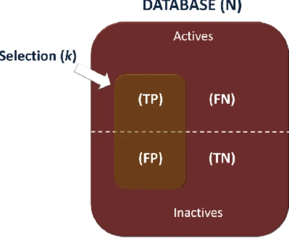
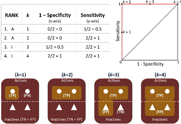
2.6 VALIDATION OF DOCKING RESULTS ... 52
2.6.1 FIGURES OF MERIT ... 52
3. LDHA - CASE STUDY 1 ... 60
3.1 WARBURG EFFECT ... 60
II
3.3 LDHA: STRUCTURAL FEATURES ... 66
3.4 AIM OF THE PROJECT ... 72
3.5 RESULTS AND DISCUSSION ... 72
3.6 SIMULATIONS SETUP AND ANALYSIS PROCEDURES ... 86
3.6.1 THE MINIMAL LDHA MODEL ... 86
3.6.2 hREMD SIMULATION SETUP ... 86
3.6.3 CLUSTER ANALYSIS ... 88
3.6.4 NETWORK ANALYSIS ... 88
3.6.5 RETROSPECTIVE VIRTUAL SCREENING PROTOCOL ... 89
3.5.6 ENSEMBLE-BASED VIRTUAL SCREENING PROTOCOL ... 89
3.5.7 MOLECULAR SIMILARITY SEARCHING ... 91
3.7 CONCLUSIONS ... 91
4. OPIOID RECEPTORS - CASE STUDY 2 ... 93
4.1 OPIOID RECEPTORS... 93
4.2 STRUCTURAL FEATURES ... 96
4.3 OPIOID LIGANDS ... 99
4.4 AIM OF THE PROJECT ... 101
4.5 RESULTS AND DISCUSSION ... 103
4.6 METHODS ... 111
4.6.1 LIGAND DOCKING SETUP ... 111
4.6.2 HOMOLOGY MODELING ... 112
4.6.3 ALiBERO SETUP ... 112
4.7 CONCLUSIONS ... 113
5. CONCLUSIONS AND PERSPECTIVES ... 115
6. ACKNOWLEDGMENT ... 117
1
1. INTRODUCTION
1.1 BIOMOLECULAR RECOGNITION MECHANISMS
Proteins are dynamic structures subject to fluctuations occurring on a wide range of time scales from femtoseconds for ultrafast bond vibrations, to milliseconds and even seconds for large motions, resulting in a broad spectrum of conformations. These motions are at the base of biomolecular recognition, where ligands and receptors move towards complementary conformations to improve the binding affinity and regulate vital biological processes, such as signal transduction, metabolism and catalysis. The mechanisms underlying biomolecular recognition have been investigated extensively, in order to understand these processes and define novel therapies in a drug discovery context. The first explanation for ligand recognition was introduced in 1894 when Emil Fischer proposed the lock-and-key model.1 According to this theory, ligands involved in biological reaction fit perfectly into proteins like a key into a lock, with almost no change in conformation. At that time, when molecular structures were poorly explored, this hypothesis gave an exhaustive and useful visual image of protein functions and was widely used as textbook explanation for biomolecular recognition events. However, the lock-and-key model based on a rigid body collision between ligands and proteins, neglected the emerging role of conformational plasticity supported by X-ray crystallography, NMR spectroscopy and single molecule fluorescence detection.2 On the other side, although underestimating the conformational flexibility, this theory introduced the concept of shape complementarity of the bound components in a macromolecular complex and lasted more than 50 years. Indeed, the lock-and-key model is not completely incompatible with the existence of a protein conformational ensemble. In particular, multiple conformations that interconvert on a time scale faster than binding and dissociation events are indistinguishable from a single structure.3 From a kinetic standpoint, rapidly interconverting species result in the same properties, without changing the observed relaxation kinetics of the system. In this case, for multiple conformations, constants for ligand binding and dissociation (kon and koff, respectively) are defined
2 lock-and-key model may describe properties of single structures or structural ensemble, unless the conformational transitions occur over time scales which are relevant for binding/dissociation processes. The introduction of this model allowed to investigate mechanisms at the base of biomolecular recognition, so as to provide a number of insights to processes spanning from binging events to catalysis. It is clear that this theory did not cover all cases and then, further models were introduced to explain inconsistencies such as noncompetitive inhibition and other relevant discrepancies.5 In the last decades, the concepts of induced fit6 and conformational selection7 emerged to explain the intricate biomolecular recognition mechanisms. In details, the first theory, proposed by Koshland in 1958, was based on the following postulates: ―a) a precise orientation of catalytic groups is required for enzyme action; b) the substrate may cause an appreciable change in the three-dimensional relationship of the amino acids at the active site; and c) the changes in protein structure caused by a substrate will bring the catalytic groups into the proper orientation for reaction, whereas a non-substrate will not‖.6 This theory, generalized to diverse biological mechanisms, pointed out that a fit between macromolecules and ligands occurs only after the changes induced by the substrate itself, likened to the fit of a hand in a glove. It incorporated Fisher‘s concepts of structural complementarity but, at the same time, took into account the enzyme flexibility. However, kinetic studies showed that the induced fit theory failed in describing all possible binding mechanisms.8
In 1965, Monod, Wyman and Changeux proposed the allosteric model assuming that, when an allosteric binding event occurs, a shift of the equilibrium of two(or more) pre-existing conformational states is observed.9 Conformational selection (also referred to as population selection, selected fit and fluctuation fit) is conceptually identical to the original Monod, Wyman and Changeaux model but has been extended to describe a large variety of monomeric non regulated metabolic10-13 or signaling enzymes,14 their intrinsic dynamics, binding mechanisms15 and folding of disordered structures.16 Although this concept was used in the 1980s,17-18 only during last decade it has emerged by the insightful contribution of Nussinov and coworkers as one of the prevalent mechanisms related to biomolecular recognition.16, 19-21 In particular, the description of the energy landscape of proteins by Fraugenfelder, Sligar and Wolynes22 led, in 1999, to the generalized concept of ―conformational selection and population shift‖. The
3 energy landscape is a map of all possible conformations of a molecular entity and their corresponding energy levels on a multidimensional Cartesian coordinate system. Conformations in dynamic equilibrium in the energy landscape are called microstates or conformational substates. It is also referred to as ―folding funnel‖ with many highly unfavorable states that collapse via multiple routes into possibly several favorable folded states.23-25 The populations of these substates follow statistical thermodynamic distributions and the timescale of conformational transitions depends on the height of the energy barriers between substates. In case of low free energy barriers in terms of Boltzmann energy, more than one conformational state can exist in solution. Ligands can bind the most energetically favorable conformations or one of the high energy conformational substates existing in solution. In all cases, this ligand binding causes a population shift, that is a redistribution of the relative populations of conformational substates
pre-existing in solution.
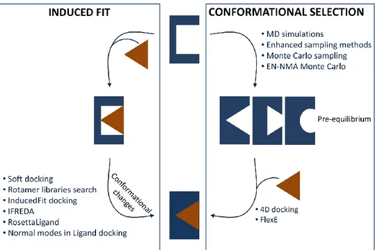
In summary, in both the induced fit and the conformational selection models, macromolecules assume multiple conformations and protein flexibility is considered in binding mechanisms. However, two different scenarios are depicted: one where the conformational ensemble is generated after ligand binding (induced fit) and the other where the conformational transitions pre-exist (conformational selection). In other words, in the former case, the free (unbound) macromolecule is trapped as a single conformation and undergoes conformational transitions when bound, while the opposite situation occurs in the case of conformational selection. Figure 1 shows the free energy landscape of macromolecular structures and binding according to the lock-and-key, induced fit and conformational selection theories. In the first process (Figure 1a), no conformational changes appear after ligand binding and protein exists as the same structure in both the unbound and bound state. In this context, the lock-and-key model can be considered a limiting case of conformational selection where ligand binds to the lowest energy and unique conformation. In Figure 1b, induced fit mechanism is reported: a single protein first binds the ligand and then undergoes conformational changes to optimize the complex, corresponding to multiple substates. In the last case, the free macromolecule pre-exists as conformational ensemble and the ligand binding stabilizes one of them, resulting in a single final substate.
4
Figure 1. The energy landscape view of protein structures and binding. a) Lock-and-key model. b) Induced fit model. c) Conformation selection model. Receptors and ligands are represented in blue and orange, respectively.
Induced fit and conformational selection can be also described through a thermodynamic cycle (see Figure 2 for a simplified scheme). According to this cycle, when the concentration of the higher energy unbound conformation (P2) is
larger than the concentration of P1L, that is the intermediate complex of the
induced fit process, the prevalent biomolecular recognition pathway will be the conformational selection.26 In this latter process, the rate of formation of the final complex P2L depends linearly on the concentration of P2 and nonlinearly on the
total concentration of the protein ([P1 + P2]). On the other side, when the
concentration of the higher energy conformation (P2) is lower than 5%, it is
difficult to distinguish the main biomolecular recognition mechanism between the induced fit and conformational selection.
5
Figure 2. Induced fit and conformational selection in a thermodynamic cycle. P1 and P2
are pre-existing unbound conformations, in agreement with the conformational selection theory. P1L is the intermediate protein-ligand structure which undergoes conformational
changes resulting in the final complex P2L. The capital and lower-case letters for each
equilibrium describe the thermodynamic and kinetic rate constants, respectively. Receptors and ligands are represented in blue and orange.
The mentioned models seem to be antagonistic, as ―all or nothing‖ phenomena. In reality, in many instances, both mechanisms may cooperate in the same processes. For instance, various cases in which conformational selection event is followed by optimization of side chain and backbone interactions based on induced fit mechanisms have been reported.27-28
In this scenario, the original conformational selection model has been extended embracing a repertoire of selection and refinement mechanisms. Induced fit can be thus perceived as a subset of this repertoire contributing to stabilize interactions between bound partners.20 All mechanisms described so far consider a macromolecule as multiple conformations and the second binding partner as a single conformational state corresponding to small and/or rigid ligands, such as small molecules or DNA. On the contrary, in the extended conformational selection model, the ―native states‖ of both binding partners are accounted for as multiple conformations, located at the low-energy regions of the energy landscape. According to this process, binding partners undergo conformational selection and
6 preceding or subsequent adjustment steps, forming the binding trajectory. The mutual encounter modifies the populations of the partner conformations and, thus, the shape of their energy landscape. This mutual condition consisting of step-wise selection and encounter mechanism has been termed as ―interdependent protein dance‖,29
where the conformation of a partner represents the environment (preconditions) for the second molecule and vice versa. The lock-and-key, the induced fit, the original conformational selection and the conformational selection followed by the induced fit are special cases of this extended conformational selection model. It can describe biomolecular recognition processes involving proteins and also the binding mechanism of RNA molecules, as recently reported.30-31
The biomolecular recognition mechanisms can be potentially distinguished by kinetic measurements, based on the dependence of the rate of relaxation to equilibrium, kobs, on the ligand concentration [L].3 For decades, a value of kobs
increasing with [L] has been seen as diagnostic of induced fit, while a value of kobs
decreasing hyperbolically with [L] indicated conformational selection. However, this simple conclusion is only valid under the unrealistic cases in which conformational transitions are rate-limiting in the kinetic mechanism compared to binding and dissociation events. In general, induced fit occurs when values of kobs
increase with [L], but conformational selection is more versatile and is related with values of kobs that can increase, decrease or are independent of [L]. According to
this more adaptable repertoire of kinetic properties, conformational selection is considered always sufficient and often necessary to explain all experimental systems reported in literature so far and then, is fundamental for binding mechanisms. On the other hand, induced fit is never necessary and only sufficient in some biological events. While these two mechanisms can be distinguished by kinetic measurements, direct characterization of sparsely-populated states of proteins in the free and bound forms are experimentally challenging. In fact, unless trapped, such short-lived states are invisible to conventional biophysical techniques like X-ray crystallography and NMR spectroscopy.32-33 Recently, developments in NMR field involving paramagnetic relaxation enhancement (PRE) have led to the detection and exhaustive visualization of these sparsely-populated states, applicable to a wide-range of proteins characterized by transient, short-lived conformational transitions. Moreover, single molecule measurements are emerging tools able to
7 characterize the conformational properties related to protein functions.34 These approaches used to study biomolecular recognition at the single molecule level include the single molecule fluorescence resonance energy transfer (smFRET) and single molecule functional studies. The former reveals the extent and lifetime of conformational motions in catalytic steps and ligand-mediated interconversions between conformations, typically averaged in non-synchronized ensemble measurements.35-36 On the other hand, single molecule functional studies are useful for the direct observation of activity heterogeneities for single and multiple enzymes.37-38 In general, these methods quantify the activity, abundance and lifetime of multiple conformations and transient intermediates in the energy landscape.
The development of the mentioned theories revealed the critical role of protein flexibility for the recognition mechanisms in all biological systems. That being so, protein plasticity has important consequences on drug design and must be considered as fundamental requirement to study biological processes and identify and design small molecule inhibitors.
1.2 PROTEIN FLEXIBILITY IN DRUG DISCOVERY
Protein flexibility is required for biological effects, metabolism, transport and function. For example, residues involved in the catalytic mechanism of enzymes are often flexible, some receptors need to transmit the message of ligand binding from outside the membrane to the inside, channels can exist in an open or close form, etc.39 Protein functions are poorly understood when a single protein structure is under investigation, since typical intrinsic dynamics and wide range of motions are neglected. In other words, using a single protein conformation in a drug design approach to accommodate all ligands corresponds to accept the outdated lock-and-key model of binding.
Conformational changes of side chains within binding sites are essential to identify novel inhibitory compounds. It is known that 8 out of the 20 amino acids can undergo structural rearrangements with a chance of 10-40%, making rigid structures unsuitable for structure-based drug discovery applications.40
8 In a more realistic scenario where multiple conformations pre-exist, design of molecules stabilizing specific structures within the ensemble may improve the probability to succeed in discovering novel active compounds and better understand biomolecular recognition processes. Therefore, proteins can adopt several conformations forming what is known as conformational ensemble. Protein motions are also important in terms of selectivity. Several therapeutic targets belong to families of highly related proteins and then, selectivity is required for pharmacological activity. In particular, binding sites consist of conserved residues located in almost the same positions, as a consequence of binding of the same natural ligands or because these macromolecules carry out reactions with the same chemistry. On the other side, the remaining residues are less homogeneous and promote different types of protein motions. This flexibility bestows a kind of diversity among proteins otherwise similar, to be exploited in the search for selective ligands.39 Also, the understanding of binding mode and affinity based on interaction among compounds, proteins and water molecules, is really important for rational drug design. Free energy that quantifies the preference of a state (free or bound) compared to the others, conveys the affinity of binding events. In the light of these considerations and of the influence of flexibility on drug design, several tools are now available to explore the conformational space and estimate of free energy of binding.
The first attempt to take advantage of protein plasticity has been the use of multiple protein structures derived from NMR studies and X-ray crystallography, considered as the key methods to characterize molecular structures. In many cases, using conformational ensemble improves predictivity of Virtual Screening, but only a limited set of conformations for all existing proteins has been experimentally solved so far. Crystal structures are sometimes heterogeneous due to crystal packing effects, even errors or uncertainties introducing inaccuracies in structures, especially when they are solved at a resolution higher than 1.6Å.41 Another way to generate multiple conformations to be employed in structure-based drug design approaches is the use of computational tools including ligand docking,40 low-frequency normal modes,42 and sampling approaches, such as Molecular Dynamics (MD),43 enhanced methods44 and Monte Carlo simulations.45 They represent a valid alternative to experimental techniques, since they provide an atomistic-level detail to several processes such as protein folding46 or biomolecular
9 recognition,47 and help to define biologically and pharmacologically significant conformations sometimes difficult to characterize with experimental methods. In addition, these techniques allow the identification of additional putative binding sites that may result hidden in the unbound protein structures, shedding light on potential allosteric sites. This scenario points out the importance of protein flexibility in discovering new drugs involved also in allosteric pathways. Ultimately, computational and experimental approaches together seem to be the best combination to study protein fluctuations and interactions.48
Overall, these methods probe both local receptor flexibility in close proximity to the binding site and global flexibility of protein domains, corresponding to side-chain and backbone fluctuations, respectively. In particular, backbone flexibility concerns large-scale domain fluctuations and disordered regions such as flexible loops.49 In the next paragraphs the available computational methods used to probe local and global flexibility are overviewed.
1.3 PROTEIN FLEXIBILITY IN COMPUTER-AIDED DRUG DISCOVERY In consideration of the wide diversity of computational methods employed to study protein flexibility, some kind of classification can be useful. In particular, we can distinguish: i) approaches investigating local and/or global flexibility and ii) protocols that make use of unique or multiple structures. However, an absolute classification cannot be defined and, also, the selection of the most appropriate approach depends on the features of the biological system of interest.
Procedures taking into account single protein structures subject to slight side chain movements are described. The first and easiest way to consider small conformational fluctuations within a protein binding site is the use of implicit methods.50 Many force-field docking algorithms compute the van der Waals forces through the Lennard-Jones potential which increases rapidly to infinity when interatomic distance reduces to zero. It results in large energy penalties when minor steric clashes arise. In other words, potential good binders that do not fit exactly into the rigid binding site, may result in a low rank and bad score. With this method, known as ―soft docking‖, the Lennard-Jones potential is softened through the introduction of a more forgiving potential; thus, minor steric clashes are tolerated and pose orientations including slight overlaps between ligands and
10 proteins are retained, allowing an approximate consideration of protein plasticity. Soft docking is efficient in terms of computational costs, because no additional calculation time is required to evaluate the scoring function and is easily implemented in docking software. However, its main limitation is that it increases the number of false positives and the flexibility is only indirectly taken into account.
Another simple way to include side chain torsions in ligand docking algorithms arises from the reorientation of hydrogen atoms. In particular, rotational sampling of hydrogens and lone pairs of hydrogen-bond donor and acceptor atoms have been included in genetic algorithms, allowing for the promotion of stronger hydrogen bonds.51 Some computational methods accounting for full side chain flexibility are based on an extension of this simple approach, where torsional sampling around single and double bonds are evaluated while bond lengths and angles are kept fixed. These algorithms incorporating side chain mobility use rotamer libraries, introduced for the first time by Leach.52 According to his method, no rotameric states have been assigned to alanine, glycine, and proline. Methionine, lysine, and arginine have been given 21, 51, and 55 rotameric states, while the remaining amino acids range from 3 to 10 rotameric states. Thus, the most energy favorable combination of side chain conformers and ligand orientations is defined. A further approach combines the use of rotamer libraries to generate multiple side chain conformations and an energetic optimization of the docked system, in particular of the side chains in close contact with ligands, so as to strengthen molecular interactions.53 Optimization techniques include simulated annealing, steepest-descent minimization, Monte Carlo (MC) sampling, or other methods.54
A different procedure, that still considers side chain rearrangements, is introduced with the ―InducedFit‖ docking developed by Sherman and coworkers and implemented as a tool of GLIDE docking software, in the Schrödinger suite.55-56 In this case, it accounts for both ligand and protein flexibility and iteratively combine rigid receptor docking with protein structure prediction techniques (GLIDE and PRIME tools).55 By paraphrasing the name, induced fit rearrangements and local movements within the active site upon ligand binding are included in docking protocol. The first step is the ligand docking with GLIDE. During this step, highly flexible side chains can be temporarily removed and converted with alanine residues, so as to reduce steric clashes. For each pose, PRIME tool is used for
11 structure prediction, in order to reorient side chains and accommodate the ligands. Then, ligands and binding site are energy minimized. Finally, a re-docking of each ligand in the low energy protein structure is performed, and small molecules are ranked according to the GLIDE score. A similar algorithm known as IFREDA (ICM-flexible receptor docking algorithm) has been developed by Cavasotto and Abagyan, to define multiple conformations when a single protein structure is available.57 IFREDA generates a set of protein conformations through a flexible ligand docking of known active compounds to a flexible receptor. The resulting conformational ensemble is used for flexible ligand–rigid receptor docking and scoring. Finally, a merging and shrinking procedure allows to condense results of the multiple Virtual Screenings, so as to improve the enrichment factor. With the exception of some few cases, the mentioned techniques probe mainly local receptor flexibility.
An alternative method is RosettaLigand, implemented in the popular software Rosetta, which incorporates full protein backbone and side chain flexibility and considers both ligand ensemble generation and receptor movements during docking steps.58-59 The latest release includes new features, such as docking of multiple ligands simultaneously and redesign of the binding interface during docking.60 However, treating backbone flexibility in docking protocols remains certainly challenging, because a large number of degrees of freedom needs to be considered. Several other methods have been published so far, which consider global flexibility, and also slight side chain movements. They are mainly based on the use of multiple protein structures and are known as ensemble-based methods. Conformations can derive from NMR or crystal structures or computational methods exhaustive in sampling large conformational space and derived from the protein flexibility analysis, as already introduced in the previous section.
Among docking-based methods exploiting pre-existing protein ensembles to consider protein flexibility, the algorithm FlexE, an extension of the FlexX software, defines rigid and flexible regions based on superimposition of experimental structures.61 Backbone and side chains in agreement are averaged, while disordered regions including diverse orientations of flexible side chains are collected as rotamer library. During docking, alternative flexible regions are explicitly taken into account, that can be combined to generate novel conformations not experimentally observed. The advantage of this method is the structural novelty
12 introduced with the recombination approach; however, this split and join procedure to combine protein fragments is fast and accurate mainly when side chains are involved, instead of wider conformational changes. The four-dimensional docking is another method applied to multiple protein structures.62 According to this approach, receptor flexibility is represented as the fourth discrete dimension of the small molecule conformational space, with multiple recomputed 3D grids from optimally superimposed conformers merged into a single 4D object. The four-dimensional docking seems to be advantageous in terms of computational costs and accuracy compared to other developed methods.
A further way to dock ligands in multiple structures has been developed by Knegtel and coworkers, consisting of docking ligands into an ensemble-average energy grid that is defined as the average of grids calculated for all the protein conformations. However, this approach gives a single docking score for each ligand that may result in inaccurate outcomes, due to weakness of some scoring functions compared to a consensus of multiple scores.63 Most recent studies, carried out by Craig et al.64 and Rueda et al.65 have demonstrated that the use of multiple conformations generated through known active compounds leads to a better enrichment compared to the initial protein structures. A similar conclusion has been observed by Novoa and coworkers by using homology models as starting multiple structures for docking and Virtual Screening.66
Multistep approaches can also be used to take advantage of single methods, some of which already described. For instance, InducedFit docking and IFREDA are two algorithms in which ligand poses generated with a fast procedure are subject to refinements with longer and more accurate computational methods.
Docking methods are useful in all the available versions to screen large number of ligands in a reasonable computational time and identify novel hit compounds. As reported above, several new improvements have been introduced to include receptor flexibility, referred as backbone and side chain fluctuations. However, when protein undergoes large-scale movements, docking approach is unsuitable because a large number of degrees of freedom is added to the space sampling. In this context, other computational tools are exploited in drug discovery.
The Relaxed Complex Scheme (RCS) is a protocol, introduced by Lin et al. and inspired by the experimental ―SAR by NMR‖ and ―tether‖ methods to discover molecules with high binding affinity.67 This approach arises from the idea that
13 ligands may interact with conformations that only rarely are explored and experimentally solved. In the first step, a long MD simulation of unbound proteins is performed, in order to sample extensively the conformational space. Subsequently, MD snapshots are selected to carry out docking of mini-libraries of potential active compounds. In this way, ligands are associated with a spectrum of binding scores and ranked according to various properties of this score distribution. In the extended version of this scheme, the MM/PBSA (Molecular Mechanics/Poisson Boltzmann Surface Area) approach is used to re-score the docking results, allowing to find the best ligand–receptor complexes concerning the correct binding modes.68 It is important to keep in mind that, when MD simulations are used to collect conformations for a Virtual Screening, reliability of resulting structures and enrichment introduced with sampling are unknown a priori.69 In general, ensemble consisting of crystal structures may lead to better estimate binding affinity, but, conversely, structures from MD simulations may improve predictivity.
In a different perspective, multiple protein structures extracted by MD simulations, as reported in the RCS approach, can be used to define a dynamic pharmacophore model and predict ligand binding. Carlson and coworkers have developed this approach, where pharmacophoric description is extracted from each snapshot through ligand probes and then, collected pharmacophores are clustered and analyzed, in order to define the key elements preserved during the MD simulations and exploited to discover novel ligands with complementary chemical features.40, 70 Molecular Dynamics is widely used as tool for several purposes, such us studying receptor flexibility before docking or including solvent effects. Also, MD simulations are used to stabilize ligand-receptor complexes resulted from docking studies, in order to enhance the strength of binding and rearrangements toward more favorable energy structures.54, 71 Therefore, this computational approach is applied not only to understand mechanisms playing a key role in the biomolecular recognition process, but also to improve predictivity and enrichment in Virtual Screening context, of which the Relaxed Complex Scheme represents a successful example. The timescales simulated with MD span between nanoseconds to microseconds, and recently even milliseconds, allowing generation of multiple low-energy protein conformations and also refinements of active site residues. With improvements of computer hardware and software in terms of efficiency and
14 speed (e.g. GPU and the construction of the special machine Anton),72 longer and longer MD simulations are performed which are extending knowledge on biomolecular recognition at molecular level. Moreover, binding events to protein targets,47 full atomic resolution of protein folding and description of folding mechanisms are investigated by long MD simulations.46 However, some limitations prevent a more extended applicability of this method. For example, to recover a Boltzmann ensemble of structures and obtain converged statistics, the energy barriers between relevant states need to be crossed repeatedly and then, fast and accurate sampling is required. Very long MD simulations may reach this goal. However, in order to optimize computational costs and, at the same time, investigate interesting processes taking place on seconds or longer timescales, new methods have been developed. They explore exhaustively the conformational space, sometimes poorly sampled with conventional MD simulations, and also accelerate the crossing of high energy barriers. The enhanced sampling is possible through the introduction of artificial biases in the simulations. Umbrella sampling,73 and metadynamics74 are some possible computational tools to speed up conformational exploration. In these cases, collective variables or a transition pathway between known initial and final state are defined a priori. Briefly, umbrella sampling uses a bias potential to ensure exhaustive sampling along the coordinate reaction. Separate simulations or windows are carried out that overlap to connect the initial and final states. Metadynamics employs collective variables to describe the system of interest. A history-dependent potential bias is introduced in the Hamiltonian of the system, by addition of Gaussians aimed at preventing the system to revisit configurations that have already been explored.
Replica exchange75 and accelerated Molecular Dynamics76 represent other computational methods, widely used to accelerate conformational space sampling. In details, replica exchange exploits high temperatures and multiple parallel MD simulations to overcome energy barriers on the potential energy surface and enhance sampling of new conformational space. Accelerated Molecular Dynamics does not require definition of a reaction coordinate or collective variables. It relies on modifying the potential energy surface based on the application of a boost potential at each point of the MD trajectory which depends on the difference between a user-defined reference energy and the real potential energy of the MD force field. Caflisch and co-workers have proposed an alternative method to guide
15 the exploration of conformational space, known as free-energy guided sampling (abbreviated as FEGS).77 Also, this method does not require the choice of collective variables or reaction coordinates, but uses the cut-based free energy profile (cFEP)78 and Markov state models (MSMs)79 to speed up sampling of relevant conformations.
In alternative to these MD-based methods, normal mode analysis (NMA) has been widely exploited to define flexible protein domains with a lower computational cost.80 Normal modes are harmonic oscillations defining the intrinsic dynamics of the protein within an energy minimum.81 Elastic Network (EN) analysis, that still relies on a NMA framework, is an alternative method based on a more simplified protein representation, consisting of a network of elastic connections between atoms.82 Applications of these computational approaches in drug discovery contexts have been extensively reported. For example, Zacharias and co-workers modeled global backbone flexibility in a docking protocol, by relaxation in a few pre-calculated soft collective degrees of freedom of the receptor corresponding to eigenvectors of the protein.83 They were computed through a Normal Mode analysis related to Gaussian network models as described by Hinsen.84 Also, determination of the relevant normal modes representing binding pocket flexibility followed by perturbation of the protein along these modes was proposed by Cavasotto et al. to define novel conformational ensembles.85 More recently, Abagyan group derived multiple protein conformations through Monte Carlo sampling performed on the collective variable space defined by all heavy-atom EN-NMA.86 All these methods take advantages of Normal mode-based analysis to guide the sampling of conformational space resulting in the final generation of multiple conformations.
In the light of the mentioned approaches, a parallelism between the biomolecular recognition theories and the strategies used to account for protein flexibility in computer-aided drug discovery can be advanced. Figure 3 shows the computational techniques aimed i) to generate multiple conformations (conformational selection box) and ii) properly accommodate molecules within the binding site (induced fit box). Normal Mode Analysis can be employed to define soft modes as additional variables for rapid relaxation of the receptor structure during docking (induced fit), as described by Zacharias et al., or as tool to guide the generation of multiple
16 conformations. In general, computational methods linked to induced fit theory treat side chain flexibility, whereas sampling methods and low-frequencies normal modes result in the definition of multiple geometries of the protein backbone, along with side chain reorientations. This separation is useful to understand the applicability of each method, but has not to be considered as a strict classification. In fact, ligand binding can also be seen as a combination of a conformational selection stage followed by slight structural rearrangements within the complex, according to the induced fit theory. In other words, upon ligand binding of one of the sampled conformations, the complex can be subjected to side chain rearrangements within binding pockets, through the diverse docking methods dealing with local flexibility. Finally, FlexE and four-dimensional docking can be simplistically mentioned among the methods related to conformational selection theory, since they start with multiple pre-existing structures. On the other side, the method developed by Knegtel and co-workers based on the ligand docking into an ensemble-average energy grid, is difficult to classify on the basis of the ligand recognition theories, since multiple conformations are condensed as a single entity in docking run.
Figure 3. Induced fit and conformational selection, with the corresponding computational methods dealing with local and global flexibility. Receptors and ligands are represented in blue and orange, respectively.
17 All the mentioned computational approaches represent excellent tools to explore the conformational space and identify relevant conformations, sometimes not experimentally solved. More and more methods and applications have been developed, aimed at accounting for receptor flexibility and improving predictivity of drug discovery. They are described in details in several reviews.87-90
1.4 ENSEMBLE-BASED VIRTUAL SCREENING
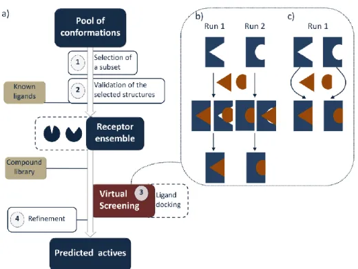
Virtual Screening is a computational strategy based on ligand docking, aimed to reduce the large virtual space of chemical compounds to a more reasonable number for further synthesis and pharmacological tests against biological targets of interest, which could lead to potential drug candidates. The Ensemble-based Virtual Screening is based on using multiple protein conformations in a docking study. Receptor structures from X-ray, NMR studies or homology models can represent the starting geometries to be used as they are, or as input for computational methods to generate multiple conformations. An extensive overview of such in
silico tools has been depicted in the previous section. Figure 4a below describes the
main steps of this protocol.
Figure 4. a) Schematic representation of the Ensemble-based Virtual Screening. b) and c) Combinations of multiple conformations in an Ensemble-based Virtual Screening.
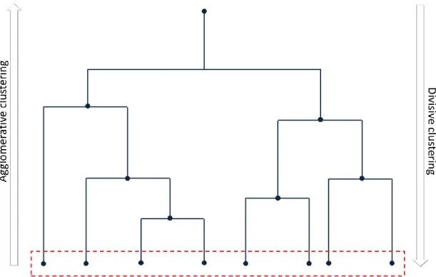
18 Step 1. The pool of conformations is analyzed, in order to select the most biologically relevant structures. It is possible to extract conformations from MD or MD-based simulations at regular intervals, but this approach may introduce redundancy and low structural diversity. In alternative, clustering methods are widely used to select representative conformations for Virtual Screening.65, 91 Several criteria can be used to cluster multiple structures, such as structural similarity in terms of RMSD values. To focus on the most significant geometries, this parameter may be calculated on regions of interest like the binding site, residues involved in binding mode or flexible protein domains linked with the active site. The selection of pairwise metric, clustering metrics and atoms used for the comparison can strongly affect the cluster analysis performance. Although cluster algorithms give generally satisfying results, they can exhibit limitations, such as the tendency to generate small, singleton or homogeneously sized clusters or the low stability to noise and changes in clustering parameters.92 Alternatively, reduced dimensionality of data can be exploited to manage reasonable numbers of conformations.93 For example, after long MD simulations, the most relevant degrees of freedom can be obtained by the Principle Component Analysis.94 Network analysis is another emerging tool to analyze protein dynamics allowing to extract information regarding not only the structural diversity but also connectivity of the collected conformations.95
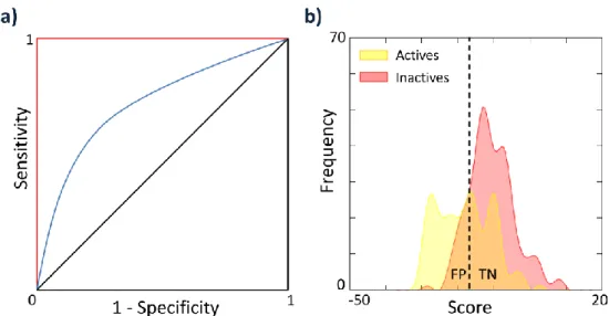
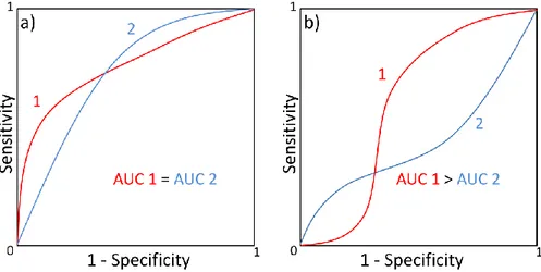
Step 2. Subsequently, the selected conformations are validated through ligand docking. In particular, a set of known active and inactive chemicals are docked in all the single structures of the ensemble. The goal of this retrospective study is to assess the predictive power of the conformations belonging to the final ensemble in perspective of the Virtual Screening. Several metrics can be used, including the Receiver Operating Characteristic and corresponding Area Under the Curve (ROC and AUC, respectively).96 These parameters describe the probability that actives will be ranked earlier than inactives in a rank-ordered list, as obtained after a docking run. This analysis can be useful to know if docking results bring added value compared to the random picking of compounds. In fact, this scenario should be translated in a real Virtual Screening, where a small proportion of the best ranked compounds is selected for biological tests. A good early recognition in a retrospective docking results in a high probability to find active compounds among the small proportion of ligands selected for experiments.
19 Sometimes, the validation study is used directly to select conformations, skipping step 1. In other words, the collected conformations are subject to a retrospective Virtual Screening and the best performing structures are selected based on their early recognition capability. However, the applicability of this procedure is restricted to a few ligands and a low number of protein conformations. In fact, a retrospective docking study of thousand ligands on large number of conformations collected by long Molecular Dynamics simulations as such, maybe computationally demanding. An example of this application is the ALiBERO protocol, recently developed by Rueda et al.97 It is based on EN-NMA Monte Carlo simulations to collect multiple conformations, and selects the best pockets maximizing the recognition of ligand actives from decoys.
Step 3. The validated conformations are then used for docking a ligand database. Several docking software and scoring functions are available and are used to rank large numbers of ligands and identify hit compounds. Multiple conformations can be combined in an Ensemble-based screening in two different ways: i) independent docking runs and selection of the best ranked pose for each ligand in one of the collected conformations, or ii) a single docking run with all the protein structures.87 Figures 4b and 4c schematize these procedures.
Compounds used for docking are selected from databases of commercially-available compounds98 consisting of large number of molecules (≈ 106, 107), filtered out according to drug-likeness or lead-likeness criteria, which are based on the Lipinski‘s rule of five.99
These filters ensure that molecules will be chemically stable and reduce risk of toxicity. Substructure filters to remove Pan Assay Interference Compounds (PAINS), or promiscuous compounds are also used.100-101 Step 4. A lead optimization phase can follow the hit identification, with the goal to improve binding affinity with more sophisticated and accurate methods. Molecular mechanics/generalized Born surface area (MM/GBSA)102 and the molecular mechanics/Poisson-Boltzmann surface area (MM/PBSA)103 are efficient techniques in calculating free energy of binding by means of molecular mechanics force fields and continuum solvent models. They can be used in conjunction with scoring functions or in a postprocessing step to enhance ranking and binding energy prediction of ligands.104 In the lead optimization step, the most popular computational technique is the Free Energy Perturbation (FEP), a very useful tool for guiding molecular design. This method consists of alchemic transformations
20 between two states, in conjunction with MD or Monte Carlo simulations in implicit or explicit solvent. Alchemic free energy methods are efficient and accurate but computational demanding. Moreover, an optimal accuracy is obtained only within a congeneric series of compounds.
1.5 AIM OF THE WORK
The dynamic character of proteins strongly influences biomolecular recognition mechanisms. With the development of the main models of ligand recognition (lock-and-key, induced fit, conformational selection theories), the role of protein plasticity has become increasingly relevant. In particular, major structural changes concerning large deviations of protein backbones, and slight movements such as side chain rotations are now carefully considered in drug discovery and development. In the light of what described so far, it is of great interest to identify multiple protein conformations as preliminary step in a screening campaign. Through the projects described in details in the Chapters 3 and 4, protein flexibility has been widely investigated, in terms of both local and global motions, in two diverse biological systems. On one side, Replica Exchange Molecular Dynamics has been exploited as enhanced sampling method to collect multiple conformations of Lactate Dehydrogenase A (LDHA), an emerging anticancer target. The aim of this project was the development of an Ensemble-based Virtual Screening protocol, in order to find novel potent inhibitors.105 On the other side, a preliminary study concerning the local flexibility of Opioid Receptors has been carried out through ALiBERO approach, an iterative method based on Elastic Network-Normal Mode Analysis and Monte Carlo sampling. Comparison of the Virtual Screening performances by using single or multiple conformations confirmed that the inclusion of protein flexibility in screening protocols has a positive effect on the probability to early recognize novel or known active compounds.
21
2. METHODS
2.1 MOLECULAR MODELING
Molecular modeling is the ensemble of all theoretical and computational methods required to describe and evaluate the properties of biological systems. These methods represent an important tool to investigate and better understand experimental data, gain knowledge on molecular structures and biological mechanisms, systematically explore structural/dynamical/thermodynamic patterns, etc. Experimental structures from X-ray or nuclear magnetic resonance provide the basic elements for molecular modeling. In fact, they are often used as starting point to study biological mechanisms, protein flexibility, energetic contributions to ligand-protein interactions, etc. In general, all methods of which molecular modeling takes advantages allow atomistic level description of the molecular systems, at different degrees of detail. Mainly, molecular modeling uses two different approaches: quantum mechanics and molecular mechanics. The former approach aims at solving the Schrödinger equation for each atom of the system, in order to explore the electronic structure of molecules. In other words, nuclei and electrons are explicitly treated. On the one hand, it results in a very accurate and robust method and produces a high level of detail of the phenomenon under investigation. However, it requires long calculation time with a considerable computational effort, especially for systems consisting of a large number of atoms, then limiting its applicability to specific cases, such as reaction mechanisms in which few atoms are involved. When biological systems consisting of hundreds to even thousands atoms are taken into account, the Molecular Mechanics (MM) turns out to be a more appropriate approach. It allows to evaluate the energy of a system as a function of the nuclear positions only, while electrons are implicitly considered through an adequate parameterization of the potential energy function.
2.2 MOLECULAR MECHANICS AND FORCE FIELD (FF)
Molecular Mechanics is regularly used when the biological system of interest contains a significant number of atoms, although some properties depending on electronic distribution are better treated with quantum mechanical approaches. The Born-Oppenheimer approximation is a fundamental principle that allows to
22 consider the energy as function of nuclear coordinates only.106 Nuclei that are heavier in terms of mass compared to electrons, are characterized by negligible velocity. It means that they are considered stationary with electrons moving around them. In the light of this phenomenon, the Born-Oppenheimer approximation states that the Schrödinger equation can be split into a part describing the electronic motions and the other regarding the motions of the nuclei, resulting in two independent wave functions. Molecular mechanics treats a molecule as a collection of masses interacting each other through harmonic forces. In other words, atoms can be simplified as hard spheres with radii obtained from experimental or theoretical data and net charges, while bonds can be represented as springs. In this way, many of the laws of classical mechanics can be applied for studying biological systems of any size in reasonable computational time. The different types of forces holding together all the atoms within the molecule are described by different terms of potential functions which, summed together, define the molecular potential energy, referred to as Force Field (FF). These terms are connected to changes in internal coordinates, that is bond lengths, angles and rotational or dihedral angles.
A relevant property of Force Fields is the transferability, that means the ability to use the same functional form and parameters to describe several systems, instead of defining specific functions for each single molecule. In this way, it is possible to use the Force Field to reproduce and predict structural properties of a wide range of molecules, although some specific systems require particular models. To this end, it is important to highlight that Force Fields are empirical, in other words a ―perfect‖ form does not exist. Most of the available Force Fields are based on the same functional form, suggesting that a generic model is possible. Actually, this similarity is only due to evaluation of comparable interactions in a system. Especially when novel chemical classes are explored, the appropriate Force Field needs to be defined or, in alternative, chosen carefully. The choice of the most appropriate function depends also on the compromise between accuracy and computational efficiency. Force Fields express parameters in terms of atom types to define atoms of the system of interest. In particular, atom types describe hybridization states and neighboring environment, for example to distinguish atoms of histidine amino acid based on its protonation state or sp3- from sp2-hybridized carbon atoms.
23 Force Fields can be simplistically defined as the sum of four different terms including all the intra- and inter- molecular interactions within a system, as reported below:
(1)
Vtot(r) is the potential energy of a system as function of the atom positions (r). The
first three contributes are relative to deviations of the internal coordinates from reference values and, then, refer to atoms directly bound (for this reason defined bonded terms). In details, the first and second terms (stretching and bending) are modeled as harmonic potentials and describe the energy when bond lengths and angles deviate from the reference values, whereas the third term is referred to changes in energy when rotations around bonds occur. The fourth contribute is referred to as non-bonded term and treats the interactions of non-bonded parts of the system. It is calculated for atoms separated by at least 3 bonds and usually concerns electrostatic interactions modeled using Coulomb potential and van der Waals interactions by a Lennard-Jones potential. Additional terms are sometimes included in sophisticated Force Fields.
In particular, the bond stretching and angle bending are calculated through Hooke‘s law as follows:
(2)
(3)
where k is the force constant and r0 is the reference bond length for the first
contribution, while k and θ0 in Eq. (3) are the force constant and the reference
angle. In consideration of the strong forces interacting between atoms, energy necessary to deviate a bond from its equilibrium value is high, resulting in large force constants for this contribute. On the contrary, force constants for the angle bending are lower because less energy is required to distort angles from their equilibrium position. In general, bond lengths and angles are defined ―hard‖ degrees of freedom because high energy is required to deform them, compared to the remaining contributions. Structural modifications mainly regard torsional and non-bonded contributions.
24 The torsional potential expresses the rotational energy about a bond as reported below:
(4)
with ω that is the torsional angle, is the barrier of rotation (the barrier height), n is the multiplicity, that is the number of minima in the function when bond rotates through 360° and finally, γ is the phase factor that indicates where the angle passes through its minimum value. Improper dihedral angles are also considered to select the correct geometry of particular atoms and an out-of-plane bending term is included in the Force Field equation.
As regards non-bonded terms, they are usually treated as function of the inverse power of the distance. The electrostatic contribution is defined through the Coulomb law:
(5)
where NA and NB are the point charges in the molecules A and B, 1/4πε0 is the
Coulomb‘s constant and rij is the distance between the two charges. These
interactions involve pair atoms, resulting in what is known as pairs potentials that require long calculation time. Another limitation is related to the definition of partial charges to calculate the Coulomb energy that are not a directly observable property of an atom and not a property that can be measured directly by experiment. Then, it cannot be unambiguously defined and several methods are available to determine partial charges that reproduce desirable molecular properties. Finally, the van der Waals potential describes the dispersions and repulsions between atoms. One of the most used functions to describe van der Waals interactions is the Lennard-Jones 12-6 equation:
25 with ε and ζ corresponding to the collision diameter and the well depth, respectively. The term powered to 12 describes the repulsive forces between the electronic distributions of two atoms that are close each other. The second contribute is the attractive long-range term that derives from London dispersion forces between induced dipoles for atoms with electron dispersion. Similarly to the electrostatic term, pair potentials are used to study the van der Waals interactions, leading to the evaluation of a huge number of interacting elements.
2.3 GENERATING CONFORMATIONAL ENSEMBLE
2.3.1 MOLECULAR DYNAMICS
Molecular Dynamics (MD) evaluates the ―real‖ dynamics of a system through the integration of the Newton equation of motion for an ensemble of particles and results in a trajectory over a given time. MD is a deterministic method, that is predictions of subsequent states can be defined from the current state. At defined steps, forces acting on the atoms are calculated and new positions and velocities are defined. Through MD simulations, microscopic properties are investigated, although macroscopic features are of major interest. The relation between microscopic and macroscopic features is at the basis of the statistical mechanics, composed of basic principles necessary to understand the theory of Molecular Dynamics.
A microscopic state is identified through the positions and momenta of the N elements forming the system. These properties represent the coordinates in a 6N-dimension space (each element is associated with 3 position variables and 3 momentum variables), referred to as phase space. Therefore, the system is defined as a point in this multidimensional space evolving over time, resulting in a trajectory in the phase space. According to the principles of statistical mechanics, the instantaneous value of an observable A depends on the momenta (pN) and positions (rN) and can be reported as follows:
(7)
Since this value fluctuates over time, due to the interactions between the particles, a time average (Aave) of A(t) is defined as the time increases to infinity:
26 (8)
From this equation, it is clear that to define average values of the observable A, it is necessary to describe dynamically the system in an infinite time. Obviously this is not feasible, especially if it is considered that macroscopic systems include a high number of atoms or molecules. To this end, the conventional approach of statistical mechanics considers a collection of systems (replicas) with the same macroscopic properties, instead of trajectories of a single system in the phase space. Each of these replicas is a point in the phase space and all together, they constitute what is known as statistical ensemble. Replicas progress in the phase space by keeping constant the thermodynamic properties which define the statistical ensemble. According to these constant properties, statistical ensembles can be classified in: canonical (NVT), microcanonical (NVE), isothermal-isobaric (NPT) and grand canonical (μVT). The thermodynamic properties of interest refer to number of particles (N), volume (V), energy (E), temperature (T), pressure (P) and chemical potential (μ).
Replicas are distributed based on a probability density, that is the probability to find a configuration with momenta pN and position rN. It is computed in different ways depending on the statistical ensemble under investigation. For example, in canonical ensembles in which energy fluctuations are observed, the density distribution is defined by the Boltzmann distribution:
(9)
where E(pN,rN) is the energy, 1/kBT is Boltzmann‘s constant with T standing for
temperature and Q is the partition function. The latter, as reported in Eq. (10), is the sum of the Boltzmann factors from all microstates and is used in the previous formula as normalization factor.
27 It can be treated with a classic or quantum mechanical approach. In other words, it can be expressed as sum of all the Boltzmann factors (as shown in the previous formula) or as integral in the 6N dimensional space.
In the microcanonical ensemble, energy is constant and all microstates are equiprobable. All replicas explore each point in the phase space due to their constant energy and then, the time average coincides with an ensemble average. This equivalence, as reported in Eq. (11), is at the basis of the ergodic hypothesis which is a fundamental axiom of statistical mechanics.
(11)
where
(12)
with M corresponding to the number of time steps and angle brackets indicating an ensemble average. Molecular Dynamics takes advantage of this hypothesis through the integration of the ensemble average in order to obtain the thermodynamic averages.
The Hamiltonian (H) controls the evolution of a system over time. It can be calculated for a system of N particles as the sum of kinetic energy K which only depends on p, and potential energy V only dependent on r. This second part is computed through the Force Field which has been discussed in the previous section. On the other hand, the kinetic energy has a simple quadratic form as reported below:
(13)
with mi corresponding to the mass of particle i and pix, piy, and piz the x, y and z
components of the momentum p, respectively. In an MD simulation, the evolution of the system over the time, controlled by the Hamiltonian H, is defined through the integration of the equation of motion. The forces acting on the atoms combined with positions and velocities at a given time step (t) allow to define new positions
28 and velocities at time interval t + Δt. Subsequently, atoms moves, forces are computed at the new positions and so on.
The Molecular Dynamics protocol consists of three main steps: minimization, equilibration and production. The starting structure of the system of interest and then, the resulting minimized geometry are the underlying configurations about which fluctuations occur during the simulation. Therefore, it is important to define a stable energy structure, that is a minimum on the potential energy surface to start the dynamics. For complex molecules, multiple minima are possible, as well as a global minimum may be identified, but in this case a conformational search would be needed. In order to reach the convergence, macromolecules are subject to large numbers of minimization iterations. Two examples of widely used minimization algorithms are the Steepest Descent and Conjugate Gradient. In the subsequent equilibration step, initial velocities are assigned to the atoms. Typically, they are randomly generated through a Maxwell-Boltzmann distribution. Random velocities can lead to a nonzero net momentum, resulting in possible translations or rotations of the system. Thus, in order to limit this effect, velocities are zero mean. Subsequently, the system is initially simulated to reach the equilibrium of the initial conditions. If the simulation is run at constant temperature, the system should be brought to the temperature of interest. During this step, in the light of the relation between temperature and velocity, this latter is rescaled until the desired temperature is reached. Once the properties of interest (V, T, P, E) show stable behavior in the equilibration step, the production can finally begin.
In an ideal system, we should consider lattice which is infinite in all dimensions. However, for computability and complexity reasons, some boundary conditions are necessary in order to simulate a part of an infinite system. As consequence, some molecules of the system are close to the edge of the sample and may be affected by surface effects which can be avoided by using Periodic Boundary Conditions. The box which includes the system of interest is replicated in different directions resulting in a periodic lattice of identical subunits. In this way, molecules located in proximity of the edge interact with the atoms of the neighboring box. In order to avoid that particles see their own periodic images, the minimum image convention is applied. According to this condition, each atom is surrounded by a box which is identical in size and shape to the periodic box and includes the remaining other atoms in the simulation. However, the calculation of the pairwise interactions of a
29 particle with all of the other particles in the system may be too expensive in terms of computational cost. In order to limit this problem, the potential truncation is used, that is the introduction of a cutoff within which the non-bounded interactions are calculated. For consistency with the minimum image convention, the cutoff distance should be lower than half length of the box.
An important parameter in Molecular Dynamics is the time step, which defines how often the integration of the equations of motion is performed. Ideally, to reduce computational costs a large time step should be used. In practice, it is typically restricted to the femtosecond time scale. This value must be shorter than the period of the fastest motions in a system, like the oscillations of the hydrogen atoms. In order to reach a compromise between computational costs and accuracy, use of constraint methods, such as the SHAKE algorithm,107 allows to fix bond lengths and then, increase the time step. The Verlet algorithm108 is one of the most used finite difference methods, which approximate the positions and dynamics properties through Taylor series expansions. In particular, the Verlet algorithm determinates each position from the current position at time t and position at time t
– Δt as follows:
(14)
In the context described so far, where the total energy of a system is conserved, the MD simulations explore the microcanonical ensemble (NVE). To simulate also the other statistical ensembles, like the isothermal-isobaric (NPT) or the canonical (NVT) ones, the equation of motion should be modified. In these further ensembles, velocities can be rescaled at certain steps so as to reach the desired target temperature, as already introduced earlier. In the isothermal-isobaric ensemble, constant pressure involves volume fluctuations. In this case, a target pressure is maintained by rescaling the simulation volume, through the use of a barostat. The Berendsen thermostat/barostat is widely used to weakly couple the system to an external heat bath with coupling constant for temperature and pressure.109 The Langevin thermostat is another example that adds a friction term and a fluctuating force to Newton‘s second law which is then integrated numerically.110 Details of these algorithms can be found in the related reference papers.