Microwave radars for short-range applications: from the transistor characterization to the system development

M

EDITERRANEAN

U

NIVERSITY OF

R

EGGIO

C

ALABRIA

U

NIVERSITY OF

M

ESSINA

D

EPARTMENT OF

E

NGINEERING

D

OCTORAL

P

ROGRAM IN

“I

C

,

A

S

”

Curriculum:

SCIENZE E TECNOLOGIE, MATERIALI, ENERGIA E SISTEMI COMPLESSI PER IL CALCOLO DISTRIBUITO E LE RETI

M

ICROWAVE RADARS FOR SHORT

-

RANGE APPLICATIONS

:

FROM THE TRANSISTOR CHARACTERIZATION TO THE

SYSTEM DEVELOPMENT

Doctoral Dissertation of:

Emanuele Cardillo

Supervisor:

Prof. Alina Caddemi

The Chair of the Doctoral Program:

Prof. Felice Arena

I

Contents

Contents ... I Acknowledgements ... III

Introduction ... 1

1 Micro-radars for short-range applications ... 2

Radar basics and technologies ... 2

1.1.1 Pulsed and continuous wave radars ... 4

1.1.2 Frequency-modulated continuous-wave radar ... 6

Radar subsystems ... 9

1.2.1 Radar transmitter ... 10

1.2.2 Radar antennas ... 10

1.2.3 Radar receiver ... 11

Threshold for targets detection ... 13

Micro-radar for short-range applications ... 15

1.4.1 Design and simulation ... 16

1.4.2 Realization and measurements ... 19

1.4.3 Transmitter linearization ... 23

A novel approach for crosstalk minimization... 25

A special application: a microwave white cane for visually impaired people ... 27

References ... 34

II

Noise ... 38

Noise in microwave transistors ... 40

2.2.1 Microwave transistors ... 46

2.2.2 Microwave GaAs-based transistors under light exposure ... 48

2.2.3 Microwave GaN-based transistors under light exposure ... 66

Low-noise amplifiers ... 76

2.3.1 Design, realization and performance of the low-noise amplifier prototype 82 2.3.2 Analysis of low-noise amplifiers under light exposure ... 92

2.3.3 LNA prototype under light exposure ... 102

References ... 111

3 Microwave filters ... 116

Filters in radar receiver ... 116

Extra wideband filters for microwave applications ... 119

References ... 130

Conclusions ... 132

Abbreviations and Symbols ... 134

III

Acknowledgements

I would like to express my sincere gratitude to my advisor Prof. Alina Caddemi, for giving me the opportunity of working in the Microwave Electronic laboratory, for her motivation, knowledge and experience not only in the microwave field but in the side activities too.

A special thank is due to Dr. Giuseppe Salvo and Prof. Giovanni Crupi for their help and stimulating discussions, as well as to Prof. Salvatore Patanè for his fundamental contribution in the experimental part of this work concerning the optoelectronic setup.

Last but not least, I would like to thank my family for supporting me throughout my Ph.D. course and for following me in my adventures.

1

Introduction

The microwave engineering history was likely born with the electromagnetic theory formulated in 1873 by James Clerk Maxwell, whereas one of its first major applications, the radar, was deeply studied and developed during the World War II. During the last decades, the microwave engineering has made a great leap forward due to the increasing number of applications, e.g. satellite communications, wireless and communication systems, radars, environmental remote sensing, cooking of food and medical systems.

The work of this Ph.D. course has been developed within the framework of the research activities of the Microwave Electronics (ELEMIC) laboratory of the University of Messina. As a consequence, the topics treated in this thesis have in common the analysis, design, realization and test of low-noise, high sensitivity microwave components and circuits. The central idea has been that of carrying out a multilayer analysis of a microwave short-range radar. First of all, the radar has been analyzed from a system-level point of view. As well as the main radar applications, technologies and circuital topologies, the research activity has been focused on the improvement of the digital signal processing techniques and on the prototyping and testing methods. In addition, a special application of the radar prototype has been developed with the purpose of enhancing the life quality of visually impaired people.

Thereafter, the problem of noise in radar receivers has been considered and, an in-depth investigation on the noise in microwave transistors has been carried out. GaAs- and GaN- based devices have been characterized not only without optical illumination conditions but also under the special condition of the light exposure. A microwave low-noise amplifier has been designed, realized and tested. Its behavior has been analyzed under light exposure too, for different wavelengths and radiation power levels. Finally, the problem of filtering in microwave receivers has been dealt with and a microwave filter with an extra wide bandwidth has been designed, realized and tested.

The present thesis is organized into three Chapters. In Chapter 1, the micro radar for short-range applications is described along with design and test details. Chapter 2 provides a deep investigation of noise in radar receivers and in Chapter 3 microwave planar filters are analyzed. Finally, the conclusions are drawn and some directions for feasible research developments are proposed.

2

1 Micro-radars for short-range applications

This Chapter briefly reviews the main radar technologies and architectures. Thereafter, the design, simulation, realization and test of the proposed micro-radar are reported. Moreover, a novel approach for the minimization of crosstalk between the radar transmitter and receiver and a special application in the social context are presented.

Radar basics and technologies

During the last decades, radar systems have made a great leap forward, tremendously evolving their functions. Although the RADAR acronym “Radio Detection And Ranging” suggests applications in the field of the target detection and distance computing, modern radars are technologically advanced devices able of tracking, identifying and imaging targets in a limitless number of applications from civilian to military, from short to long range and with dimensions of targets from millimeters to tens of meters. A radar is essentially a system that transmits electromagnetic waves toward an area of interest and eventually receives the signals (echoes) reflected from objects (targets) for acquiring information about them. A typical radar schematic is reported in Fig. 1.1. It can be simpler or more complicated but, basically, it must include a transmitter, one or multiple antennas, a receiver and a signal processing section. The transmitter is responsible for generating the electromagnetic signal, whereas the antenna is the transducer that permits the propagation in the atmosphere and vice versa. In some cases, a circulator can be used for providing the connection between the transmitter and the antenna during the transmission time and between the antenna and the receiver during the receiving time. Moreover, it shields the very sensitive components of the receiver from the transmitted signal, thus improving the isolation. If a unique antenna is used for detecting the signal, the radar configuration is monostatic, otherwise it is bistatic. The target, possibly together with other objects, reradiates the induced electromagnetic field in the space. The unwanted unintentional and intentional reflected signals are called clutter and jamming, respectively. The captured signal is then amplified by a low-noise amplifier, converted into an intermediate frequency (IF) and, after an analog-to-digital conversion, finally processed [1].

3

Fig. 1.1: Typical radar schematic [1].

A fundamental radar figure of merit is the maximum detectable range. It depends on several factors, e.g. the radar mode of operation, its characteristic parameters and the properties of the target. The last ones are usually accounted by the radar cross section (RCS) parameter, i.e. a measure of power scattered in a given spatial direction when the target is illuminated by the transmitted signal.

The relationship modelling the amount of received power (𝑃𝑟) as a function of system specifications and target features is reported in eq. (1.1):

𝑃𝑟 = 𝑃𝑡𝐺𝑡𝐺𝑟𝜆2𝜎 (4𝜋)3_𝑅4_𝐿 𝑠 (1.1) where:

𝑃_𝑡 is the peak transmitted power (W); 𝐺_𝑡 is the transmitting antenna gain; 𝐺𝑟 is the receiving antenna gain;

𝜆 is the wavelength of the transmitter signal (m); 𝜎 is the radar cross section of the target (m2_); 𝑅 is the distance from the radar to the target (m);

𝐿_𝑠 is the sum of transmitting, atmospheric, receiving and signal processing losses; The receiver thermal noise (𝑃_𝑛) is given by eq. (1.2):

4

𝑃𝑛 = 𝑘𝑇0𝐹𝐵 (1.2)

where:

𝑘 is the Boltzmann’s constant in watt-per-seconds/Kelvin; 𝑇₀ is the standard temperature in Kelvin;

𝐹 is the noise factor;

𝐵 is the receiver bandwidth in Hertz;

The minimum detectable signal (MDS) for obtaining the required signal-to-noise ratio (SNR) is given by eq. (1.3):

𝑀𝐷𝑆 = 𝑃𝑛∙ 𝑆𝑁𝑅 = 𝑘𝑇0𝐹𝐵 ∙ 𝑆𝑁𝑅 (1.3) where 𝑆𝑁𝑅 is the signal-to-noise ratio.

Solving Eq. 1.1 for determining 𝑃𝑟 and replacing it with the MDS, it is possible to obtain the maximum detectable range, 𝑅_𝑚𝑎𝑥, as shown in eq. (1.4):

𝑅_𝑚𝑎𝑥 = 𝑃𝑡 𝐺𝑡 𝐺𝑟 𝜆 2 _𝜎 (4𝜋)3 _𝐿

𝑠 𝑆𝑁𝑅 𝑘 𝑇0 𝐹 𝐵

(1.4)

1.1.1

Pulsed and continuous wave radars

Radars can be classified into two categories depending on the transmitted waveform: continuous wave (CW) and pulsed radar.

The formers transmit and receive continuously the signal, usually employing a bistatic configuration.

Since it transmits without interruptions, the determination of the target range is not possible. Consequently, the CW radar is usually employed for detecting the radial velocity of a target. Actually, the range detection is possible with a CW radar by modulating the transmitted signal, as it will be explained in the next section.

If the target is moving, the frequency of the received wave will be different from the frequency of the transmitted one. This effect is commonly known as Doppler Effect and the related Doppler frequency shift 𝑓𝑑 is given by eq. (1.5):

5 𝑓_𝑑 = 2𝑣𝑟

𝜆

(1.5)

where 𝑣𝑟 is the radial velocity of the target.

The radar takes advantage from the Doppler Effect, calculating the frequency shift and consequently the radial velocity by adopting a homodyne receiver. The inputs of the mixer are the signal of the local oscillator and the received echo. Therefore, the frequency of the intermediate frequency signal, after a low-pass filtering, is exactly equal to the Doppler shift. By properly selecting the main radar parameters it is possible to make feasible the analog-to-digital conversion, thus easily calculating the IF frequency.

The signal transmitted by a pulsed radar is an EM wave with a very short duration, called pulse width (τ) that can range from few nanoseconds to few milliseconds, depending on the application. Usually, during the transmission, the receiver is isolated from the transmitter in order to protect its very sensitive components. Since no echoes can be received during this time, this will affect the minimum detectable range. The pulse width plus the receiving time is called Pulse Repetition Interval (PRI), whereas the number of completed cycles per second is called Pulse Repetition Frequency (PRF). They are related according to eq. (1.6):

𝑃𝑅𝐹 = 1 𝑃𝑅𝐼

(1.6)

These quantities are illustrated in Fig. 1.2.

Fig. 1.2: Typical pulsed transmitted waveform [1].

By measuring the time delay (∆𝑇) between the transmitted and the received signal, the target range can be determined with the well-known relationship expressed in eq. (1.7):

6 𝑅 =∆𝑇𝑐

2

(1.7)

where c is the speed of light in vacuum.

Since the radar timing affects the minimum detectable range, it can affect the maximum detectable range in the same way. Indeed, if the pulse round-trip time is greater than the PRI, the echo will not return to the radar before of the next pulse transmission. Therefore, the received signal might be a reflection of the last pulse from a close target, or a reflection of the previous pulse from a distant target, thus resulting in a range ambiguity.

Finally, the spatial resolution 𝛿𝑅 of a pulsed radar can be expressed as reported in eq. (1.8):

𝛿𝑅 = 𝜏𝑐

2

(1.8)

1.1.2

Frequency-modulated continuous-wave radar

For a certain number of applications, the traditional continuous wave and pulsed technologies are not suitable for resolving the target range and/or speed. For instance, the pulse round-trip time for detecting a target placed at the distance of 5 m with a pulsed radar corresponds approximately to 33 ns. Considering Eq. 1.8, the same pulse width must be employed for detecting a farther target with a spatial resolution of 5 meters. This shorter pulse duration would require an expensive and complex transceiver. In addition, shorter pulses have less energy and make the target detection more difficult.

The frequency-modulated continuous-wave radar (FMCW) is a particular radar technology that, even though based on a continuous wave technique, puts a timing mark on the EM wave, thus allowing the target range determination. In addition, the spatial resolution is managed in terms of the frequency modulation bandwidth avoiding the requirement of very short pulses. The FMCW modulation has several advantages:

 The minimum detectable range is comparable to the transmitted wavelength.  The resolution of the range measurement is very high.

 It allows both target range and radial velocity measurement.  The required signal processing architectures are relatively simple.  High power pulses are not needed, thus improving safety operations.

7 The range delay has to be measured indirectly, computing the frequency or phase difference between the transmitted and received signal. Different modulation patterns can be employed depending from the application. Hereafter, the most used saw-tooth and triangular modulation will be analyzed in details.

A typical saw-tooth frequency shape is reported in Fig. 1.3. The time delay of the received signal results in a difference between the transmitted frequency and received one. The frequency difference is called beat frequency and it is a measure of the distance of the reflecting object. If the target is moving, the Doppler shift changes the frequency of the received signal either up or down, for motion directed towards or away from the radar, respectively.

Fig. 1.3: Transmitted (solid line), received (dashed line) and beat (dotted line) frequency waveform vs time [2].

From Fig. 1.3, considering ∆𝐹 as the peak-to-peak bandwidth and 𝑇_𝑚 as the modulation period, it is easy to geometrically establish the relationship expressed in eq. (1.9):

𝑓𝑏 ∆𝑇=

∆𝐹 𝑇_𝑚

(1.9)

where 𝑓𝑏 is the beat frequency in Hertz.

By using Eq. 1.7 together with Eq. 1.9, it is possible to relate the beat frequency with the range, as shown in eq. (1.10) [2]:

8 𝑓_𝑏 =∆𝐹 𝑇_𝑚 2𝑅 𝑐 (1.10)

Clearly, the receiver cannot distinguish between the beat and the Doppler frequency, thus affecting the distance calculation. Anyway, this modulation is considered to be Doppler tolerant, having a negligible influence of the Doppler frequency for several application, e.g. a maritime navigation radar [2], [3]. By considering the characteristics of both the radar and the application proposed in this thesis, the Doppler mismatch will induce very small errors, while preserving the mainlobe and sidelobe structures. Indeed the analyzed targets are almost stationary or they can move very slowly. As stated before, the target resolution can be expressed in terms of the linear frequency modulation range, as reported in eq. (1.11):

𝛿𝑅 = 𝑐 2 ∆𝐹

(1.11)

Coming back to the example at the beginning of this section, for obtaining a resolution of 50 cm, ∆𝐹 = 300 𝑀𝐻𝑧 is required. With a modern radar transceiver, this or even wider linear modulation bandwidths can be easily obtained.

If the separation between the difference frequency ∆𝐹 and the Doppler frequency 𝑓_𝑑 is required, the triangular modulation pattern can be used. The reflected signal is shifted due to the round-trip time. Without a Doppler shift, the frequency difference during the rising edge is the same as the difference during the falling edge.

If a Doppler shift occurs, two different frequencies appear for the rising edge and for the falling edge. Considering the upsweep 𝑓_𝑏𝑈𝑃 and downsweep 𝑓_{𝑏𝐷𝑊𝑁} beat frequencies given by eq. (1.12) and eq. (1.13), the range and velocity can be expressed as reported in eq. (1.14) and eq. (1.15), respectively [2]: 𝑓𝑏𝑈𝑃 = −∆𝐹2𝑅 𝑇_𝑚𝑐 + 2𝑣_𝑟 𝜆 (1.12) 𝑓_{𝑏𝐷𝑊𝑁} = ∆𝐹2𝑅 𝑇_𝑚𝑐 + 2𝑣_𝑟 𝜆 (1.13) 𝑅 = 𝑇𝑚𝑐 2 ∆𝐹(𝑓𝑏𝐷𝑊𝑁− 𝑓𝑏𝑈𝑃) (1.14)

9 𝑣_𝑟 = −𝜆

4 (𝑓𝑏𝐷𝑊𝑁+ 𝑓𝑏𝑈𝑃)

(1.15)

With a triangular-shaped waveform, after a digital signal processing, both an accurate range and velocity determination can be performed. On the other hand, if multiple targets exist, the measured frequencies cannot be uniquely associated with each target, thus leading to ghost targets. With an increased complexity of the transmitter and of the signal processing section, this issue can be overcome by measuring cycles with different slopes.

Radar subsystems

For an in-depth analysis of the radar subsystems, a more detailed block diagram of a radar is reported in Fig. 1.4. The figure is referred to a pulsed radar, but the following considerations about the main blocks can be considered general.

10

1.2.1

Radar transmitter

The radar transmitter is the subsystem that generates the electromagnetic waves required for illuminating the target. The transmitter’s configuration varies depending on the specific application in terms of transmitted signal pattern, power level, timing and technology. Radars can be classified in coherent and non-coherent. The former needs to employ a very stable oscillator for having a well-known phase of the transmitted signal. On the other hand, the latter configuration is less complicated from both hardware and signal processing requirement and consequently much cheaper to implement. Another important choice involves the RF source selection, with two main options based on vacuum tubes or on solid-state devices.

The general trend is to replace the vacuum tube-based RF sources with solid-state devices because of the potentially higher performance, reliability, maintenance costs and smaller dimensions of the last ones. Obviously, there are many applications where solid-state devices cannot compete with vacuum tube devices in terms of output power, efficiency and cost, e.g. when hundreds of kilowatts of average power are required. Finally, modern radars require the modulation of the RF signal, e.g. for FMCW or pulse compression techniques, together with a proper selection of a suitable power supply [4].

1.2.2

Radar antennas

The antenna is the transducer that launches the propagation in the surrounding environment and vice versa. It has a great impact on the radar performance, i.e. only target within the antenna field of view can be detected. The antenna effects on the radar performance are quite clear by observing eq. (1.4) in which the gain terms have a great influence. In Fig. 1.5, the radiation or directivity pattern of an antenna together with some related parameters are shown. One of the most important figure of merit is the 3 dB beamwidth, i.e. the angle between the two -3 dB points on the two sides of the main beam. Moreover, two fundamental parameters are the directivity and the gain. The former is a dimensionless parameter defined as the ratio of the radiation intensity at the main beam peak divided by the radiation intensity of a lossless isotropic antenna with the same radiated power. The latter is defined as the ratio of the radiation intensity at the main beam peak divided by the radiation intensity of a lossless isotropic antenna with the same input power, i.e. the maximum directivity multiplied by the antenna efficiency.

11

Fig. 1.5: Radiation pattern of an antenna [1].

The last parameter visible in Fig. 15 is the sidelobe level. The average sidelobe level is a very important parameter since strong sidelobes can increase the number of false alarms, for example due to clutter or jamming. The peak sidelobes are usually expressed in dBi (dB relative to an isotropic antenna).

1.2.3

Radar receiver

The echo, after the antenna detection, passes through the receiver section in order to achieve the desired information about the target. One of the receiver features is the capability of protecting its internal sensitive components from the relatively high power of the transmitter. Depending on the technologies, this task can be accomplished by a duplexer, e.g. a circulator eventually with a series protecting switch to disconnect the receiver during the transmission time. Afterwards, an amplification stage is required for increasing the received signal strength together with a low level of noise, which is accomplished by using a low-noise amplifier (LNA).

12 In addition, a RF preselection is often required for minimizing the exposure to spurious signals, by filtering or eliminating the interferences.

Usually, radars need to convert the received signal into a lower intermediate frequency for detecting or processing the information. The down-conversion process can be accomplished directly with a single stage or with multiple steps, e.g. double down-conversion process. Since for a single down-conversion stage the local oscillator (LO) frequency must be quite close to the high frequency received signal, spurious frequency can appear into the IF signal. Typically, these are due to small differences between the transmitted and the LO frequency or to the appearance of the image frequencies. With the first downconversion stage, the unwanted converted components are further separated from the RF, making it easier to filter them out. Finally, the analog-to-digital conversion is usually performed to perform a digital signal processing.

In designing a radar system, particular attention should be paid to the receiver dynamic range, namely the minimum and maximum signals that the receiver can correctly process. The lower limit is fixed by the noise floor, whereas the upper one is limited by the third-order intermodulation level of the amplifiers and mixers. Since a radar designer has to carefully select each receiver stage, different guides are available in scientific literature [5], [6]. For targeting a suitable dynamic range, two main tools are typically used: the sensitivity time control and the gain control. The former consists of decreasing the sensitivity of the radar for short-range echoes, the latter manually or automatically sets the gain of the receiver for enabling the detection of smaller targets. The last section in a radar receiver, preceding the signal processing stage, is the analog-to-digital data conversion block.

Modern radars employ different receiver configurations: crystal video, superregenerative, homodyne and superheterodyne receiver are the most famous [1]. In the radar system proposed in this thesis, a homodyne receiver has been used whose general schematic is reported in Fig. 1.6. The mixer local oscillator input is represented by a small portion of the transmitted signal. The circulator purpose is to either couple the transmitted signal with the antenna while isolating the receiver, and to couple the received signal with the receiver while isolating the transmitter. The mixer output, after being filtered and amplified, usually already contains the required information about the target.

Another local oscillator is not necessary, thus making this type of receiver simpler to realize and able of providing a coherent signal processing. It is often used for CW and FMCW radars.

13

Fig. 1.6: Homodyne receiver schematic [1].

Threshold for targets detection

The first task of a radar is the target detection that consists in determining if an echo is composed only by an interference or by an interference plus a target. The main criterion for radar detection algorithms usually is the Neyman-Pearson criterion [7]. It is based on two hypotheses:

 The analyzed signal is only an interference, null hypothesis (𝐻0).  The analyzed signal is an interference plus a target echo (𝐻₁).

Since the combined target plus interference signal is a random process, two probability density functions (PDFs) are required, as reported in eq. (1.16) and eq. (1.17):

𝑝𝑦(𝑦|𝐻0) = 𝑃𝐷𝐹𝑜𝑓 𝑦 (𝑡𝑎𝑟𝑔𝑒𝑡 𝑛𝑜𝑡 𝑝𝑟𝑒𝑠𝑒𝑛𝑡) (1.16)

𝑝𝑦(𝑦|𝐻1) = 𝑃𝐷𝐹𝑜𝑓 𝑦 (𝑡𝑎𝑟𝑔𝑒𝑡 𝑝𝑟𝑒𝑠𝑒𝑛𝑡) (1.17) The Neyman-Pearson criterion, after fixing the probability of false alarm PFA, is aimed at maximizing the probability of detection PD, for a given SNR. After reception of the echo, a threshold is computed and the echo level is compared with it. If the signal is beyond the threshold, it is assumed to be the target plus interference, otherwise it is assumed to be the interference only. The verb “assumed” is meaningful because it implies that the decision can

14 be wrong, leading to a false alarm. Since usually the higher the value of PD, the higher the value of PFA, a radar designer have to choose the maximum value of PFA that can be tolerated. The decision rule has been synthetized in the likelihood ratio test (LRT), as shown in eq. (1.18) [8]:

Λ(y) 𝐻₁ > < 𝐻₀ 𝑇_Λ (1.18)

where 𝑇Λ is the unknown threshold value, Λ is the likelihood ratio. and:

Λ(y) = 𝑝𝑦(𝑦|𝐻1) 𝑝𝑦(𝑦|𝐻0)

(1.19)

The likelihood ratio is a random variable with its PDF. Usually, a model for the PDF of the detections statistic (z) under 𝐻₀ is determined with the aim of finding the threshold value T so that the probability of y exceeding T is the desired PFA, as expressed in eq. (1.18) [1]:

𝑃_𝐹𝐴 = ∫ 𝑝_𝑧(𝑧|𝐻0)𝑑𝑧 +∞

𝑇

(1.18)

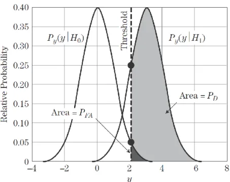
These concepts are depicted in Fig. 1.7, where the notional Gaussian PDF of the voltage y under 𝐻₀ and 𝐻₁ together with the PFA and the PD are reported.

For improving the system performance in terms of PD, a radar designer can operate on the antenna design, on the transmitted waveform and power level and on the signal processing technique. The last possibility has been implemented in the work of this thesis and it will be shown in section 1.6.

15

Fig. 1.7: Notional Gaussian PDF of the voltage y under H0 (left) and H1 (right), together with the PFA (black) and the PD (gray

plus black) [1].

Micro-radar for short-range applications

In this thesis, a micro-radar for short-range applications has been designed, realized and tested. The required specifications are:

 Range resolution: 15 cm;

 Minimum detectable range: as low as possible;  Maximum detectable range: 5 m;

 Lowest overall dimension;  Low consumption;

 Low price.

For fulfilling these requirements, a frequency-modulated technique has been adopted. The key trade-offs mainly consist of a proper selection of the transmitted frequency, modulation bandwidth, modulation period and beat frequency. The transmitted frequency has been selected in the 24-26 GHz bandwidth, which is typically used in the anti-collision automotive radars, allowing the reduction of the system dimension. The smaller the modulation bandwidth, the

16 lower the amplitude and the phase noise, whereas a higher modulation bandwidth allows obtaining a finer range resolution, a lower radiated power spectral density and a higher beat frequency.

In addition, by decreasing the modulation period, the beat frequency and the unambiguous velocity and range increase.

Finally, the effects of decreasing the beat frequency are: lower ADC sample frequency; range bin (the bin is the frequency point associated with each result vector element of a FFT) filter with narrower bandwidth; higher phase noise.

A linear saw-tooth signal with a modulation bandwidth of 1.1 GHz, from 24 to 25.1 GHz, has been selected, thus obtaining a spatial resolution of 15 cm. The chirped waveform has been shaped by using a modulating saw-tooth signal with a period of 2 ms. In addition, the transmitted signal has been pulsed, thus reducing the power consumption.

With the aim of achieving both a reasonable dwell time and a limited ON state period of the transmitter, the pulse duration has been chosen equal to 10 ms. Similarly, the pulse repetition time (PRT) has been selected equal to 100 ms, thus obtaining a duty-cycle of 10% that is a good compromise for saving energy and for guaranteeing a comfortable data refresh time.

The transmitted power has been set equal to 11 dBm that allows of obtaining the required maximum range of 5 m. These performances have been obtained by realizing a cost-effective system based on commercially available components and a microwave section based on microstrip technology that allows ease of integration with the antenna section as well as the prototype realization by using in-house facilities.

1.4.1

Design and simulation

For properly analyzing the radar behavior, an equivalent system has been simulated employing the Visual System Simulator™ (VSS) software of the NI AWR Design Environment™ platform. This analysis has been performed at the beginning of this study and the employed parameters are slightly different from the previous ones (frequency bandwidth from 24.5 to 25.5 GHz, PRT of 5 ms and pulse duration of 1 ms) [9]. Anyway, it has been very useful for understanding the main radar characteristics. The schematic of the whole system is reported in Fig. 1.8.

17 Every target is modelled by means of two blocks. The former reproduces the delay related to the roundtrip path of the wave reflected from the target, the latter adds the white Gaussian noise of the channel and variable losses for different target distances. Typical delays for distances among 1 m and 5 m vary from 6.7 ns to 33.3 ns. The presence of leakage from the transmitter section to the receiver one is also taken into account.

Fig. 1.8: Behavioral radar equivalent system [9].

Power and frequency of the transmitted signal are shown in Fig. 1.9.

Fig. 1.9: Power (blue solid line) and frequency (red dashed line) of the transmitted signal [9]. AMP_B BPFB FP1=24000 MHz FP2=26000 MHz LPFB FP=0.1 MHz 1 2 3 C2RI TP ID=I TP ID=Q TP ID=Tx 1 2 3 DCOUPLER_3 TP ID=chirp TP ID=Rx 1 PPULSE Sawtooth 1 SAW 1 2 3 4 SPDT_21 SRC_C 1 2 3 VCO_B TP ID=IF DELAY AMP_B GAIN=26 dB DELAY DELAY AWGN AWGN AWGN 1 2 3 DCOUPLER_3 IN OUT LO MIXER_B2 NF=12 dB 1 2 3 4 5 COMBINER ID=S8 I Q Att.: 75 dB Dist.: 3 m Dist.: 5 m Att.: 90 dB Att.: 55 dB Dist.: 1 m

Target

Transmitter

Receiver

18 In the receiver sections, the reflected signals are filtered, amplified and mixed with a replica of the transmitted ones, thus extracting the in-phase and quadrature components. The overall receiver single-sideband noise figure and gain are respectively 12 and 26 dB. The waveform and the spectrum of the IF signal are both reported in Fig. 1.10.

(a)

(b)

Fig. 1.10: (a) IF signal waveform and (b) spectrum [9].

The presented approach has been found to be highly flexible for various radar scenarios, by avoiding the typical restrictions due to the crosstalk noise.

19

1.4.2

Realization and measurements

After the preliminary simulation, the main parameters have been adjusted as described above. The radar prototype employs the BGT24MTR11 integrated circuit as leading block, a SiGe MMIC Transceiver by Infineon Technologies AG [10]. By means of its 24.0 GHz fundamental Voltage Controlled Oscillator (VCO), it can operate from 24.0 to 26.0 GHz, delivering a main RF output power of 11 dBm. The output signal is provided by a differential output. The chip is equipped with an SPI interface, thus allowing to be controlled by a Microcontroller Unit (MCU). Switchable frequency prescalers are included with output frequencies of 1.5 GHz and 23 kHz. A LNA provides low noise figure and a RC polyphase filter (PPF) is used for LO quadrature phase generation of the homodyne quadrature downconversion mixer. The MMIC is packaged in a 32 pin leadless RoHs compliant VQFN package.

The XMC4500 microcontroller by Infineon Technologies AG has been used for driving the system as well as to perform the data processing [11]. The IF signal at the output of the homodyne receiver has been digitized and a fast-Fourier transform (FFT) has been applied. Finally, the peaks exceeding the threshold have been detected and the distance has been computed with the well known equation reported in eq. (1.19):

𝑅 = 𝑐 2

𝑓𝑏𝑇𝑚 ∆𝐹

(1.19)

20

Fig. 1.11: Scheme of the radar prototype.

With the aim of having the Infineon BGT24MTR11 pins accessible, a homemade board has been developed by means of a high precision mechanical plotter (Protomat S103 Plotter), on a Rogers RO4350B substrate. The dimensions of the board are 3.4 cm x 5.2 cm. Afterwards, an Infineon XMC4500 development board has been used in order to drive the entire system and for data processing. Two detailed pictures of the system are reported in Fig. 1.12.

21

(a)

(b)

Fig. 1.12: Photos of the homemade board (a) and of the radar system (b).

For testing the system, two microwave antennas have been designed and realized in collaboration with the Department of Information Engineering, Università Politecnica delle Marche [12].

The transmitting antenna has a balanced input, whereas the receiving antenna has an unbalanced input, according to the transceiver output. More details about the antennas will be given in the last section of this chapter.

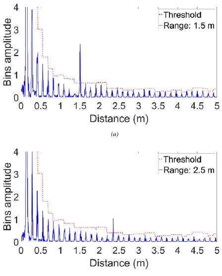
22 To the aim of evaluating the accuracy of the system, different tests have been performed. A metallic cylinder-shaped target (1.75 m height and 7.5 cm diameter) has been employed for performing two measurements at the distance of 1.5 m and 2.5 m. The IF data extracted from the microcontroller and the employed threshold have been reported in Fig. 1.13 for confirming the expected performance. More details about the threshold will be given in Section 1.5.

(a)

(b)

Fig. 1.13: IF signal (blue solid line) and threshold (red dashed line) for a target at (a) 1.5 m and (b) 2.5 m.

The distinctive feature of the present system is certainly the feasibility of being adapted to several short-range applications. This task can be accomplished by taking into consideration its compactness and cost-effectiveness, without affecting its performance. As a final step, a single board could be realized, thus reducing the overall dimensions.

23

1.4.3

Transmitter linearization

The frequency at the output of the BGT24MTR11 transmitter has been observed to be not linear with respect to the voltage-controlled oscillator’s tuning voltage [13]. This leads to a distorted IF signal at the output of the homodyne receiver that worsens the resolution of the radar, as shown in Fig. 1.14 for a target placed at 1.5 m. Ideally, a single target would generate an IF frequency spectrum composed by a single line. If the transmitter is nonlinear, the transmitted signal will contain more than one frequency harmonic and the frequency difference at the output of the mixer will generate a frequency spectrum composed by more than one line.

Fig. 1.14: Measured IF for a target placed at 1.5 m, without transmitter predistortion [14].

To the aim of improving the measurement accuracy, the following predistortion procedure has been implemented. The first step has been the measurement of the frequency of the transmitted signal for different tuning voltages by means of a spectrum analyzer (MXA9020A, Keysight Technologies) and an oscilloscope (TDS 2022B, Tektronix Inc.). Thereafter, the expression of the measured tuning voltage 𝑉𝑚, as a function of the measured frequency 𝐹𝑟𝑒𝑞𝑚, has been computed by using a fitting quadratic polynomial, reported in eq. (1.20):

𝑉_𝑚 = 0.165 ∙ 𝐹𝑟𝑒𝑞_𝑚2− 7.3791 ∙ 𝐹𝑟𝑒𝑞_𝑚+ 83.2749 (1.20)

where 𝐹𝑟𝑒𝑞_𝑚 is in GHz.

Equation (1.20) has been used for computing the tuning voltages required to achieve a frequency-linearized output, just replacing the term 𝐹𝑟𝑒𝑞𝑚 with a linearly-spaced set of frequencies. These values can be employed in place of the original ones by using the expression of the desired tuning voltage 𝑉_𝑙𝑖𝑛, as a function of the original measured ones. The required expression has been computed by using a fitting quadratic polynomial as shown in eq. (1.21):

24 𝑉_𝑙𝑖𝑛 = 0.3119 ∙ 𝑉_𝑡2− 0.0801 ∙ 𝑉_𝑡+ 0.8982 (1.21)

The above eq. (1.21) has been implemented into the microcontroller firmware for obtaining the desired output frequency whose trend vs time is illustrated in Fig. 1.15, showing evidence of the achieved relevant linearity improvements.

Fig. 1.15: Measured frequencies without (blue) and with (red) predistortion vs time [14].

Finally, the IF signal at the output of the homodyne receiver has been measured again with the same target placed at 1.5m. In Fig. 1.16 the IF signal is shown.

Fig. 1.16: Measured IF for a target placed at 1.5 m, with transmitter predistortion. [14].

The predistortion procedure allows the improvement of the measurement accuracy, thus enhancing the radar performance.

25

A novel approach for crosstalk minimization

Pointing towards high performance miniaturized circuitry, one of the main topics in a bidirectional communications system is the coexistence of a very sensitive receiver with a transmitter located in close proximity. The isolation between the components of the system has been extensively investigated by adopting either software or hardware techniques [15-18].

The adopted frequency-modulated radar architecture employs a homodyne receiver which typically is affected by crosstalk issue. This effect can severely worsen the radar performance because it overcomes the intermediate frequency beat and cannot be totally avoided. Otherwise, since it mainly appears in the lower bandwidth part of the IF signal, it could be reduced by means of two classical and well known methods. The first is based upon using a high-pass filter, the second discards the first FFT bins during the signal processing. Both these basic methods degrade the system performance, thus increasing the minimum detectable range. Some sophisticated solutions have been developed for the characterization and mitigation of crosstalk but they often employ expensive or heavy computational procedures and they are aimed at different applications [19-20].

The proposed method has been focused on the identification of the optimal threshold for detecting the target in presence of crosstalk, whose preliminary results are reported in [21]. In literature, it is common to find examples of radars employing an adaptive threshold, e.g., constant false alarm rate detectors. In these systems, the threshold is adjusted to the local interference level assuming that the noise level is homogeneous. By contrast, the present procedure takes in consideration that the cross-talk evolution is not casual. Indeed, once the radar architecture is defined, both the crosstalk and the signal at the output of the homodyne receiver decrease as the frequency increases [10]. Therefore, it is worthwhile employing a higher threshold in the low-frequency bandwidth than in the high-frequency one. For this reason, the first step of this approach has been the crosstalk mapping in absence of targets with the aim of performing a calibration of the receiver threshold. Thereafter, a suitable threshold for every sub-band has been identified according with the cross-talk level. This method aimed at overcoming the crosstalk effects offers two novel features: firstly, it does not require any alteration either in the radar mode of operation or in its hardware. Secondly, it can be employed in different radar applications because the procedure is independent of the architecture and it is not computationally heavy for the processing unit [14].

26 For evaluating the optimum threshold, the threshold values without any target have been collected. Although the crosstalk trend is quite steady with time, small oscillations of every IF peak have been observed. In order to take these variations in account, the threshold values have been collected over a period of 400 ms. The stored values, increased by a 10% margin, are employed to tailor the required threshold, which is shown in Fig. 1.17.

Fig. 1.17: Threshold (red) and IF signal without targets (red) [14].

In Fig. 1.18, the IF signal for a target at different distances has been reported. The system performance is very satisfactory both at shorter distances in presence of a higher crosstalk level, and at longer distances with lower echo strength. By using the proposed approach, the targets have been detected with a reduced computational effort and without discarding any bin.

27

(b)

(c)

Fig. 1.18: Threshold (red) and IF signal (black): (a) target at 0.5 m, (b) 1.5 m, (c) 3 m [14].

The presented approach has been found to be highly flexible for various radar scenarios, thus avoiding the typical restrictions due to the crosstalk noise.

A special application: a microwave white cane for visually

impaired people

As it is well known, people affected by blindness and visual diseases need to use special devices to overcome daily tasks, e.g. moving and navigating around unfamiliar environments. Usually, blind people walk assisted by supports ranging from the traditional white cane to more technological devices, namely Electronic Travel Aids (ETA) [22]. Such systems are mainly based on ultrasonic or optic sensors, whereas the use of the electromagnetic (EM) technologies to develop a support system for visually impaired people is a research topic currently under development [23].

28 It is generally agreed that neither ultrasonic nor optical ETA's satisfy all the needs of a visually impaired person. The ultrasonic ETA's exhibit a limited operating range due to problems when operating with highly reflective surfaces e.g. smooth surfaces, with a low incidence angle of the beam and when detecting small openings, e.g. a narrow door.

The optical ETA's do not suffer from similar drawbacks, but are affected by a high sensitivity to the natural ambient light or by the dependence on the optical characteristics of the target.

The most recent ETA devices employing an electromagnetic (EM) sensor have been proposed in [24, 25], both showing a 24 GHz frequency modulated continuous wave (FMCW) radar able to detect short-range targets.

In [24], the radar is shown to be successfully usable for different industrial and medical applications. One of these applications regards the possibility of augmenting the reality of visually impaired people by navigating through their daily lives. It is proposed that a radar sensor scans the environment, then the target angle and distance information are collected, evaluated and mapped into the audio space by using virtual 3D audio rendering techniques. A FMCW radar has been used in [25] with the aim of realizing a device to be mounted on a white cane. Great attention has been paid to the antenna design, but no details on the system performances nor evidence of proofs with actual end users have been reported.

In this context, our preliminary studies had previously concerned the comparison between the performances of an EM system and those of the traditional supports [26]. This type of investigation had never been presented in the literature, thus representing a pioneer research activity on the expected advantages coming from the adoption of the EM technology as an aid for visually impaired users. Briefly, such preliminary investigations demonstrated the potential for the EM technology in terms of resolution, efficiency and comfort for the user. Since the very first tests were carried out by using laboratory instrumentation, hereby the attention has been focused on the realization of a cost-effective compact radar system characterized by a suitable performance.

The main idea is to realize a device small enough to be attached onto the white cane to enhance the usefulness of a traditional and widely accepted travel aid [27, 9]. As a matter of fact, when realizing a novel support for disable people, it is important not to forget the personal considerations and impressions of end users. The positive reception of a new device within the blind community is a very critical issue. Most requirements concern aesthetics characteristics and appearance: they should be unobtrusive, unnoticeable and easy to carry [28]. For such

29 reasons a small and user-friendly component integrated onto the white cane, the most widely used and accepted system, has been designed in order to make the user more confident and eager to try the new technology.

As stated above, two microwave antennas have been designed, realized and characterized in collaboration with the Department of Information Engineering, Università Politecnica delle Marche.

The system works as a short-range radar and has to satisfy the following requirements, arising from the specific and innovative type of application:

1. small dimensions and reduced weight, to preserve the user’s comfort and to promote the acceptability of a new device;

2. working frequency inside the free-use band for short-range radar applications as defined by the national and international regulations [29]. A resolution of about 10-20 cm is required, which implies a frequency bandwidth of about 1 GHz;

3. radiation pattern shaped as a vertical fan beam, narrow over the horizontal plane (≤ 10°) and wide over the vertical one (about 40°), as schematically depicted in Fig. 1.19. Over the azimuthal plane, the direction of the obstacle is detected by scanning the environment with the classical horizontal motion of the cane. This scenario has been described in Fig. 1.19a. Over the elevation plane, as shown in Fig. 1.19b, the wide beam allows even the detection of suspended obstacles, e.g. the branch of a tree;

4. observation range from 1 m to 5 m. Such limits have been arbitrarily chosen according to the end user needs. Indeed, the radar is designed to be mounted on the white cane, which efficiently works for very short distances (< 1 m). The upper limit of 5 m is a tradeoff between the need to efficiently warn the user about the presence of obstacles, and the risk of annoying him with warnings due to very far targets. The system is able of generating a maximum output power of 11 dBm. This value complies with the international regulations regarding the exposure to EM fields [30]. Accordingly, at a distance of 1 m from the antenna (a reasonable minimum distance considering the presence of the white cane) the regulation imposes a maximum E field of 6 V/m, which in this case corresponds to a maximum power of 15 dBm.

30 (a)

(b)

Fig. 1.19: Schematic representation of the EM beam shape due the radar mounted onto a white cane showing (a) top and (b) lateral view [12].

In Fig. 1.20, a picture of the final laboratory prototype, including the radar architecture, the two antennas and all the RF connections, is shown.

Fig. 1.20: Picture of the radar system including the prototyping board, the MCU board and the two microwave antennas [12].

In order to define the minimum detectable signal, a preliminary measurement without targets has been performed. The poor isolation between transmitter and receiver leads to the crosstalk

31 noise level, clearly visible in Fig. 1.21. In order to account for this noise level, and hence for the minimum detectable signal, a threshold has been set at twice the level of the crosstalk noise (in order to guarantee a guard level), as highlighted in Fig. 1.21. Each signal measured by the radar system is normalized to the maximum value of such noise and each echo larger than the noise threshold is associated to an obstacle.

Fig. 1.21: Crosstalk noise caused by the finite isolation between the transmitter and the receiver (blue line) and threshold level (yellow line) [12].

Then, several measurements have been carried out in order to verify the system performance in a real environment, by locating the radar at the height of 1 m from the ground since this is expected to be the final position on the white cane handle.

A cylindric metallic target (1.75 m height and 7.5 cm diameter) has been placed at increasing distances from the radar, ranging from 0.5 m to 3.5 m, as shown in Fig. 1.22. Despite the design requirement, the upper limit is currently limited to 3.5 m because of two main reasons: losses in the microwave connections (around 2 dB) and missing amplification stage at the intermediate frequency in the receiver chain (it will be added to the final prototype).

32

Fig. 1.22: IF signals for target distances from 0.5 to 3.5 m and threshold (yellow line). [12].

Another set of measurements has been performed for confirming the radar capability of detecting targets with a very high horizontal selectivity. The FFT data related to the IF frequency signal have been extracted from the MCU memory. In Fig. 1.23 such data are reported for different angular positions of the target over the horizontal plane, together with the corresponding value of the threshold noise. The same cylindric reflecting obstacle used in the previous tests and located at a distance of 1.5 m from the radar has been used. It is seen that the target can be correctly detected within an angular sector of +/- 3° with respect to the main lobe position, whereas it is almost undetectable at +/- 7° where the signal level is masked by the cross-talk noise. These results confirm the high spatial selectivity of the system.

33 Afterwards, the capability of detecting obstacles suspended at different heights with respect to the radar has been tested. The radar has been located one meter above the ground whereas the cylindric obstacle has been moved along different vertical angular positions, according with the design requirements defined in Section II.

Indeed, since using the bare white cane typically allows detection of obstacles lying on (or close to) the ground, it is extremely important to design a device able to protect the user against collisions with obstacles located at different elevations. Once again, a very good performance of the system has been observed since the radar has proven its ability to detect the presence of a suspended obstacle, according to the aperture of the TX radiation pattern. Indeed, the vertical location of the target can be correctly detected within an angular sector of +/- 17°. The related measurement results are shown in Fig. 1.24.

Fig. 1.24: IF signal for target vertical angular position of 0°, +/-17° and +/-36° [12].

The total beam of the radar system is due to the combination of both the TX and the RX radiation patterns. The results presented in Figs. 1.23-1.24 demonstrate that both antennas have been efficiently designed and optimized, because the requirements on azimuthal and elevation apertures are fully satisfied.

Finally, the system capability of detecting obstacles of different shapes, dimensions and materials has been tested, as a preliminary demonstration of the usefulness of such system for daily tasks. In particular, a wooden chair, a chest of drawers and a human subject have been considered. All of them, located at the distance of 1.5 m from the radar have shown to be easily

34 detectable, since their echoes are sensibly greater than the noise threshold, as shown in Fig. 1.25.

Fig. 1.25: Radar signals for different obstacles located at 1.5 m. From the top to the bottom, a human target, a chest of drawers and a wooden chair are detected [12].

In the case of the chair, the margin with respect to the noise threshold is low. In the final version of the prototype, this aspect will be taken into consideration for obtaining a better signal-to-noise ratio, thus allowing the detection of targets in a wider range.

The topics treated above have been detailed and presented in a paper submitted for publication in Sept. 2017 [12].

References

[1] M. A. Richards, J. A. Scheer, W. A. Holm, “Principles of Modern Radar: Basic principles,” SciTech Publishing, 2010.

[2] W. L. Melvin, J. A. Scheer, W. A. Holm, “Principles of Modern Radar: Radar applications,” SciTech Publishing, 2014.

[3] Caputi Jr., W.J., “Stretch: A Time-Transformation Technique,” IEEE Trans. on Aerosp.

and Electr. Sys., Vol. AES7, Mar. 1971.

35 [5] M. I. Skolnik, “Radar Handbook,” 2nd ed., Ed., McGraw-Hill Co., 1990.

[6] Vizmuller, P., “RF Design Guide: Systems, Circuits and Equations,” Artech House, Inc., 1995.

[7] Richards, M.A., “Fundamentals of Radar Signal Processing,” McGraw-Hill, 2005. [8] Kay, S.M., “Fundamentals of Statistical Signal Processing. Vol. II: Detection Theory,”

Prentice-Hall, 1998.

[9] V. Di Mattia, G. Manfredi, A. De Leo, P. Russo, L. Scalise, G. Cerri, A. Caddemi, and E. Cardillo, “A Feasibility Study of a Compact Radar System for Autonomous Walking of Blind People,” 2016 IEEE 2nd International Forum on Research and Technologies for

Society and Industry Leveraging a better tomorrow (RTSI), Bologna, Sept. 2016.

[10] Infineon BGT24MTR11 datasheet, Rev. 3.1, 2014. [11] Infineon XMC4500 datasheet, V1.4 2016-01.

[12] E. Cardillo, V. Di Mattia, G. Manfredi, P. Russo, A. De Leo, A. Caddemi, and G. Cerri, “An electromagnetic sensor prototype to assist visually impaired and blind people in autonomous walking,” IEEE Sensors J., Mar. 2018.

[13] Infineon App. Note AN305, User’s guide to BGT24MTR11 24 GHz Radar, rev. 1.0, 2012 [14] E. Cardillo, and A. Caddemi, “A novel approach for crosstalk minimization in FMCW

radars,” Electronics Lett., Sept. 2017.

[15] M. Guenach, J. Louveaux, L. Vandendorpe, P. Whiting, J. Maes, and Mi. Peeters, “On signal-to-noise ratio-assisted crosstalk channel estimation in downstream DSL systems,”

IEEE Trans. Signal Process., vol. 58, Apr. 2010.

[16] S. A. Bassam, M. Helaoui, and F. M. Ghannouchi, “Crossover digital predistorter for the compensation of crosstalk and nonlinearity in MIMO transmitters,” IEEE Trans. Microw.

Theory Techn., Vol. 57, May. 2009.

[17] N. Al-Dhahir, “Transmitter optimization for noisy ISI channels in the presence of crosstalk,” IEEE Trans. Signal Process., vol. 48, Apr. 2000.

36 [18] A. Hjørungnes, M. L. R. de Campos, and P. S. R. Diniz, “Jointly optimized transmitter and receiver FIR MIMO filters in the presence of near-end crosstalk,” IEEE Trans. Signal

Process., vol. 53, Apr. 2005.

[19] C. Trampuz, I. E. Lager, M. Simeoni, and L. P. Ligthart, “Experimental characterization of channel crosstalk in interleaved array antennas for FMCW radar,” Proc. 7th _European Radar Conference - EuRAD, Paris, Oct. 2010.

[20] H. Tan, and J. Hong, “Correction of transmit crosstalk in reconstruction of quad-pol data from compact polarimetry data,” IEEE Trans. Geosci. Remote Sens., vol. 12, May. 2015. [21] Caddemi, and E. Cardillo, “A study on dynamic threshold for the crosstalk reduction in frequency-modulated radars,” Computing and Electromagnetics International Workshop

(CEM), Barcelona, Jun. 2017.

[22] D. Dakopoulos and N. G. Bourbakis, “Wearable Obstacle Avoidance Electronic Travel Aids for Blind: A Survey,” IEEE Trans. on systems, man, and cybernetics—Part c:

Applications and reviews, vol. 40, Jul. 2010.

[23] V. Di Mattia, L. Scalise, V. Petrini, P. Russo, A. De Leo, E. Pallotta, A. Mancini, P. Zingaretti And G. Cerri, "Electromagnetic technology for a new class of electronic travel aids supporting the autonomous mobility of visually impaired people", Chapter Book Entitled "Visually Impaired: Assistive Technologies, Challenges And Coping Strategies" Nova Science Publishers, Inc. 2016.

[24] S. Jardak, T. Kiuru, M. Metso, P. Pursula, J. Häkli, M. Hirvonen, S. Ahmed, M. Alouini "Detection and localization of multiple short range targets using FMCW radar signal,"

2016 Global Symposium on Millimeter Waves (GSMM) & ESA Workshop on Millimetre-Wave Technology and Applications, Espoo, 2016.

[25] S. Pisa, E. Pittella, and E. Piuzzi, “Serial Patch Array Antenna for an FMCW Radar Housed in a White Cane,” International Journal of Antennas and Propagation, vol. 2016, Article ID 9458609, 2016.

[26] L. Scalise, V. Primiani, P. Russo, D. Shauh, V. Di Mattia, A. De Leo, G. Cerri “Experimental investigation of electromagnetic obstacle detection for visually impaired

37 users: a comparison with ultrasonic system”, IEEE Trans. Instrum. Meas., vol. 61, Nov. 2012.

[27] V. Di Mattia, V. Petrini, M. Pieralisi, G. Manfredi, A. De Leo, P. Russo, L. Scalise, G. Cerri. “A K-band miniaturized antenna for safe mobility of visually impaired people,”

IEEE 15th Mediterranean Microwave Symposium (MMS), Lecce 2015.

[28] Hersh, Marion and Johnson, Michael A., Assistive Technology for Visually Impaired and Blind People, Springer-Verlag, London 2008.

[29] Commission Implementing Regulation (EU) No 485/2011 of 18 May 2011, Official Journal of the European Union 133, 20.5.2011.

38

2 Noise in radar receivers

This Chapter begins by describing the origin of noise and its importance in radar receivers. Thereafter, a complete analysis of noise in radar receivers is carried out starting from the basic element, the transistor, to the key component, the LNA. Moreover, both the behavior of the transistor and the LNA are deeply analyzed under light exposure since a part of the research work has been dedicated to this aspect. In addition, a low-noise amplifier has been designed, realized and tested under standard and light conditions.

Noise

As described in the previous Chapter, the receiver is a critical section of a radar system, as its basic function is to distinguish between signal and noise. The noise is critical for the radar performance because it determines the minimum signal that can be detected. The noise internally generated by a component or by an electron device is produced by the random motion of charges in the material. It can be due to different physical mechanisms, thus leading to various types of noise [1], [2]:

 Thermal, Johnson or Nyquist noise, due to thermal vibration of bound charges.  Shot noise, due to random fluctuations of charge carriers in an electron tube or

solid-state device.

 Flicker or 1/f noise, occurs in an electron tube or solid-state device and its power is inversely proportional to the frequency.

 Plasma noise, due to the random motion of charges in an ionized gas.  Quantum noise, due to the quantized nature of charge carriers and photons.

The noise produced by a system can be characterized in terms of its noise figure. This parameter was introduced by Harald T. Friis of Bell Laboratories who defined the noise figure F of a network as a measure of the degradation in the signal-to-noise ratio (SNR) occurring between the input and the output network ports [3]. By applying a signal affected by noise to the input of a noiseless network, both the noise and the signal will be amplified or attenuated in the same way, thus the SNR will not change. In the case of a noisy network, the output noise

39 power will increase more than the signal power, thus reducing the SNR. For measuring this degradation, the noise figure, F is defined as in eq. (2.1):

𝐹 = 𝑆_𝑖 𝑁_𝑖 ⁄ 𝑆𝑜 𝑁𝑜 ⁄ ≥ 1 (2.1)

where 𝑆_𝑖 and 𝑁_𝑖 are the input available signal and noise powers, respectively, whereas 𝑆_𝑜 and 𝑁_𝑜 are the output available signal and noise powers, respectively. Bearing in mind that the available noise power of a resistor at 𝑇0 = 290 𝐾 is expressed as in eq. (2.2):

𝑁_𝑖 = 𝑘𝑇₀𝐵 (2.2)

and considering the circuit shown in Fig. 2.1, referred to a noisy network with a gain (G), a bandwidth (B) and an equivalent noise temperature 𝑇𝑒, the noise figure is given by eq. (2.3):

𝐹 = 𝑆𝑖 𝑘𝑇₀𝐵 𝑘𝐺𝐵(𝑇0+ 𝑇𝑒) 𝐺𝑆_𝑖 = 1 + 𝑇𝑒 𝑇₀ ≥ 1 (2.3)

Fig. 2.1: Noisy network [1].

In a typical radar receiver, the received echo passes throughout a series of different stages, each one modifying the signal itself. Given the noise figure and the gain of each stage, it is possible to derive the overall noise figure of the system 𝐹_𝑠𝑦𝑠 by using eq. (2.4):

𝐹_𝑠𝑦𝑠 = 𝐹₁+𝐹2− 1 𝐺₁ +

𝐹3− 1 𝐺₁𝐺₂ + ⋯

40 Since 𝐹_𝑖 is the noise figure of the ì-th stage, a clear consequence of eq. (2.4) is that the overall noise figure of the system mainly depends on the first stage. For this reason, usually the LNA is employed as the first active stage of a radar receiver, to amplify the very weak received signal with a minimum additional noise. Besides, passive stages standing between the receiving antenna and the LNA are to be avoided, as much as possible, since their losses (under thermal equilibrium conditions) translate into an additional noise figure value directly added to the chain.

Noise in microwave transistors

Before analyzing in detail the LNA characteristics, it is worth having a deep insight into the LNA structure. In the following, the active device of the LNA, i.e. the transistor employed, will be analyzed with a special concern to its noise behavior.

In the previous paragraph, the analyzed network has been supposed to be matched to the characteristic impedance at both input and output ports. On the contrary, the typical situation of a microwave transistor within a microwave amplifier is that of a deeply mismatched device, leading to a substantial difference in complexity when compared with the noise performance of a matched one. The noisy network in Fig. 2.1 can be transformed into the network in Fig. 2.2, in which |𝑖̅̅̅̅̅𝑠|2 is the mean squared value of the noise current due to the noise source, 𝑌𝑆 is the source admittance, 𝑒_𝑛 and 𝑖_𝑛 are the noise sources to be treated as stochastic signals, correlated by means of a complex correlation coefficient.

41 As it can be easily demonstrated, the noise figure can be computed by using the expression reported in eq. (2.4),[4]: 𝐹 = |i𝑡𝑜𝑡| 2 ̅̅̅̅̅̅̅̅ |i𝑠|2 ̅̅̅̅̅ (2.4)

where |i̅̅̅̅̅̅̅̅ is the mean squared value of the noise current evaluated at the output of the 𝑡𝑜𝑡|2 network with short-circuited terminals.

In real transistors the noise sources are generally correlated, thus a value of source impedance for creating the condition of minimum noise figure exists for each frequency. This concept is essential for understanding the noise parameters. Although these physical noise generators produce noise in both the forward and reverse directions, transistors have gain in one direction, but losses in the other. As a result, the magnitude and phase change in each direction. If there is correlation between the noise sources, then there will be some value of source impedance (Γ_𝑜𝑝𝑡 in eq. (2.5)) that provides the right amount of magnitude and phase shift to cause maximum cancellation, which results in a minimum noise figure.

Finally, it is possible to extract the well-known expression of eq. (2.5) [4]:

𝐹 = 𝐹_𝑚𝑖𝑛+ 4𝑅𝑛 𝑍₀ |Γ_𝑠− Γ_𝑜𝑝𝑡|2 |1 − Γ_𝑜𝑝𝑡|2(1 − |Γ_𝑠|2₎ (2.5) where:

𝐹_𝑚𝑖𝑛 is the minimum noise figure, occurring when Γ_𝑠 = Γ_𝑜𝑝𝑡 .

𝑅_𝑛 is the noise resistance and represents how fast 𝐹 degrades as Γ_𝑠 moves away from Γ_𝑜𝑝𝑡. 𝑍0 is the characteristic impedance, usually 50 Ω.

Γ_𝑠 is the source reflection coefficient.

Γ_𝑜𝑝𝑡 is the optimum noise reflection coefficient, i.e. the value of Γ_𝑠 that allows to obtain the minimum noise figure.

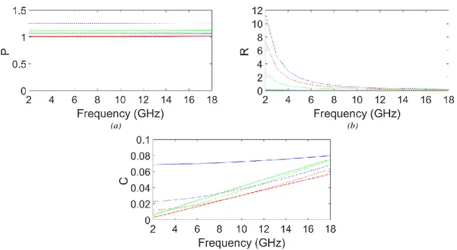
The so-called four noise parameters (N-parameters) are 𝐹_𝑚𝑖𝑛, magnitude and phase of Γ_𝑜𝑝𝑡, and 𝑅_𝑛 [5]. Their knowledge is of basic importance when designing a low-noise amplifier based on highly mismatched devices. They are usually furnished by the manufacturer in the data sheet of the transistor or they can be experimentally determined. A LNA design involves a trade-off between gain, noise figure, VSWR and frequency behavior. The noise parameters strongly depends on the frequency and operating conditions and they can be represented graphically in

42 different forms [6]. By using a 3-D parabolic-like surface, the role played by each noise parameter can be better understood. A Matlab® script has been used for representing the parabolic-like surface changing different parameters. In Fig. 2.3, a noise surface at a fixed frequency for different values of 𝑅_𝑛 has been represented, showing that the aperture of the surface decreases as its values increase.

(a) (b)

(c)

Fig. 2.3: Noise surface for different values of 𝑅𝑛: (a) 5 Ω, (b) 20 Ω, (c) 80 Ω.

In Fig. 2.4, a noise surface at a fixed frequency for different values of 𝐹_𝑚𝑖𝑛 has been represented. The minimum height increases together with the 𝐹𝑚𝑖𝑛 values.

43

(a) (b)

(c)

Fig. 2.4: Noise surface for different values of 𝐹𝑚𝑖𝑛: (a) 1 dB, (b) 2 dB, (c) 3 dB.

The procedure for extracting the noise parameters is very complex, in terms of both data processing and hardware set-up, and time-consuming as well. The noise figure of the device under test’s (DUT) is masked by the contribution of the measurement chain and the overall accuracy is affected by several factors. The two mainly used measurement techniques are the Y-factor (hot/cold source) and the cold source (direct noise), but the former is predominant especially in commercial systems.

The Y-factor method essentially uses a calibrated noise source that can be turned on and off. A noise figure meter measures the output power in these two states. This amount of extra noise between the on (hot) and off (cold) state is called excess noise ratio (ENR). Typical ENR values vary from 5 dB to 15 dB. After the noise power measurement, the noise figure of the entire system can be computed following the steps reported from eq. (2.6) to eq. (2.9):