Jets in Hydrogen-poor Superluminous Supernovae: Constraints from a Comprehensive
Analysis of Radio Observations
D. L. Coppejans1 , R. Margutti1 , C. Guidorzi2 , L. Chomiuk3 , K. D. Alexander4 , E. Berger4 , M. F. Bietenholz5,6 , P. K. Blanchard4, P. Challis4, R. Chornock7, M. Drout8, W. Fong1,13 , A. MacFadyen9 , G. Migliori10 , D. Milisavljevic11 ,
M. Nicholl4 , J. T. Parrent4 , G. Terreran1, and B. A. Zauderer9,12 1
Center for Interdisciplinary Exploration and Research in Astrophysics(CIERA) and Department of Physics and Astronomy, Northwestern University, Evanston, IL 60208, USA
2
Department of Physics and Earth Science, University of Ferrara, via Saragat 1, I-44122, Ferrara, Italy 3
Department of Physics and Astronomy, Michigan State University, East Lansing, MI 48824, USA 4
Harvard-Smithsonian Center for Astrophysics, 60 Garden St., Cambridge, MA 02138, USA 5
Hartebeesthoek Radio Observatory, P.O. Box 443, Krugersdorp, 1740, South Africa 6
Department of Physics and Astronomy, York University, Toronto, M3J 1P3, ON, Canada 7
Astrophysical Institute, Department of Physics and Astronomy, 251B Clippinger Lab, Ohio University, Athens, OH 45701, USA 8
Carnegie Observatories, 813 Santa Barbara Street, Pasadena, CA 91101, USA 9
Center for Cosmology and Particle Physics, New York University, 4 Washington Place, New York, NY 10003, USA 10
Laboratoire AIM(CEA/IRFU—CNRS/INSU—Université Paris Diderot), CEA DSM/IRFU/DAp, F-91191 Gif-sur-Yvette, France 11Department of Physics & Astronomy, Purdue University, West Lafayette, IN 47907, USA
12
National Science Foundation, 2415 Eisenhower Avenue, Alexandria, VA 22314, USA
Received 2017 November 8; revised 2018 February 2; accepted 2018 February 26; published 2018 March 26
Abstract
The energy source powering the extreme optical luminosity of hydrogen-stripped superluminous supernovae (SLSNe-I) is not known, but recent studies have highlighted the case for a central engine. Radio and/or X-ray observations are best placed to track the fastest ejecta and probe the presence of outflows from a central engine. We compile all the published radio observations of SLSNe-I to date and present three new observations of two new SLSNe-I. None were detected. Through modeling the radio emission, we constrain the subparsec environments and possible outflows in SLSNe-I. In this sample, we rule out on-axis collimated relativistic jets of the kind detected in gamma-ray bursts (GRBs). We constrain off-axis jets with opening angles of 5° (30°) to energies of
Ek<4´1050erg (Ek<1050erg) in environments shaped by progenitors with mass-loss rates of M <10-4M yr-1
˙ (M <10-5M yr-1
˙ ) for all off-axis angles, assuming fiducial values e=0.1 and
0.01 B
= . The deepest limits rule out emission of the kind seen in faint uncollimated GRBs (with the exception of GRB 060218) and from relativistic SNe. Finally, for the closest SLSN-I, SN 2017egm, we constrain the energy of an uncollimated nonrelativistic outflow like those observed in normal SNe to Ek1048erg. Key words: stars: jets– supernovae: general
1. Introduction
Superluminous supernovae (SLSNe) are a distinct class of
supernovae (SNe) that have UV-optical luminosities
L >7 ´1043erg s-1 (Chomiuk et al. 2011; Quimby et al.
2011). These stellar explosions are typically ∼10–100 times
more luminous than ordinary SNe,14 show comparatively bright UV emission at early times, and, in some cases, have decay rates that are incompatible with 56Ni and 56Co decay (Gal-Yam2012; De Cia et al.2017; Lunnan et al.2018).
There are two main classes of SLSNe, namely, the hydrogen-rich systems (SLSNe-II) and the hydrogen-stripped systems (SLSNe-I). Some SLSNe-II show clear signatures of shock interaction with a dense medium in their optical spectra (in the form of narrow emission lines with width 100 km s< -1).
For these systems, the large UV-optical luminosity can be explained through the interaction of the blast wave with dense material left behind by the stellar progenitor before collapse (e.g., Ofek et al. 2007; Smith & McCray2007; Chatzopoulos et al. 2011). The mechanism or mechanisms that power the
exceptional luminosities of SLSNe-I, however, are unknown (e.g., Gal-Yam2012).
A number of models for the energy source of SLSNe-I have been proposed. Higher luminosities could be explained by the presence of larger quantities of radioactive material (with respect to ordinary SNe) or a central engine. Large quantities of 56Ni could be produced by a pair-instability SN (Woosley et al.2007; Gal-Yam et al.2009). A central engine in the form
of the spindown of a magnetar (e.g., Kasen & Bildsten2010; Woosley 2010; Nicholl et al. 2013; Metzger et al. 2015) or
fallback accretion onto the compact remnant (Dexter & Kasen 2013) has been suggested. The source of the large
luminosity could also be due to increased efficiency of the conversion of kinetic energy into radiation via shock interac-tion in a particularly dense circumstellar medium(e.g., Smith & McCray 2007; Chevalier & Irwin 2011; Ginzburg & Balberg2012).
The mechanism(or mechanisms) powering the luminosity of SLSNe-I are a topic of debate. A key problem with the interaction model is that no clear evidence for a dense surrounding medium (such as narrow spectral lines with v100 km s−1 at early times) has been observed in SLSNe-I. Roth et al. (2016), however, showed that under the right
conditions, the narrow-line emission could be suppressed. Hα © 2018. The American Astronomical Society. All rights reserved.
13
Hubble Fellow. 14
Note that Milisavljevic et al.(2013) and Lunnan et al. (2018) found SNe
emission has been detected at late times in three SLSNe-I(Yan et al. 2015, 2017a): to power this emission and not produce
narrow lines, a few solar masses of hydrogen-free material would need to have been ejected in the last∼year before stellar explosion (e.g., Chevalier & Irwin 2011; Chatzopoulos & Wheeler2012; Ginzburg & Balberg2012; Moriya et al.2013).
There are, however, claims that interaction of the ejecta with the medium is necessary to fit the light curves of some SLSNe-I, regardless of whether interaction is the dominant contribution to theflux (e.g., Yan et al.2015; Wang et al.2016; Tolstov et al. 2017).
Pair-instability SNe (Barkat et al.1967) could produce the
required amounts of 56Ni to power the optical luminosity, but to date, only two candidates are known(Gal-Yam et al.2009; Terreran et al. 2017), and the classification is debated in the
literature(e.g., Yoshida & Umeda2011; Nicholl et al.2013). If
the radioactive decay of56Ni is the sole energy source, then for some SLSNe-I, the necessary quantities cannot be reconciled with the inferred ejecta mass, bright UV emission, or decay rate of the light curves(e.g., Kasen et al.2011; Dessart et al.2012; Inserra et al. 2013; Nicholl et al.2013; McCrum et al. 2014; see, however, Kozyreva et al.2017). Pair-instability explosions
cannot account for the entire class of SLSNe-I.
Recent studies are increasingly favoring the central engine model(e.g., Margalit et al.2018; Nicholl et al.2017c), as it has
been shown to satisfactorily reproduce the optical light curves of SLSNe-I with a wide range of properties(e.g., Chatzopoulos et al. 2013; Inserra et al. 2013; Nicholl et al. 2014, 2017b; Metzger et al. 2015; Inserra et al. 2017). Magnetar central
engines with initial spin periods in the range 1–5 ms and magnetic fields in the range ≈1013–1014G are the bestfit for the optical bolometric emission of several systems (e.g., Dessart et al. 2012; Inserra et al. 2013; Nicholl et al. 2013; Metzger et al.2015; Lunnan et al. 2016; Yu & Li2017).
There is growing evidence of a link between jetted long gamma-ray burst (GRB) SNe and SLSNe-I in the form of observational similarities in their spectra and light curves(e.g., Greiner et al. 2015; Metzger et al. 2015; Kann et al. 2016; Nicholl et al.2016a; Jerkstrand et al.2017), their preference for
metal-poor host galaxies(e.g., Lunnan et al.2014; Chen et al.
2015, 2017a, 2017c; Perley et al.2016; Izzo et al. 2018; but also see Bose et al. 2018; Chen et al. 2017b; Nicholl et al. 2017a),15 and the models for the central engine (e.g., Metzger et al. 2015; Margalit et al. 2018). SLSNe and GRB
SNe have broader spectral features than normal H-stripped SNe indicative of large photospheric velocities (Liu et al. 2017).
Additionally, the luminous UV emission in the SLSN-I Gaia16apd has been suggested to originate from a central engine(Nicholl et al.2017b; see, however, Yan et al.2017b).
In the SLSN-I SCP06F6, luminous X-ray emission(outshining even GRBs at a similar post-explosion time by a large factor), if indeed associated with the transient, is likely powered by a central engine (Gänsicke et al. 2009; Levan et al. 2013; Metzger et al.2015). The presence of a central engine may also
provide an additional driving force for the stellar explosion (e.g., Liu et al. 2017; Soker & Gilkis2017).
A key manifestation of a central engine is an associated jet. The search for evidence of a jet is best conducted at radio and X-ray wavelengths. Optical emission is of thermal origin and tracks the slowly moving material in the explosion(va few
10 km s4 -1). In contrast, radio and X-ray emission are of
nonthermal origin and arise from the interaction of the explosion’s fastest ejecta (v0.1c) with the local
environ-ment. As the radiative properties of the shock front are directly dependent on the circumstellar density, radio/X-ray observa-tions also probe the mass-loss history of the progenitor star in the years prior to explosion, a phase in stellar evolution that is poorly understood(see Smith2014for a recent review).
In Margutti et al. (2017a), we used the sample of X-ray
observations of SLSNe-I to constrain relativistic hydrodyna-mical jet models and determine constraints on the central engines and subparsec environments of SLSNe-I. This work showed that interaction with a dense circumstellar medium is not likely to play a key role in powering SLSNe-I, and that at least some SLSN-I progenitors are compact stars surrounded by a low-density environment. There was no compelling evidence for relativistic outflows, but the limits were not sensitive enough to probe jets that were pointed more than 30° out of our line of sight. In one case (PTF12dam), the X-ray limits were sufficiently deep to rule out emission similar to subenergetic GRBs, suggesting a similarity to the relativistic SNe 2009bb and 2012ap (Soderberg et al. 2010b; Margutti et al. 2014; Chakraborti et al. 2015) if this SLSN-I was a jet-driven
explosion.
In this paper, we expand on recent analysis of radio observations from the SLSN 2015bn (Nicholl et al. 2016a; Margalit et al. 2018) and compile all the radio-observed
SLSNe-I, including the three new observations presented for the first time in this work, with the aim of placing stronger constraints on the properties of their subparsec environment and fastest ejecta(both in the form of a relativistic jet and an uncollimated outflow). These data span ∼26–318 days after the explosion(in the explosion rest frame and at GHz frequencies). We test for the presence of a central engine that would produce a GRB-like jet and model the on-axis and off-axis emission from a jet for a range of densities, microphysical shock parameters, kinetic energies, jet opening angles, and off-axis observer angles and compare these to observations. We also explore the radio properties of uncollimated outflows that would be consistent with our limits and derive constraints on the fastest ejecta and mass-loss history of SLSNe-I.
In Section 2, we describe the sample of radio-observed SLSNe-I. In Section3, we present our new radio observations of SLSNe-I and provide details on the data reduction. The constraints on on-axis and off-axis jets are given in Section4. Section5 describes the constraints we derive for uncollimated outflows. Conclusions are drawn in Section6.
Unless otherwise stated, all time intervals and frequencies are quoted in the explosion rest frame, and the error bars are
1σ. We assume a Λ cold dark matter cosmology with
H0=70 km s−1Mpc−1(h=0.7), Ω0=0.3, and ΩΛ=0.7. 2. Sample
Our sample consists of all H-stripped SLSNe with published radio observations as of 2017 August, comprising nine SLSNe-I. This includes seven systems with radio observations already published in the literature (PS1-10ky, PS1-10awh, PS1-12fo, iPTF15cyk, SN 2015bn, PTF09cnd, and SN 2017egm) and two systems (PS1-10bzj and Gaia16apd) for which we present the first radio observations. We also present the latest observations of SN 2017egm, updating the observations from Bose et al. (2018). A brief description of each SLSN is given in the
15
See Lunnan et al.(2014), Leloudas et al. (2015), Angus et al. (2016), and
Appendix. Table 1 gives the radio observations and relevant references for all of these systems.
The exact date of explosion is not known for every object in this sample. In a number of cases, the times of the observations (in number of days since the explosion) were derived from the time of peak luminosity and an estimated rise time. Given the spread in rise times for SLSNe-I (see Nicholl et al. 2017c), the uncertainty on these derived
observation times is less than 20 days. We tested the impact
of this uncertainty on our conclusions in the following analysis by increasing and then decreasing the assumed rise times of all objects in our sample by 20 days. The differences in the constraints that we derive are marginal and do not affect our conclusions.
3. Observations
Our observations of SN 2017egm (NRAO observing code VLA/17A-466; PI: R. Margutti), Gaia16apd (VLA/16A-476; Table 1
Properties of the Sample of SLSNe-I Name(s) dL Explosion Date Time After Expl.
a
Freq.a Specific Luminosity References
(Mpc) (MJD) (days) (GHz) (erg/s/Hz) PTF09cnd 1306b 55006c 85 10.6 <1.5×1029 Chandra et al.(2009b) 85 6.1 <1.6×1029 Chandra et al.(2009b) 85 1.8 <9.4×1031d Chandra et al.(2009b) 140 10.6 <1.1×1029 Chandra et al.(2010) 142 6.1 <2.4×1029 Chandra et al.(2010) 147 1.8 <9.7×1029d Chandra et al.(2010)
PS1-10awh 5865 55467 39 9.6 <9.7×1029 Chomiuk et al.(2011)
PS1-10bzj 3891e 55523e 48 8.2 <8.6×1029 This work
PS1-10ky 6265 55299f 156 9.6 <1.2×1030 Chomiuk et al.(2011)
SN 2012ilg 825h 55919i 44 6.9 <1.5×1028 Chomiuk et al.(2012a)
SN 2015bnj 528 57013k 318 8.2 <2.2×1028 Nicholl et al.(2016b)
318 24.5 <1.2×1028d Nicholl et al.(2016b)
iPTF15cyk 3101l 57249m 61 8.3 <2.2×1029 Palliyaguru et al.(2016), Kasliwal et al. (2016)
94 8.3 <1.7×1029 Palliyaguru et al.(2016), Kasliwal et al. (2016)
124 8.3 <1.7×1029 Palliyaguru et al.(2016), Kasliwal et al. (2016)
Gaia16apdn 467o 57512p 26 6.6 <4.7×1027 This work
26 24.0 <1.1×1028d This work
203 6.6 <3.6×1027 This work
203 24.0 <7.6×1027d This work SN 2017egmq 136r 57887s 34 16.0 <3.9×1028d,t Bright et al.(2017)
38 5.2 <1.3×1027d Bright et al.(2017)
39 10.3 <5.7×1026,u Romero-Canizales et al.(2017), Bose et al. (2018) 39 1.6 <2.1×1027d Romero-Canizales et al.(2017), Bose et al. (2018)
46 34.0 <3.3×1027d This work; Coppejans et al.(2017)
47 10.3 <6.4×1026,u Romero-Canizales et al.(2017), Bose et al. (2018) 74 34.0 <7.4×1026d This work
Notes.3σ upper limits are given on the luminosity. a
Explosion rest frame. b
Neill et al.(2011).
c
From Quimby et al.(2011), the peak time is MJD 55069.145 and assuming a rest-frame rise time of 50 days.
d
Not used in the modeling of emission from off-axis jets(Section4), because the explosion rest-frame frequency is significantly different from ∼8 GHz.
e
The peak was at MJD 55563.65+−2 (Lunnan et al.2013), and as this was a fast-rising SN (R. Lunnan et al. 2018, in preparation), we assume a rest-frame rise time
of 25 days. f
Calculated based on the peak time from Chomiuk et al.(2011) and assuming a 50-day rise time in the explosion rest frame.
g
Aliases: PS1-12fo and CSS120121:094613+195028. h
Smartt et al.(2012), Inserra et al. (2013).
i
Inserra et al.(2013).
jAliases: PS15ae, CSS141223:113342+004332, and MLS150211:113342+004333. k
The SN reached r-band maximum light on MJD 57102, and the inferred rise time in the explosion rest frame is∼80 days (Nicholl et al.2016b).
l
Kasliwal et al.(2016).
mWe estimated the peak time at 57293.5 MJD based on a comparison to LSQ12dlf(A. Corsi 2018, private communication) and assumed a rise time of 50 days in the explosion rest frame.
n
Alias: SN 2016eay. o
Nicholl et al.(2017b).
p
Time of maximum light was MJD 57541(Yan et al.2015), and the rise time in the rest frame was 29 days (Nicholl et al.2017b).
q
Alias: Gaia17biu. r
Romero-Canizales et al.(2017).
s
Nicholl et al.(2017a).
t
As the contribution of the galaxy(NGC 3191) to the detected flux density is unknown, we take it as an upper limit on the SN. u
These observations are presented in Bose et al.(2018) and Romero-Canizales et al. (2017). Individual upper limits for the two observations are from private
PI: R. Margutti), and PS1-10bzj (VLA/AS1020; PI: A. Soderberg) were taken with the Karl G. Jansky Very Large Array(VLA; Perley et al.2011). Table2shows the details of the observations. These data were calibrated using the integrated VLA pipeline inCASA16v4.7.0. The observations were taken in standard phase-referencing mode, and the absolute flux density scale was set via observations of a standard flux density calibrator (3C286 for Gaia16apd and 3C147 for PS1-10bzj and SN 2017egm) using the coefficients of Perley & Butler(2013), which are withinCASA. We used Briggs weighting with a robust parameter of one to image. Two Taylor terms were used to model the frequency dependence of the larger bandwidth observations (SN
2017egm and Gaia16apd). None of the sources were
detected. We quote upper limits as 3 times the noise level in the vicinity of the source as derived from the CASA Imfit task. Our results are summarized in Tables 1 and 2 and Figure1.
4. Constraints on Relativistic Jets 4.1. On-axis Relativistic Jets
Figure 1 shows the ∼6–10 GHz SLSN-I radio luminosity upper limits in reference to those from other classes of massive stellar explosions from H-stripped progenitors, including long GRBs (hereafter referred to just as GRBs), “normal” H-poor core-collapse SNe (Type Ibc; see Filippenko 1997), and
relativistic SNe. On-axis jets in GRBs (both collimated and poorly collimated systems like subenergetic GRBs 980425, 060218, and 100316D in Figure 1) produce luminous radio
emission (e.g., Kulkarni et al. 1998; Soderberg et al. 2006b,
2010a; Chandra et al.2009a).
The SLSN-I radio luminosity limits are significantly fainter than most cosmological GRBs detected in the radio, which typically show L 1029erg s 1Hz 1
n - - (Figure1). Our deepest
luminosity limits acquired for SN 2017egm are deeper than the deepest limits for the sample of radio-observed GRBs in Chandra & Frail(2012; see their Figure 6). SN 2017egm (and most of our sample of SLSNe-I) is significantly closer than
cosmological GRBs (see Chandra & Frail 2012). We restrict the comparison of our SLSN radio limits to the sample of
GRBs in the local universe (z<0.3), which are more representative of the true demographics (at higher redshifts z>0.3, we are sensitive only to the high-energy tail of the Table 2
Details of Observing Runs
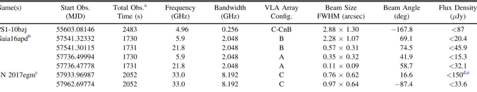
Name(s) Start Obs. Total Obs.a Frequency Bandwidth VLA Array Beam Size Beam Angle Flux Density
(MJD) Time(s) (GHz) (GHz) Config. FWHM(arcsec) (deg) (μJy)
PS1-10bzj 55603.08146 2483 4.96 0.256 C-CnB 2.88×1.30 −167.8 <87 Gaia16apdb 57541.32332 1730 5.9 2.048 B 2.28×1.07 69.1 <20.4 57541.30115 1731 21.8 2.048 B 0.57×0.31 74.5 <45.9 57736.49994 1730 5.9 2.048 A 0.35×0.32 41.9 <15.3 57736.47778 1731 21.8 2.048 A 0.11×0.09 58.7 <32.1 SN 2017egmc 57933.96987 2052 33.0 8.192 C 0.76×0.62 16.6 <150d,e 57962.69774 2052 33.0 8.192 C 0.97×0.64 −87.4 <33.6
Notes.Upper limits are 3σ. a
Including intervening calibrator scans but excluding initial setup scans. b
Alias: SN 2016eay. c
Alias: Gaia17biu. d
This observation was reported in an Astronomer’s Telegram (Coppejans et al.2017).
e
This observation had high noise levels due to poor weather conditions.
Figure 1.Specific radio luminosity at ∼8 GHz (rest frame) for SLSNe-I (red stars) in the context of H-stripped core-collapse explosions(i.e., GRBs (circles) and normal Ic SNe(squares)). Black circles: GRBs at z0.3. Gray circles: GRBs at z>0.3. Gray squares: normal Ic SNe. Blue squares: relativistic Ic SNe. Connected symbols refer to observations of the same object. For display purposes, only the SLSNe-I directly referred to in the text are labeled. Deep radio observations of the closest SLSNe-I, like Gaia16apd and SN 2017egm, clearly rule out on-axis jets of the kind detected in GRBs and probe the parameter space of the weakest engine-driven SNe (like those associated with GRBs 980425 and 100316D). Notably, radio obser-vations of Gaia16apd and SN 2017egm indicate that SLSNe-I can be significantly fainter than normal H-stripped core-collapse SNe as well. References: Immler et al. (2002), Pooley & Lewin (2004), Soria et al. (2004), Soderberg et al. (2005), Perna
et al.(2008), Chandra et al. (2009b,2010), Soderberg et al. (2010b), Corsi et al.
(2011), Chomiuk et al. (2011), Chomiuk et al. (2012a), Chandra & Frail (2012),
Horesh et al.(2013), Margutti et al. (2013b,2013a,2014), Corsi et al. (2014),
Nicholl et al.(2016b), Kasliwal et al. (2016), Palliyaguru et al. (2016), Bright et al.
(2017), Bose et al. (2018), Coppejans et al. (2017), Romero-Canizales et al. (2017).
16Common Astronomy Software Applications package (McMullin et al.
GRB distribution).17At z<0.3, we are consequently sensitive to the entire demographics of long GRBs. For Gaia16apd and SN 2017egm, our limits rule out radio emission of the kind detected from GRBs in the local universe (black points in Figure 1), with the exception of the faint GRB 060218 (for
which there is no evidence for collimation of the fastest ejecta). Notably, for Gaia16apd and SN 2017egm, we can rule out emission of the kind detected from the low-luminosity GRB 980425 associated with SN 1998bw (for which there is also no evidence for collimation of the fastest ejecta). This is of particular relevance, as Nicholl et al. (2016b) found clear
similarities in the nebular spectra of the SLSN 2015bn and the GRB SN 1998bw, which suggests a similar core structure of their stellar progenitors at the time of collapse and possibly also a similar explosion central engine. Radio observations show that this similarity does not extend to the properties of the fastest ejecta of Gaia16apd and SN 2017egm.(We note that for SLSN 2015bn, radio observations were acquired at a much later epoch and do not constrain GRB 980425–like radio emission, as shown in Figure 1; Nicholl et al. 2016a). If the
deepest limits (SN 2017egm and Gaia16apd) are excluded, the rest of the sample still rules out emission of the kind seen in some of the low-luminosity GRBs.
Radio observations of SN 2017egm were acquired at later times than those of the faint GRBs, leaving the possibility of a GRB 060218–like outflow in SLSNe-I still open. To determine the presence of GRB 060218–like emission in SLSNe-I, radio observations at 10 days after the explosion are necessary. This can be seen by considering GRB 060218 in Figure 1: in GRB 060218, the radio luminosity declined by approximately an order of magnitude in thefirst ∼30 days after the explosion, which is the earliest phase for which we have SLSN-I radio observations.
We conclude that this sample of SLSNe-I is not consistent with having on-axis jets of the kind detected in GRBs. The deepest SLSN-I limits also rule out emission from weak, poorly collimated GRBs, with the notable exception of the fast-fading GRB 060218.
4.2. Off-axis Relativistic Jets
4.2.1. Simulation Setup
To constrain the presence of off-axis relativistic outflows in SLSNe-I, we generated a grid of model light curves for off-axis GRB jets using high-resolution, two-dimensional relativistic hydrodynamical jet simulations. For this, we used the broad-band afterglow numerical code Boxfit v2 (van Eerten et al. 2012), which models the off-axis, frequency-dependent
emission as the jet slows and the radiation becomes less beamed. We then compared the collective ∼8 GHz (central frequencies in the range 6.1–10.6 GHz, as indicated in Table1)
radio upper limits in our sample to each light curve to determine if the observations rule out that particular set of parameters. These frequencies provide the most stringent constraints on the jet parameters, as they include the deepest limits, were taken at the earliest and latest times, and have the densest time coverage. To do this, we made the necessary assumption that every SLSN-I in our sample is powered by the same mechanism(and jet/environment properties), i.e., a given
set of parameters is ruled out if they are ruled out for at least one SLSN-I. The radio light curves are not sufficiently well-sampled to do this analysis individually. An illustration of this process is given in Figure2.
The modeled radio light curves depend on the following input parameters: (1) the isotropic equivalent kinetic energy Ek,iso of the outflow; (2) the density of the medium, where
either an interstellar medium (ISM)-like medium (nCSM
constant) or a wind-like medium (rCSM= ˙ (M 4pR v2 w))
produced by a constant progenitor mass-loss rate M˙ can be chosen; (3) the microphysical shock parameters B and òe, which are the postshock energy fraction in the magneticfield and electrons, respectively (see Sironi et al. 2015 for more details); (4) the jet opening angle θj; and(5) the observer angle with respect to the jet axis θobs (hereafter referred to as the observer angle). We fixed the power-law index of the shocked electron energy distribution to p=2.5, as it typically varies in the range 2–3 from GRB afterglow modeling (e.g., Curran et al.2010and Wang et al.2015). Unless otherwise specified,
we will report mass-loss rates M˙ for an assumed wind velocity of vw=1000 km s-1, which is representative of compact massive stars like Wolf–Rayet stars.
We explore two physical scenarios for the interstellar
medium, namely, ISM-like (10 3cm 3 n 10 cm
CSM 2 3
- - - )
and wind-like (10-8M yr-1M 10-3M yr-1
˙ ), for two
jet collimation angles(q = and 30°), three observer anglesj 5 (qobs=30, 60°, and 90°) and isotropic kinetic energies in the range 1050ergEk,iso1055erg. These values are represen-tative of the parameters that are derived from accurate modeling of the broadband afterglows of GRBs(e.g., Schulze Figure 2.Example illustrating how the collective SLSN-I∼8GHz limits and the model jet light curves are used to test a set of parameters. Two models for off-axis jets are shown for an ISM profile CSM (constant density,rCSM), with
30 j
q = , Ek,iso=1053erg, nCSM=10cm−3,e=0.1, andB=0.01. The red squares and black dots show the emission for the jet positioned at angles of
90 obs
q = andqobs=45, respectively. The radio limits rule out this set of parameters for both models, as they are lower than the predicted specific luminosities for either angle. The radio emission from a jet at a larger off-axis angle will peak later than it would at smaller angles, as the radiation is initially beamed away from the observer and will take longer to spread into the line of sight. Late-time observations are consequently necessary to constrain off-axis jets. For this set of parameters, the latest two observations(at 203 and 318 days for Gaia16apd and SN 2015bn, respectively) are more constraining for the
90 obs
q = jet than the deepest radio limits, as the emission peaks later on.
17
Since the VLA upgrade, more sensitive observations of GRBs at z<0.3 have consistently yielded detections(Zauderer et al.2012; van der Horst2013; Horesh et al.2015; Kamble2015; Laskar et al.2016).
et al. 2011; Laskar et al. 2013; Perley et al. 2014; Laskar et al.2016).
In Figures3and4, we present the results from the entire set of simulations for the range of òe and òB typically used in the literature. Relativistic shock simulations showòe=0.1 (e.g., Sironi et al.2015), and òBis less constrained thanòe. The distribution for òBderived from GRB afterglow modeling is centered on 0.01 and typically spans 10−4to 0.1, with a few claims for smaller values down to≈10−7(e.g., Santana et al.2014). In the text, we discuss
the results for thefiducial parameterse=0.1andB=0.01but show the results for other typical values of the microphysical shock parameters in thefigures.
At radio frequencies, the afterglow radiation (i.e., radiation arising from the jet interaction with the medium) consists of synchrotron emission. Both synchrotron emission and synchro-tron self-absorption (SSA) are accounted for in the afterglow models. Free–free absorption is not significant for the circumstellar medium (CSM) densities and blast-wave velo-cities that we consider here. Following Weiler et al.(1986), and
considering a wind medium with the highest mass-loss rates investigated here(i.e., M =10-3M yr-1
˙ ), we find the free–
free optical depth t <ff 0.04 for frequencies greater than 5 GHz at time t>26 days. The SLSN-I 2017egm was observed at 1.6 GHz at∼39 days since explosion (Table1). In
this case, we estimate a<15% flux reduction due to free–free absorption for the largest densities considered in this study, with no impact on our major conclusions. For the ISM-like densities considered below, free–free absorption is always negligible.
We consider the radio limits from the entire sample of SLSNe-I in this analysis. Note that the constraints that we derive are not driven solely by one SLSN-I. Although the limits for SN 2017egm are significantly deeper than for the rest of the sample, we only have early-time coverage for this system. As late-time observations are more constraining for off-axis jets, the other systems in our sample still provide meaningful constraints for off-axis jets (see Figure 2). SN
2017egm exploded in 2017 June, so our limits only extend to Figure 3.Constraints on jetted outflows in the sample of radio-observed SLSNe-I, assuming the progenitor produced a wind density profile (r µr-2) in the surrounding medium. The symbol colors represent jet opening angles ofq = (black) andj 5 q =j 30 (gray). Symbol sizes indicate the observer angle (q ) for whichobs we can rule out the corresponding jet, with larger symbols corresponding to largerq . Red crosses indicate that the parameters could not be ruled out. The topobs (bottom) panels aree=0.1(òe=0.01), and the left (right) panels are òB=0.0001 (òB=0.01). Note: In the top left panel, highly collimated jets (q = ) withj 5 Ek,iso1053erg and progenitor mass-loss rates of M˙ 10-4Myr-1are ruled out for all observer angles. The“outlier” at Ek,iso=1055erg was a sampling effect, where the upper limit was negligibly more luminous than the model atqobs=90.
47 days (considering only the ∼8 GHz observations). Radio observations of this object at later times will place the strongest constraints on off-axis jets in SLSNe-I to date. We will consequently continue radio monitoring of SN 2017egm.
4.2.2. Results: Ek,iso and M˙ Phase Space
Figures 3 and4 show the constraints that the upper limits on the radio luminosity of the sample of SLSNe-I place on off-axis jets expanding into a wind profile medium and an ISM profile medium, respectively. First, consider a wind profile medium and jets that are off-axis and highly collimated (q = , like those detected in GRBs). Forj 5 e=0.1 and
0.01 B
= (top right panel), these off-axis GRB-like jets are ruled out regardless of the observer angle for M ˙
M
10-4 yr-1
and Ek,iso1053erg (this is within the energy
range of the observed GRB population). Mass-loss rates such as these are typically found in the winds of extreme red supergiants (e.g., Smith et al. 2009; Smith 2014) and
luminous blue variables (Groh 2014; Smith 2014). To put
this in context, Figure 5 shows the mass-loss rates and equivalent densities at 1016cm (assuming a 1000 km s−1
progenitor wind speed) for other H-poor stellar explosions. Specifically, mass-loss rates of this order (M 10-4M yr-1
˙ )
have been inferred for some SNe Ibc(Figure5and references therein), as well as for SNe IIb18 with yellow supergiant progenitors (e.g., SN 2013df19; Kamble et al. 2016). The
precluded
phase space for highly collimated, off-axis jets with M ˙
M
10-4 yr-1
and Ek,iso1053is indicated in Figure5.
GRB-like jets are not ruled out for the lower-density environments inferred for some GRBs.
If instead we consider off-axis jets that are less collimated (q =j 30) than cosmological GRBs, we can probe to deeper limits, as the jet is less collimated to start with and more kinetic energy is coupled to it (with respect to a more collimated jet with the same Ek,iso). In this case, regardless of the observing
angle, we can rule out scenarios where M 10-5M yr-1
˙ and
Ek,iso1053erg (Ek <1050erg), as shown in Figure 3 (for
Figure 4.Constraints on jetted outflows in the sample of radio-observed SLSNe-I for a constant density profile in the surrounding medium. See the caption of Figure3
for a full description of the symbols. Note: In the top right panel, highly collimated jets(q = ) with Ej 5 k,iso1051erg in environments with nCSM=10cm−3are ruled out for all observer angles.
18
Type IIb SNe are a class that originally shows H lines but transitions to Type Ib–like (no H lines) over time.
19
Note that we assume a 1000 km s−1wind here and have adjusted the mass-loss rate in Kamble et al.(2016) accordingly.
òe=0.1 and òB=0.01). This parameter space is illustrated in Figure 5. A significant fraction of the galactic Wolf–Rayet population (Vink & de Koter 2005; Crowther 2007) and
luminous blue variables (e.g., Vink & de Koter 2002; Smith et al.2004), as well as the most luminous O-type stars (e.g., de
Jager et al.1988; van Loon et al.2005), show mass-loss rates in
this range. Off-axis jets of this kind with Ek,iso1053erg would also be precluded in the most dense environments inferred for GRBs and for most of the observed population of hydrogen-stripped SNe (assuming a 1000 km s−1wind).
In Section 4.1, we discussed how this sample of SLSNe-I ruled out on-axis jets of the kind seen in low-luminosity (less-collimated) GRBs, with the exception of GRB 060218. Now consider less-collimated jets (q =j 30) that are aligned only slightly off-axis—within 30° of our line of sight. Jets of this
kind are ruled out down to clean environments of
M 10-8M yr-1
˙ , where Ek,iso1051erg (Figure 3, for
òe=0.1 and òB=0.01). Assuming a progenitor wind speed of 1000 km s−1, this parameter space precludes the environments of all of the detected SNe Ibc and most of the GRBs detected to date(see Figure5).
For comparison, Figure4gives the equivalent constraints for a constant density environment (modeling of GRB afterglows sometimes indicates a better fit to ISM environments; e.g., Laskar et al. 2014). For e=0.1 and òB=0.01 (top right panel), a collimated jet withq = is ruled out regardless ofj 5 the observer angle for nCSM10 cm-3 and Ek,iso1051erg.
A jet with q =j 30 is ruled out for nCSM1 cm-3 and Ek,iso1051erg. Deeper constraints are obtained for jets with their axes aligned within 30° or 60° of our line of sight. Specifically, the jets withq = and observer angles of 30°j 5 are excluded down to nCSM10-3cm-3.
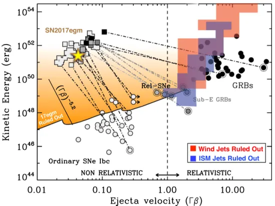
4.2.3. Results: Ek and Gb Phase Space
Engine-driven explosions (i.e., GRBs, subenergetic GRBs, and relativistic SNe) are clearly distinguished from normal spherical core-collapse SNe by aflatter kinetic energy profile of their ejecta(e.g., Soderberg et al.2006a). For an engine-driven
explosion, a larger fraction of the kinetic energy is contained in the fast-moving ejecta than in the slow-moving ejecta, in contrast to a hydrodynamical explosion. This is illustrated in Figure6, where we plot the kinetic energy in the slow- and fast-moving ejecta(joined by a dashed line to guide the eye) for the H-poor explosions where these properties have been measured. For a pure hydrodynamical explosion, we would expect a profile of Ek~ G( b)-5.2, while GRBs have significantly flatter
profiles (Tan et al.2001). A flat energy profile for the SLSNe-I
would suggest an engine-driven explosion.
We have excluded a region of the Ek-versus- bG phase space
in Figure6for this sample of SLSNe-I based on the limits from our simulations. Specifically, for a collimated (q =j 30) jet (ruled out at all observer angles), we deduce limits based on the excluded combinations of mass-loss rate and isotropic kinetic energy (Figures 3 and 4) as follows. Applying the standard
formulation of thefireball dynamics with expansion in a wind-like and ISM-wind-like environment(e.g., Chevalier & Li2000), the
bulk Lorentz factor of the downstreamfluid behind the shock front is
E A t
18.7 k,iso 1054erg1 4 * 0.1 1 4 1 day 1 4
G ~ ( ) ( )- ( )
-for a wind profile medium and
E n t
10.1 k,iso 1054erg1 8 CSM 0.1cm 3 1 8 1 day 3 8
G ~ ( ) ( - -) ( )
-for an ISM profile medium. Here G =s 2G is the shock Lorentz factor, A* is the wind parameter characterizing Figure 5.Density in the SN immediate surroundings as a function of the explosion’s fastest ejecta for H-stripped core-collapse SNe (gray circles) and GRBs (black circles). The red and blue shaded areas mark the regions of the parameter space that are ruled out for any observer angle by our simulations of relativistic jets (both
30 j
q = andq = are included) in wind and ISM environments, respectively (forj 5 e=0.1andòB=0.01). The orange shaded area marks the region ruled out by the
radio limits on SN 2017egm for an uncollimated outflow. The mass-loss scale on the right y-axis is for vw=1000 km s-1. The velocity of the fast-moving ejecta has been computed at t=1 days (rest frame). The horizontal dashed lines indicate the mass-loss rates measured in the Galaxy for Wolf–Rayet stars (Crowther2007) and
WN3/O3 stars (Massey et al.2015). References: Berger et al. (2003a,2003b), Frail et al. (2006), Soderberg et al. (2006a), Chandra et al. (2008), Soderberg et al.
(2008), Cenko et al. (2010), Soderberg et al. (2010b,2010a), Cenko et al. (2011), Troja et al. (2012), Cano (2013), Horesh et al. (2013), Laskar et al. (2013), Margutti
the density of the wind-generated CSM, and A* =1 for
M˙ =10-5M yr-1
☉ and vw=1000 km s-1. In Figure 6, we
plot the beaming-corrected kinetic energy Ek=Ek,iso
1-cosqj
( ) and estimate the specific momentum of the fastest ejecta at an arbitrary time of 1 day post-explosion(rest frame). The excluded phase spaces for a jet collimated toqj30 are shaded in red and blue in Figure6for a wind and ISM medium, respectively.
The excluded phase space does not constrain the slope of the kinetic energy profile to the extent where we can confirm or rule out the presence of a central engine in this sample of SLSNe-I. Based on our simulations, we ruled out off-axis collimated (q =j 30) jets at M˙ 10-5Myr-1 and Ek,iso
1052erg for every observing angle. GRB-like jets exploding in
less-dense environments than we rule out will have faster-moving ejecta and thus appear to the right of the excluded phase space in this figure. This phase space associated with faster-moving ejecta is not ruled out because these jets are associated with large Ek,iso and very low densities. As the
radio emission is produced in the shock front between the jet and the CSM, at low densities, the radio luminosity will be lower and more difficult to rule out, especially if it is off-axis.
5. Constraints on Uncollimated Outflows
Despite the fact that SLSNe-I are significantly more luminous (∼10–100 times) than “normal” Type Ic SNe at optical wavelengths, the deepest SLSN-I limits indicate that they can be significantly fainter than even some normal SNe Ic at radio wavelengths(see Figure1). Here we analyze our radio
limits in the context of uncollimated(spherical) outflows. Among H-stripped core-collapse SNe without collimated outflows, relativistic SNe qualify as a separate class. Relati-vistic SNe are characterized by mildly relatiRelati-vistic ejecta, bright radio emission—but faint X-ray emission that clearly sets relativistic SNe apart from subenergetic GRBs—and a kinetic energy profile Ek(Gb) (Figure 6) that is suggestive of the
presence of a central engine driving the explosion(Bietenholz et al.2010; Soderberg et al.2010b; Chakraborti & Ray 2011; Margutti et al.2014; Chakraborti et al.2015). These observed
properties are attributed to a scenario where a jet is present but fails to successfully break through the stellar envelope, possibly due to a shorter-lived engine or a larger envelope mass(Lazzati et al.2012; Margutti et al.2014; see also Mazzali et al.2008).
To date, only two relativistic SNe, 2009bb and 2012ap, and one candidate(iPTF17cw; Corsi et al.2017) are known. As there is
Figure 6.Kinetic energy profile of the ejecta of H-poor cosmic explosions, including ordinary Type Ibc SNe, relativistic SNe, GRBs, and subenergetic GRBs. The symbol colors indicate the class of object, namely, black for GRBs, gray for relativistic SNe, and white for ordinary SNe Ibc. Shaded areas mark the constraints on the properties of the SLSN-I fastest ejecta. Squares and circles are used for the slow-moving and fast-moving ejecta, respectively, as measured from optical(slow ejecta) and radio(fast ejecta) observations. An additional circle surrounding a point indicates that the object showed a broad-line optical spectrum. The velocity of the fast-moving ejecta has been computed at t=1 days (rest frame). The ejecta kinetic energy profile of a pure hydrodynamical explosion is also marked as a reference (Ek~ G( b)-5.2; Tan et al.2001). The blue and red areas identify the regions of the parameter space of the fast-moving ejecta that are ruled out based on our simulations of relativistic jets expanding in an ISM and wind-like environments, respectively(fore=0.1andòB=0.01). Only jet models that are ruled out for any
observer angle are shown here. The orange shaded area identifies the region of the parameter space that is ruled out based on our simulations of radio emission from noncollimated outflows and the radio limits on SN 2017egm. The location of the slowly moving ejecta of SN 2017egm is shown with a star. References: Berger et al. (2003a,2003b), Frail et al. (2006), Soderberg et al. (2006a), Chandra et al. (2008), Soderberg et al. (2008), Cenko et al. (2010), Soderberg et al. (2010b,2010a),
Cenko et al.(2011), Ben-Ami et al. (2012), Sanders et al. (2012), Troja et al. (2012), Cano (2013), Horesh et al. (2013), Laskar et al. (2013), Margutti et al. (2013a),
Mazzali et al.(2013), Milisavljevic et al. (2013), Xu et al. (2013), Corsi et al. (2014), Guidorzi et al. (2014), Kamble et al. (2014), Margutti et al. (2014), Perley et al.
no evidence for the beaming of the radio emission from relativistic SNe(Bietenholz et al.2010; Soderberg et al.2010a; Chakraborti et al.2015), the radio limits on SLSNe-I 2017egm,
Gaia16apd, and, to a lesser extent, 2012il clearly rule out the radio luminosities associated with relativistic SNe (Figure 1).
These observations indicate some key difference of the blast-wave and environment properties of SLSNe-I and relativistic SNe that we quantify below with simulations of the radio emission from uncollimated ejecta.
The SN shock interaction with the medium, previously sculpted by the stellar progenitor mass loss, is a well-known source of radio emission in young SNe(e.g., Chevalier1982; Weiler et al.1986; Chevalier & Fransson2006). The SN shock
wave accelerates CSM electrons into a power-law distribution
N( )g µg-p above a minimum Lorentz factor m
g . Radio
nonthermal synchrotron emission originates as the relativistic electrons gyrate in amplified magnetic fields. The result is a bell-shaped radio spectrum peaking at frequency n andp cascading down to a lower frequency as the medium becomes optically thin to SSA. In the case of H-stripped core-collapse SNe, p ~ is usually inferred, and SSA dominates over free3 – free absorption (e.g., Chevalier & Fransson 2006). The
self-absorbed radio spectrum scales as F µn5 2
n below n andp
F µn p 1 2
n - -( ) aboven (Rybicki & Lightmanp 1979). We generated a grid of radio spectral models with p=3,np between 0.1 and 60 GHz, and peak spectral luminosity Lnpin the range 5´1026–1029erg s-1Hz-1. The comparison to the
SLSN-I radio limits (at all frequencies) leads to robust constraints on the time-averaged velocity of the shock wave ( bG in Figure 1), total energy required to power the radio
emission (E), amplified magnetic field (B), and progenitor mass-loss rate (M˙). Our calculations assume a wind-like medium with fiducial microphysical parameterse=0.1and
0.01 B
= . Following Chevalier(1998), Chevalier & Fransson
(2006), and Soderberg et al. (2012), for SSA-dominated SNe,
the shock-wave radius is given by
R L B L E B R M L t M 3.3 10 10 erg s Hz 5 GHz cm, 0.70 10 erg s Hz 5 GHz G, 12 , 0.39 10 0.1 10 erg s Hz 5 GHz 10 days yr . e B p e B p B B e B p p 15 1 19 26 1 1 9 19 1 4 19 26 1 1 2 19 2 3 5 1 8 19 26 1 1 4 19 2 2 1 p p p n n n » ´ ´ » ´ = » ´ ´ ´ ´ n n n - - -- - -- - -- -( ) ( ) ( ) ( ) ( ) ( ) ˙ ( ) ( ) ( ) ( ) ( ) ☉
Based on these simulations, we find that the radio limits on the SLSN-I 2017egm produce interesting constraints in the M˙ ,
Ek, andG phase space (orange shaded area in Figuresb 5and
6). At any given velocity of the fastest ejecta, the limits on SN
2017egm rule out Ek>1048erg coupled to the fastest ejecta (Figure 6) and the densest environments found in association
with H-stripped core-collapse SNe (Figure 5). Current limits,
however, do not constrain the slope of the Ek(Gb) profile or
rule out the region of the parameter space populated by spherical hydrodynamical collapses with Ek<1048erg in their fastest ejecta(Figure 6).
6. Summary and Conclusions
We have compiled all of the radio observations of SLSNe-I published to date and presented three new observations (a sample of nine SLSNe-I). Based on these limits, we constrain the subparsec environments and fastest ejecta in this sample of SLSNe-I for the case that a relativistic jet or an uncollimated outflow is present. For this analysis, we make the necessary assumption that the jet/environment properties do not vary within this sample of SLSNe-I. These are our main results.
1. In this sample of SLSNe-I, we rule out collimated on-axis jets of the kind detected in GRBs.
2. We do not rule out the entire parameter space for off-axis jets in this sample, but we do constrain the energies and circumstellar environment densities if off-axis jets are present.
3. If the SLSNe-I in this sample have off-axis GRB-like (collimated toq = ) jets, then the local environment isj 5 of similar(or lower) density as that of the detected GRBs. Specifically, if off-axis jets of this kind are present, then they have energies Ek,iso<1053erg(Ek<4 ´1050erg)
in environments shaped by progenitors with mass-loss rates M <10-4M yr-1
˙ (for microphysical shock
para-meterse=0.1andB=0.01). This would, for example, exclude jets with Ek>4 ´1050erg if the progenitor mass-loss rates were of the order typically found in the winds of extreme red supergiants and luminous blue variables(and inferred for some SNe Ibc and IIb). 4. If this sample of SLSNe-I produced off-axis jets that are
less collimated (q =j 30) than cosmological GRBs, then the jets must have energies Ek,iso<1053erg (Ek<1050erg) and occur in environments shaped by progenitors with mass-loss rates M <10-5M yr-1
˙ .
This precludes jets of this kind with Ek<1050erg for the mass-loss rates inferred for most of the observed population of hydrogen-stripped SNe and the most dense environments inferred for GRBs.
5. The deepest SLSN-I limits rule out emission from faint uncollimated GRBs (“subluminous” or “subenergetic” GRBs), including GRB 980425 but with the exception of GRB 060218. To successfully probe emission at the level of all poorly collimated GRBs(like GRB 060218), radio observations of SLSNe-I in the local universe(z0.1) need to be taken10 days after explosion.
6. The radio limits of this sample of SLSNe-I rule out radio luminosities associated with relativistic SNe and thus likely indicate some key difference of the blast-wave and environment properties between these two classes of objects. Significant differences in the respective struc-tures of the progenitor stars and/or jet longevity may also affect the ability of the central engine’s jet to successfully break through the stellar envelope.
7. We only partially rule out the phase space associated with uncollimated outflows, such as the kind seen in ordinary Type Ibc SNe.
8. For SN 2017egm(the closest SLSN-I observed at radio wavelengths to date), we can constrain the energy of a possible uncollimated outflow to Ek 1048erg, which is consistent with the kinetic energy associated with the fastest-moving material in ordinary Type Ibc SNe.
Radio observations of SLSNe-I are a powerful tool to constrain the central engine properties and subparsec environ-ments of these luminous, H-stripped stellar explosions. To fully constrain the outflow and environment properties, a combina-tion of both early-time and late-time coverage is needed. Specifically, to probe emission at the level of all poorly collimated GRBs (like GRB 060218), radio observations of SLSNe-I in the local universe (z0.1) need to be taken 10 days after explosion. Late-time radio observations taken hundreds of days post-explosion are necessary to detect off-axis collimated jets in these systems. We will be able to constrain this much more efficiently with more sensitive radio telescopes that are coming online or planned, such as
MeerKAT, the next-generation VLA (ngVLA; McKinnon
et al. 2016), and the Square Kilometre Array (SKA; Carilli &
Rawlings2004).
This research made use of the Open Supernova Catalog (Guillochon et al. 2017) and NASA’s Astrophysics Data
System Bibliographic Services. The National Radio Astronomy Observatory is a facility of the National Science Foundation operated under cooperative agreement by Associated Univer-sities, Inc. CG acknowledges the University of Ferrara for use of the local HPC facility cofunded by the “Large-Scale Facilities 2010” project (grant 7746/2011). We thank the University of Ferrara and INFN-Ferrara for the access to the COKA GPU cluster. Development of the BOXFIT code was supported in part by NASA through grant NNX10AF62G issued through the Astrophysics Theory Program and by the NSF through grant AST-1009863. Simulations for BOXFIT version 2 have been carried out in part on the computing facilities of the Computational Center for Particle and Astrophysics(C2PAP) of the research cooperation “Excellence
Cluster Universe” in Garching, Germany. DC and RM
acknowledge partial support from program Nos.
NNX16AT51G and NNX16AT81G provided by NASA through the Swift Guest Investigator Programs. Support for BAZ is based in part while serving at the NSF. At the time of the observations, LC was a Jansky Fellow of the National Radio Astronomy Observatory. GM acknowledges funding support from the UnivEarthS Labex program of Sorbonne Paris Cité (ANR-10-LABX-0023 and ANR-11-IDEX-0005-02) and from the French Research National Agency, CHAOS project ANR-12-BS05-0009.
Appendix
Brief Description of the SLSNe-I in Our Sample A.1. PTF09cnd
PTF09cnd was detected by the Palomar Transient Factory during commissioning and was one of the systems that originally defined the SLSN class (Quimby et al. 2011).
Properties of the host galaxy are given in Neill et al.(2011) and
Perley et al. (2016). X-ray observations at 0.3–10 keV
produced nondetections with unabsorbed fluxes in the range 10-15–10-13erg s−1cm−2 (Levan et al. 2013; Margutti et al.
2017a). Radio observations of PTF09cnd are reported on in
Chandra et al. (2009b,2010) (see Table1).
A.2. PS1-10awh
PS1-10awh was discovered in 2010 October in the Pan-STARRS1 Medium Deep Survey while on the rise to peak
(Chomiuk et al.2011). UV/optical photometry and time-series
spectroscopy from day −21 to 26 is presented in Chomiuk et al.(2011). Lunnan et al. (2014) detected the host galaxy at
MF606W =27mag with the Hubble Space Telescope. Chomiuk et al. (2011) observed PS1-10awh at radio wavelengths (see
Table1).
A.3. PS1-10bzj
PS1-10bzj was discovered in the Pan-STARRS (Chambers et al.2016) Medium Deep Survey and classified as a SLSN-I
with a peak magnitude of around −21.4 mag (Lunnan et al.
2013). Lunnan et al. found that the luminosity cannot be
powered solely by radioactive nickel decay, but a magnetar or interaction model can explain the observed properties(although intermediate-width spectral lines are predicted by the interac-tion model, none were detected). Radio observations of this SN are presented here for thefirst time (see Table2).
A.4. PS1-10ky
PS1-10ky was discovered near peak brightness in the
Pan-STARRS1 Medium Deep Survey at z=0.9558 (Chomiuk
et al.2011). At peak, its bolometric magnitude was −22.5 mag
(see Chomiuk et al.2011). No host has been detected for this
SN (Chomiuk et al. 2011; Lunnan et al. 2015; McCrum et al. 2015). Radio observations of PS1-10ky have been
presented in Chomiuk et al.(2011); see Table1. A.5. SN 2012il
SN 2012il (alternatively PS1-12fo or CSS120121:094613 +195028) was independently discovered in the Pan-STARRS1 3Pi Faint Galaxy Supernova Survey(Smartt et al.2012) and the
Catalina Real-time Transient Survey (Drake et al. 2012) on
2012 January 19 and 21, respectively. Smartt et al. (2012)
classified it as an SLSN-I at z=0.175. Based on the late-time luminosity decline rate and the short diffusion times at peak, Inserra et al.(2013) favored the magnetar model. See Lunnan
et al.(2014) for optical spectroscopy of the host galaxy. X-ray
observations of SN 2012il in the 0.2–10 keV band yielded nondetections with upper limits on the unabsorbedflux in the range 10-13–10-12erg cm−2s−1 (Levan et al. 2013; Margutti
et al.2017b). The radio observations of this system were taken
by Chomiuk et al.(2012b); see Table 1. A.6. SN 2015bn
SN 2015bn (alternatively PS15ae, CSS141223:113342 +004332, or MLS150211:113342+004333) was discovered by the Catalina Real-time Transient Survey(Drake et al.2009)
and the Pan-STARRS Survey for Transients (Huber
et al. 2015). It was classified as an SLSN-I by Le Guillou
et al.(2015), which was confirmed by Drake et al. (2015). In
UV(obtained with Swift) to NIR observations from −50 to 250 days from optical peak, Nicholl et al.(2016a) found that it was
slowly evolving and showed large undulations (on timescales of 30–50 days) superimposed on this evolution in the light curve. The nature of these undulations is discussed in Nicholl et al.(2016a) and Yu & Li (2017).
Nebular phase observations of SN 2015bn (Nicholl et al.
2016b; Jerkstrand et al.2017) indicate that it is powered by a
central engine(Nicholl et al.2016b). From spectropolarimetric
axisymmetric geometry and found that the evolution could be consistent with a central engine. Additional polarimetric observations can be found in Leloudas et al. (2017). X-ray
observations at 0.3–10 keV produced nondetections with unabsorbed fluxes that were predominantly in the range 10-14–10-13erg s−1cm−2 (Nicholl et al. 2016a; Inserra et al.
2017; Margutti et al.2017a). Radio observations of SN 2015bn
are presented in Nicholl et al. (2016a) (see Table1).
A.7. iPTF15cyk
The SLSN-I iPTF15cyk was detected on 2015 September 17 in optical follow-up observations of the gravitational-wave source GW150914 by the intermediate Palomar Transient Factory (Kasliwal et al. 2016). Further spectroscopic and
multiwavelength observations confirmed it as an SLSN-I (Kasliwal et al. 2016). X-ray observations (Kasliwal
et al. 2016) gave an upper limit on the unabsorbed flux of
1.3´10-13erg cm−2s−1. Radio observations (Palliyaguru
et al. 2016and Kasliwal et al.2016; see Table1) were taken
as part of the first broadband campaign to search for an electromagnetic counterpart to an Advanced Laser Interferom-eter Gravitational-Wave Observatory (LIGO) gravitational-wave trigger (Abbott et al.2016).
A.8. Gaia16apd
Gaia16apd(alternatively SN 2016eay) was discovered by the Gaia Photometric Survey(Gaia Collaboration et al.2016) and
classified as an SLSN-I by Kangas et al. (2016). At early times,
it was extremely bright at UV wavelengths (peaking at −23.3 mag) in comparison to other SN classes (Blagorodnova et al. 2016; Kangas et al. 2017; Yan et al. 2017b). Based on
later-time UV (observations obtained with Swift) and optical observations, Nicholl et al. (2017b) concluded that this is due
to a more powerful central engine rather than interaction with the surrounding medium or a lack of UV absorption. Nicholl et al. found that the bestfit for a magnetar central engine has a spin period of 2 ms and magnetic field of 4×10¹⁴ G (in agreement with Kangas et al. 2017). Radio observations of
Gaia16apd are presented here for the first time (see Table2).
A.9. SN 2017egm
SN 2017egm (alternatively Gaia17biu) was discovered by the Gaia satellite on 2017 May 26 and was originally classified as a Type II SN (Xiang et al.2017). Dong et al. (2017) then
reclassified it as an SLSN-I at z=0.030721, making it the closest SLSN-I discovered to date.
Although an initial X-ray detection of the SN was claimed (Grupe et al.2017a), it was later found that the X-ray emission
was more likely associated with star formation in the host galaxy, NGC 3191 (Bose et al. 2018; Grupe et al. 2017b).
Several radio observations were taken at different frequencies (see Table 1 for details), but SN 2017egm was not detected (Bose et al. 2018; Bright et al. 2017; Coppejans et al. 2017; Romero-Canizales et al.2017).
The host galaxy, NGC 3191, is unlike those of other SLSNe-I. It is a metal-rich( 1.3Z» at the radial offset of the SN) massive
spiral galaxy with a high star formation rate of»15M yr-1
and
mass of »1010.7M
(Nicholl et al. 2017a; see also Bose
et al.2018). Izzo et al. (2018), however, showed that there are
spatial variations in the host properties, and the local
environment of SN 2017egm is not so unusual. NGC 3191 is also a known radio source: it was detected at 1.4 GHz in the Faint Images of the Radio Sky at Twenty Centimeters(FIRST) survey with a peakflux density of 1.63±0.13 mJy beam−1and an integrated flux density of 15.96±0.13 mJy (White et al. 1997). Furthermore, NGC 3191 was detected at
1.8±0.1 mJy at 15.5 GHz (Bright et al. 2017) and detected
and resolved at 10 GHz (Bose et al. 2018). In our 33 GHz
observations, we do not detect the host galaxy to a 3σ upper limit of 150μJy beam−1. ORCID iDs D. L. Coppejans https://orcid.org/0000-0001-5126-6237 R. Margutti https://orcid.org/0000-0003-4768-7586 C. Guidorzi https://orcid.org/0000-0001-6869-0835 L. Chomiuk https://orcid.org/0000-0002-8400-3705 K. D. Alexander https://orcid.org/0000-0002-8297-2473 E. Berger https://orcid.org/0000-0002-9392-9681 M. F. Bietenholz https://orcid.org/0000-0002-0592-4152 W. Fong https://orcid.org/0000-0002-7374-935X A. MacFadyen https://orcid.org/0000-0002-0106-9013 G. Migliori https://orcid.org/0000-0003-0216-8053 D. Milisavljevic https://orcid.org/0000-0002-0763-3885 M. Nicholl https://orcid.org/0000-0002-2555-3192 J. T. Parrent https://orcid.org/0000-0002-5103-7706 References
Abbott, B. P., Abbott, R., Abbott, T. D., et al. 2016,ApJL,826, L13
Angus, C. R., Levan, A. J., Perley, D. A., et al. 2016,MNRAS,458, 84
Barkat, Z., Rakavy, G., & Sack, N. 1967,PhRvL,18, 379
Ben-Ami, S., Gal-Yam, A., Filippenko, A. V., et al. 2012,ApJL,760, L33
Berger, E., Kulkarni, S. R., Frail, D. A., & Soderberg, A. M. 2003a,ApJ,
599, 408
Berger, E., Kulkarni, S. R., Pooley, G., et al. 2003b,Natur,426, 154
Bietenholz, M. F., Soderberg, A. M., Bartel, N., et al. 2010,ApJ,725, 4
Blagorodnova, N., Yan, L., Quimby, R., et al. 2016, ATel,9074
Bose, S., Dong, S., Pastorello, A., et al. 2018,ApJ,853, 57
Bright, J., Mooley, K., Fender, R., et al. 2017, ATel, 10538 Cano, Z. 2013,MNRAS,434, 1098
Carilli, C. L., & Rawlings, S. 2004,NewAR,48, 979
Cenko, S. B., Frail, D. A., Harrison, F. A., et al. 2010,ApJ,711, 641
Cenko, S. B., Frail, D. A., Harrison, F. A., et al. 2011,ApJ,732, 29
Chakraborti, S., & Ray, A. 2011,ApJ,729, 57
Chakraborti, S., Soderberg, A., Chomiuk, L., et al. 2015,ApJ,805, 187
Chambers, K. C., Magnier, E. A., Metcalfe, N., et al. 2016, arXiv:1612.05560
Chandra, P., Cenko, S. B., Frail, D. A., et al. 2008,ApJ,683, 924
Chandra, P., Dwarkadas, V. V., Ray, A., Immler, S., & Pooley, D. 2009a,ApJ,
699, 388
Chandra, P., & Frail, D. A. 2012,ApJ,746, 156
Chandra, P., Ofek, E. O., Frail, D. A., et al. 2009b, ATel,2241
Chandra, P., Ofek, E. O., Frail, D. A., et al. 2010, ATel,2367
Chatzopoulos, E., & Wheeler, J. C. 2012,ApJ,760, 154
Chatzopoulos, E., Wheeler, J. C., Vinko, J., et al. 2011,ApJ,729, 143
Chatzopoulos, E., Wheeler, J. C., Vinko, J., Horvath, Z. L., & Nagy, A. 2013,
ApJ,773, 76
Chen, T.-W., Nicholl, M., Smartt, S. J., et al. 2017c,A&A,602, A9
Chen, T.-W., Schady, P., Xiao, L., et al. 2017b,ApJL,849, L4
Chen, T.-W., Smartt, S. J., Jerkstrand, A., et al. 2015,MNRAS,452, 1567
Chen, T.-W., Smartt, S. J., Yates, R. M., et al. 2017a,MNRAS,470, 3566
Chevalier, R. A. 1982,ApJ,258, 790
Chevalier, R. A. 1998,ApJ,499, 810
Chevalier, R. A., & Fransson, C. 2006,ApJ,651, 381
Chevalier, R. A., & Irwin, C. M. 2011,ApJL,729, L6
Chevalier, R. A., & Li, Z.-Y. 2000,ApJ,536, 195
Chomiuk, L., Chornock, R., Soderberg, A. M., et al. 2011,ApJ,743, 114
Chomiuk, L., Soderberg, A., Margutti, R., et al. 2012a, ATel,3931
Chomiuk, L., Soderberg, A. M., Moe, M., et al. 2012b,ApJ,750, 164