Facolt`
a di Scienze Statistiche
Corso di Laurea Specialistica in Scienze Statistiche,
Demografiche e Sociali
Tesi di Laurea
Innovative statistical methods
for the construction
of composite scales
from ordinal variables
with application to business
and management data
September 15, 2009
Relatore: Ch.mo Prof. Fortunato Pesarin Correlatore: Ch.mo Prof. Luigi Salmaso
Laureando: Enrico Tonini - 600413
Preface 1
1 Analysis of Likert’s scales 3
1.1 Introduction: a brief summary of types of variables . . . 3 1.2 Likert’s scales: the peculiarities of this type of data . . . 5 1.2.1 Features and construction of a Likert’s scale . . . 5 1.2.2 The literary “disputation” between methodologic
statis-ticians and more pragmatic economists . . . 5 1.3 A first more traditional and pragmatic analysis . . . 8
1.3.1 Aggregation of multiple informants in the same analy-sis unit . . . 9 1.3.2 Missing data and exploration of distributions of answers 10 1.3.3 Assessing the first aggregation: some indicators . . . . 11 1.3.4 Some used methods to assess reliability of scales . . . . 12 1.3.5 Some used methods to assess validity and
unidimen-sionality of scales . . . 12 1.3.6 Aggregation of multiple items in a unique scale . . . . 13 1.3.7 Assessing presence of multicollinearity in indipendent
variables . . . 14 1.3.8 Final analysis . . . 14 1.4 A second less traditional but more methodologically correct
analysis . . . 14
1.4.1 Aggregation of multiple informants in the same
analy-sis unit . . . 14
1.4.2 Assessing the first aggregation: some indicators . . . . 15
1.4.3 Explorating distributions of answers . . . 15
1.4.4 Some used methods to assess reliability of scales . . . . 15
1.4.5 Some used methods to assess validity and unidimen-sionality of scales . . . 16
1.4.6 Aggregation of multiple items in a unique scale . . . . 16
1.4.7 Assessing presence of multicollinearity in indipendent variables . . . 17
1.4.8 Final analysis . . . 17
2 Multivariate ranking methods: theoretical backgrounds and critical comparison 19 2.1 Introduction and motivation . . . 19
2.2 Theoretical background . . . 21
2.2.1 The ANOVA model . . . 21
2.2.2 5 proposed ranking methods . . . 22
2.3 Simulation study . . . 37
2.4 Extension to multivariate RCB design . . . 43
2.5 Application to industrial experiments . . . 44
3 Multivariate performance indicators: theory, methods and application to new product development 53 3.1 Introduction and motivation . . . 53
3.2 Composite indexes . . . 55
3.2.1 Standardization: data transformations to obtain ho-mogeneous variables . . . 56
3.2.2 Aggregation: synthesis of information . . . 58
3.3 Simulation study . . . 61
A R codes used for the analyses 67
A.1 R code used for the first simulation study . . . 67
A.2 R code used for the second simulation study . . . 74
A.3 R code used for the third simulation study . . . 82
A.4 Functions we need for all three simulation studies . . . 102
A.4.1 Pairwise . . . 102
A.4.2 Ord.pairwise . . . 103
A.4.3 Score . . . 104
A.5 R code for multivariate RCB design . . . 110
Bibliography 141
2.1 Example of a typical situation we are interested to investigate. 20 2.2 Example of calculation of AISE score for one variable. . . 25 2.3 Example of calculation of global AISE score (more than one
variable). . . 25 2.4 Example of calculation of NPC score (for one variable). . . 27 2.5 First simulation study: example of results (classification
ma-trices) in the setting with p=3, C=5, n=4, normal errors, indep.-heter. var.-cov. matrix. . . 41 2.6 First simulation study: example of results (rate of right
clas-sification for the median treatment) in the settings with p=3, n=4, normal errors. . . 41 2.7 First simulation study: example of results (rate of of exact
matching with the true ranking) in the settings with p=3, n=4, normal errors. . . 42 2.8 Second simulation study: example of results (classification
ma-trices) in the setting with p=5, soils 10-14, n=4. . . 48 2.9 Second simulation study: example of results (quantiles of the
simulated distribution of the scores) in the setting with p=3, n=4, normal errors for NPC method. . . 48 2.10 Second simulation study: example of results (graphic
repre-sentation of pseudo-confidence intervals) in the settings with p=3, n=4, normal errors for NPC method. . . 49
2.11 Second simulation study: example of results (a sort of way to estimate power) in the settings with p=3, n=4, normal errors for NPC method. . . 49
1.1 Example of how data based on Likert’s scales can appear. . . . 10 1.2 Example of aggregation of more informants on the same unit
of analysis. . . 10 1.3 Example of aggregation of more items on the same scale. . . . 13 2.1 Example of 𝑋 matrix for the multiple comparisons between
pairs of products (𝐶 = 8). . . 29 2.2 Beginning score matrix useful to get E and Var of the final
GPS score. . . 34 2.3 First passage matrix useful to get E and Var of the final GPS
score. . . 35 2.4 Second passage matrix useful to get E and Var of the final
GPS score. . . 36 2.5 Final scores. . . 36 2.6 Setting of treatment mean value for simulation study (𝑝 = 3). 40 2.7 Setting of treatment mean value for simulation study with
(𝑝 = 6). . . 40 2.8 Types of soils, classified by their importance and their main
chemical properties. . . 46
This work will deal with two important aspects of statistics very useful in particular in management engineering: the use of statistical instruments in management research and the investigation of some methods useful to make rankings of treatments (for example different products).
Quite often in management literature, in the framework of research that uses Likert’s scales, some statistical instruments are used because only most of all other people do it this way, even writers of articles published in important scientific magazines, but probably these statistical instruments are not always methodologically correct and the results could be completely wrong; in the first chapter we will present this traditional analysis and we will propose a method to do it in another way.
The second and the third chapters, instead, will deal with some methods useful to order treatments: this helps for example to evaluate different (new) products.
Analysis of Likert’s scales
In this chapter we will eventually discuss two ways of analyzing data which are constructed on Likert’s scales: first we will present a more traditional (but probably not correct) analysis and then we will introduce a new (and probably more correct) analysis. But first of all let us see in a better way types of existing variables and their features, in particular variables based on Likert’s scale.
1.1
Introduction: a brief summary of types
of variables
In order to know how to analyze data based on Likert’s scale, it is very useful to do a brief classification of statistical variables’ types1, so we can also better
frame our type of data.
We can distinguish substantially these types of variables: Quantitative variables
Their modalities are numeric and they in turn are distinguished in two ways:
1The reader can find it (probably a better one) in all statistics books, in particular we
have used [17].
ratio scales vs. interval scales the “zero” of ratio scales is not conven-tional, but fixed (for example: weight, height, length, etc.), whereas the “zero” of interval scales is merely conventional (for example: temperature). To compare modalities of ratio scales we can use every operation, even the ratio itself2, in fact we can always say, for example, that two meters is twice
as long as one, as we can correctly say that two yards is twice as long as one yard; to compare modalities of interval scales, instead, we cannot use ratio, but we have to stop to the difference, in fact we can say that from 15∘C and
30∘C there are 15∘C, but we cannot absolutely say that 30∘C is twice as hot
as 15∘C, in fact instead of using Celsius scale, if we used Kelvin scale, we
would have, instead of 15∘C and 30∘C, 288.15K and 303.15K and the second
is not twice the first, but the difference is the same: 15K, like 15∘C.
continuous scales vs. discrete scales in continuous scales modalities of variables can assume all values in one or more real intervals, whereas discrete variables can assume only a few values or a countable infinity of values. Qualitative variables
Their modalities are not numeric and there are two types of them:
ordinal scales their modalities have a certain order and no numeric oper-ation is possible, we can only order modalities (example: tha variable which describes the mark of some schools: its modalities can be insufficient, suffi-cient, discrete, good, perfect).
nominal scales their modalities have no order and the only operation possible between them is comparison (example: the variable “faculty of the University of Padua” has thirteen modalities which we can only compare).
Dichotomic variables
They have only two modalities (examples: sex, presence or absence of a par-ticular feature in something, etc.); depending on the situation sometimes are considered quantitative variables, sometimes qualitative variables, therefore we prefer to consider them apart.
1.2
Likert’s scales: the peculiarities of this
type of data
1.2.1
Features and construction of a Likert’s scale
In this chapter we are analyzing a particular type of data that we normally call Likert’s scales. They seem to be very useful to try to measure attitudes of people. This particular scale was proposed by Rensis Likert (1903-1981), an american educator and organizational psychologist, in his primary work3.
Likert’s scales, as already written, are used to measure people attitudes with respect to an abstract concept and every concept is measured with a series of questions, generally called items; every item is normally coded in 5 or 7 levels: “1” indicates the lowest level of attitude, “5” (or “7”) indicates the highest level of attitude. For further information on Likert’s scales, see [15], [16], [48], [49], [12] and [30].
1.2.2
The literary “disputation” between methodologic
statisticians and more pragmatic economists
This type of data is particularly problematic: how can we consider them? From a methodologic-statistical point of view they are merely qualitative or-dinal variables, in fact, for example, we know that for a Likert’s scale “6” is more than “3”, so we can at least extablish an ordering between modalities: 7 ≻ 6 ≻ 5 ≻ 4 ≻ 3 ≻ 2 ≻ 1, where “≻” indicates is better than.
Instead very often, above all in economical and management literature, they treat this type of data as quantitative discrete variables and in this way they give a numeric significance to the modalities. But this is not correct from a statistical point of view, because the modalities have no numeric significance: for example if an informant answers “4” to an item and another informant answers “2” it does not mean that the first response is twice as satisfied as the second, but only that the first informant is more (or less, if the sense of the question is inverted) satisfied than the second. For further information on this topic, see [43], [44], [28] and, in particular, [25], that is a brief but very interesting paper.
Considering these variables as quantitative discrete, as the main part of man-agement literature does, we can apply to this type of data lots of statistical analysis: mean is good to synthesize the answers, standard deviation is good to synthesize the variability of the answers, all parametric tests can be ap-plied to the data, etc. Instead, if we consider the items of Likert’s scale merely qualitative ordinal, as they are indeed, we should change the prece-dent analysis: median (or mode) instead of mean, interquartile difference (or also other variability indexes) instead of the standard deviation, lots of parametric tests cannot be used any more and must be supplied by non-parametric tests.
Likert himself called the scales summating scales, because he said that as the scales respect some assumptions4, scores on items of the same scale can
be correctly summed up. But the problem is that it is almost impossible to verify all assumptions of the scales:
1. unidimensionality: every declared scale (every group of items that are underlining a same concept to investigate) should be subjected to a same concept that should represent only one dimension;
2. equidistance of intervals: the modalities of the items should be equidis-tant; so, for example, between “3” and “4” there should be the same
difference than the one between “6” and “7”;
3. validity: every scale should really measure what it is declared to mea-sure;
4. reliability: every scale should have the capability to limit random er-rors, that is if we repeated the analysis, the new results should be not significantly different from the first ones5.
Furthermore it is desirable that the items of the scales have another prop-erty: they should have an approximated normal (gaussian) shape, or at least symmetric. Items that are too skew or too concentrated cannot be used in the analyses because they are not useful: it would mean that such an item is unuseful to discriminate within the population of interest. In order to check this property it can be useful to perform histograms and boxplots of the answers and to calculate skewness and curtosis indexes: it is adviced to keep only items that have skewness and curtosis indexes between −1 and 1. Even if in literature some statistical instruments have been proposed to as-sess unidimensionality, validity and reliability of a Likert’s scale, we have no way to check the equidistance of intervals; furthermore the instruments to assess previous assumptions are not always correct from a methodological-statistical point of view6.
So, remembering these considerations and also that Rensis Likert was not a statistician, but a psychologist, we may have some perplexities about how we can treat this particular type of data.
My proposal to the reader for this work and what we were going to do in the next two sections is to consider a real dataset and to perform on these data
5Notice that validity and reliability are completely different even if it is very easy to
confound them: for example a scale could really measure what it is declared to measure but could also have great random errors and in this case the scale is valid but not reliable; it can also occur that a scale has very small errors, but it does not measure at all what we want it to measure and in this case the scale is reliable, but not valid.
the two types of analysis we are going to present: the first one is the tradi-tional and more simple analysis that the main part of management literature does7 and that we will see not to be methodologically correct in almost all
its steps; the second is a new, in a main part innovative, maybe a little more complicated, but surely methodologically correct analysis that we want to propose to the reader.
In the end, it would also be good to compare the results of the two analyses seeing if, at least in this case, results of the first (very used but not correct) analysis are similar to the results of the second (not used but correct) analy-sis. We must say that we are only proposing an alternative possible analysis to the traditional one and that we have absolutely no claim to demonstrate anything, but we would like to see how this second alternative analysis could work on real sets of data.8
1.3
A first more traditional and pragmatic
analysis
In this section we will discuss the first analysis. Reading and analyzing lots of management papers (in particular [38] and also schemes of analysis of the scales quoted in [7]), we have identified the following steps in order to perform an analysis based on Likert’s scales:
1. aggregation of multiple informants in the same analysis unit; 2. check of the first aggregation;
3. aggregation of multiple items in a unique scale;
7We have used in particular the outline of the paper [38], but we found this sequence
of operations in lots of management papers and you can also do it.
8We wanted to perform also the two analyses and the comparison between them in
this work, but then we chose not to insert it, because it was too long and time was not enough; we will probably do it in other works. Furthermore a simulation approach, as the one followed in chapters 2 and 3 would be even better than simply comparing the two analyses applied on a single dataset, but this requires really a lot of time.
4. check of reliability;
5. check of validity and unidimensionality; 6. evaluation of presence of multicollinearity; 7. final analysis.
In the paragraphs of this section we will see all previous steps with the first method (the traditional, but not correct one), in the paragraphs of the following section, instead, we will do the same with the second method (the unused, but innovative and correct one).
1.3.1
Aggregation of multiple informants in the same
analysis unit
Before analyzing data we very often have to do a preliminar operation; in fact in management research normally the unit of analysis is the firm, but for every firm there are more informants: so items are referred to the firms, but we have more than one answer for every analysis unit and, afterall, not all the items have the same informants; so, the beginning datasets in this particular situation are presented in a way like the one you can see in table 1.19, where
𝑢𝑖 indicates the unit of analysis (for example the firm), 𝑟𝑖𝑗 indicates the
𝑗-th informant of 𝑗-the 𝑖-𝑗-th unit of analysis, 𝑠𝑘 indicates the 𝑘-th scale and 𝑖𝑘𝑙
indicates the 𝑙-th item of the 𝑘-th scale.
The first step is therefore to aggregate the answers of different informants in a unique answer for the units of analysis in order to have one answer to every item for every unit (firm); look at the example in table 1.210.
In this first analysis we advise you to do it with arithmetic mean of the answers; for more details about how to perform this aggregation with different types of mean, see [45].
9In this example items are based only on 5 and not on 7 modalities.
𝑠1 𝑠2 𝑠3 𝑖1𝑎 𝑖1𝑏 𝑖1𝑐 𝑖2𝑎 𝑖2𝑏 𝑖3𝑎 𝑖3𝑏 𝑖3𝑐 𝑖3𝑑 𝑖3𝑒 𝑢1 𝑟11 3 4 3 1 1 𝑢1 𝑟12 1 3 3 3 4 3 2 𝑢1 𝑟13 1 3 5 4 2 𝑢1 𝑟14 2 1 4 4 3 1 4 𝑢2 𝑟21 3 5 5 5 5 5 5 5 𝑢2 𝑟22 5 5 4 3 4 3 3 𝑢2 𝑟23 3 4 𝑢3 𝑟31 3 4 5 4 3 1 3 2 𝑢3 𝑟32 4 4 5 3 2 𝑢3 𝑟33 5 5 4 1 4 𝑢3 𝑟34 3 3 4 4 4 3 4 2 5 4 𝑢3 𝑟35 4 4 4 3 5 𝑢3 𝑟36 2 3 𝑢4 𝑟41 5 5 5 3 5 𝑢4 𝑟42 4 3 5 4 4 2 2 3 4 1 𝑢5 𝑟51 1 2 4 2 1 5 5 5 3 4
Table 1.1: Example of how data based on Likert’s scales can appear.
𝑠1 𝑠2 𝑠3 𝑖1𝑎 𝑖1𝑏 𝑖1𝑐 𝑖2𝑎 𝑖2𝑏 𝑖3𝑎 𝑖3𝑏 𝑖3𝑐 𝑖3𝑑 𝑖3𝑒 𝑢1 2.50 3.50 4.00 2.00 1.75 3.00 3.00 4.00 3.00 2.00 𝑢2 3.00 5.00 5.00 4.00 4.50 4.50 4.00 4.50 4.00 4.00 𝑢3 3.75 4.00 4.50 2.50 3.25 3.67 3.67 2.33 3.67 3.67 𝑢4 4.50 4.00 5.00 3.50 4.50 2.00 2.00 3.00 4.00 1.00 𝑢5 1.00 2.00 4.00 2.00 1.00 5.00 5.00 5.00 3.00 4.00
Table 1.2: Example of aggregation of more informants on the same unit of analysis.
1.3.2
Missing data and exploration of distributions of
answers
We suggest to deal with missing data only after the first aggregation, because it would be too onerous to deal with them on individual data11; instead, after
11Notice that at the individual level we consider missing data only cases when an
the first aggregation, we have missing data only where no informant in a firm for a certain item has answered: in this way we have not so many missing data and it is very much simpler to deal with them12. . .
As we have already said in the previous section, they say that distributions of answers should be at least symmetric: we advise you to perform a histogram, a boxplot and the calculation of skewness and curtosis indexes for every item.
1.3.3
Assessing the first aggregation: some indicators
After aggregating multiple answers in a unique answer for every unit of anal-ysis, we should check if this first aggregation was possible, that is if the agreement between informants of the same firm is high or not. If answers of informants of the same firm are similar, we are more confident that we have not lost a great piece of information. We can check the previous aggregation by evaluating the values of some indexes13: 𝐹 test, Interclass Correlation
(𝐼𝐶𝐶), 𝜂2 and the different versions of Inter-Rater Agreement (𝐼𝑅𝐴).
In literature there are some criteria14 that tell us how good is the agreement
among informants of the same unit of analysis:
∙ 𝜂2 should be greater than 0.16 (others say greater than 0.20);
∙ 𝐹 -value should be greater than 1.00 (or, better, relative 𝑝-value should be statistically significant, traditionally less than 0.05);
∙ 𝐼𝐶𝐶 should be greater than 0.60; ∙ 𝐼𝑅𝐴 should be greater than 0.80.
must not answer are not missing data (for example the empty cells of table 1.1 at page 10).
12An interesting paper where you can find lots of choices, also more sophisticated than
ours, in order to solve the problem of missing data is [41]; you can also have a look at [17].
13Some relevant papers where these indexes are calculated are [34], [38], [32], [11], [20],
[27] and [10]; the last two ones, in particular, are very useful to learn something more about different types of 𝐼𝑅𝐴.
1.3.4
Some used methods to assess reliability of scales
To evaluate the reliability of scales to measure attitudes, management liter-ature proposes more statistical instruments.
Probably the best method to assess reliability of a scale is the test-retest tec-nique: in order to see how much the analysis is repeatable, we should repeat it and compare the results, seeing (for example with a paired t-test) if the differences are significative. Obviously if we want to perform this analysis on a given dataset, we cannot perform this technique, therefore we are using other methods.
First of all the main part of this literature calculates for every scale (for every group of items) the coefficient Cronbach’s 𝛼15, which formula is:
𝛼 = 𝑛𝑟
1 + 𝑟(𝑛 − 1) (1.1)
where 𝑟 is the average Pearson’s correlation coefficient between the items and the scale and 𝑛 is the number of the items of the scale. Some researches say that 𝛼 should be over 0.7, therefore if for a certain scale it is not so, we should exclude from the analysis items that are not so much correlated with the scale, in order to increase the value of 𝛼.
In the final analysis it is better using the scales and not the single items, because we should lose reliability in order to capture the concept.
1.3.5
Some used methods to assess validity and
unidi-mensionality of scales
To check if all scales capture only one dimension each, in management lit-erature very often an Explorative Factor Analysis (EFA) is performed16 for
every scale, checking if every scale loads on only one factor. To assess va-lidity, instead, in management literature we find that an explorative factor
15For further details on how using it, see [21].
16Sometimes also a Confirmative Factor Analysis (CFA) is performed, but we will not
analysis is still performed, but this time with all items of all scales and we must check if every scale loads on a different dimension.
1.3.6
Aggregation of multiple items in a unique scale
At this point researchers normally want to deal with some variables that can represent some identified concepts; essentially at this point we need to join the items (only the ones kept from previous analyses) in scales in order to have one variable (scale) for every concept; look at the example below17:
𝑠1 𝑠2 𝑠3 𝑢1 3.17 1.88 3.00 𝑢2 4.33 4.25 4.20 𝑢3 4.08 2.88 3.40 𝑢4 4.50 4.00 2.40 𝑢5 2.33 1.50 4.40
Table 1.3: Example of aggregation of more items on the same scale. One could question that we could deal also with single items, but the problem is that very often a single item cannot catch one whole concept, because usually a concept is something too much complex; so, if we used single items in the analyses we want to perform, probably we would not have consistent18
variables and also we would have too many of them.
In most of management papers this second aggregation is performed with sum (in fact, as we have already said, Likert himself referred to these data as summating scales) or arithmetic mean; in this work we have chosen to use arithmetic mean, because the scales of our dataset have not the same
17In order to perform this second aggregation on the example of table 1.2 at page 10,
we suggest to use arithmetic mean.
18We are not using this word in a strict statistical sense, but for us it only means that
number of items and so, using mean and not sum, all scales have a range in the interval [1, 7].
1.3.7
Assessing presence of multicollinearity in
indipen-dent variables
It can be very useful to check if the indipendent variables (scales, not single items anymore) of our future model are indipendent, because in this way every variable explains an original part of the variability of the response variable. In management literature this evaluation is performed by a simple table of Pearson’s correlation coefficients among indipendent variables; if two variables are very correlated, in the future analysis we will use only one of them.
1.3.8
Final analysis
Very often we are interested in performing a regression, in order to see if and how much a response variable is influenced by some explicative variables. In management literature almost always a linear regression is performed; sometimes also an analysis of variance is performed, because it is often useful to know if some groups have a significantly different behaviour or not.
1.4
A second less traditional but more
method-ologically correct analysis
1.4.1
Aggregation of multiple informants in the same
analysis unit
Considering items merely ordinal variables as they indeed are, we cannot apply to the answers the mean anymore; in this second analysis we advise to aggregate multiple answers in a unique one using median; other possible choices are using mode or keeping only one answer (maybe the answer of the
informant that we think to be, for some motivation, the most reliable19), but
each of these choices has its pros and cons. Probably it would be interesting to investigate better this point of the analysis in order to use a method that can keep all information we have.
1.4.2
Assessing the first aggregation: some indicators
Probably only some versions of IRA indexes are methodologically correct.
1.4.3
Explorating distributions of answers
Skewness and curtosis indexes and boxplot are not correct from a statistical point of view, because they are applicable only to quantitative variables and not to qualitative ones; the histogram instead can be still performed.
1.4.4
Some used methods to assess reliability of scales
Pearson’s correlation coefficients are not statistically correct, because they are performed only with quantitative variables. With qualitative variables we should use Kendall’s 𝜏 , Goodman and Kruskal’s 𝛾 or Spearman’s 𝜌20
correlation indexes.
Therefore we suggest to do the same analysis we did before, but changing Pearson’s correlation coefficients with Spearman’s 𝜌 correlation coefficients.
19For example it could be possible to insert a particular question in every questionnaire
in order to determine a ranking of the informants and, in this way, the best informant for every item (see [23]); but with our example this is not possible any more because the survey has been already done and data has been already collected.
20As a matter of fact we should use this third index only with distinct ranks; nevertheless
1.4.5
Some used methods to assess validity and
unidi-mensionality of scales
If we want to do also this step in a methodologically correct way, we propose to use corrispondence analysis instead of factor analysis; in fact corrispon-dence analysis is substantially a factor analysis for not quantitative variables.
1.4.6
Aggregation of multiple items in a unique scale
From a methodologic point of view, the simple sum (or mean) of the items in order to obtain a scale is not so correct; the main problem is that, as we have already said in section 1.2, we cannot check the equidistance of intervals, furthermore we can obtain the same score in several ways: for example, if we have four items (with all modalities in the discrete range 1-7), the summating scale we can construct has the discrete range 4-28, but we can obtain a same number (for example 22) in several ways (for example: 7 7 7 1, 7 2 6 7, 5 5 5 7, etc.).
Some recently proposed methods that we could use to perform this second aggregation in a more sophisticated (and maybe correct) way are: fuzzy clustering methods, methods based on ordering functions, methods based on multi-criteria analysis, methods based on non parametric techniques21. If you
want to do a simple choice we advise to use Fisher’s combining function22
after reducing all items in the interval (0, 1) thanks to this transformation: 𝑧 = 𝑥 + 0.5
𝐶 + 1 (1.2)
where 𝐶 is the number of modalities of the items (7 in our example), 𝑥 is the previous score and 𝑧 is the new score; the constants added at the numerator (0.5) and at the denominator (1) are useful to prevent 𝑧 to assume border
21But we will not treat them hear analitically, a part from multi-criteria analysis (see
subsection 1.4.6 at 58); for further information about them, it is enough you see [5].
22𝜆
𝑖𝑘= −2∑𝐽
𝑘
𝑗=1𝑧𝑖𝑗𝑘, where 𝐽𝑘 is the number of items of 𝑘-th scale, 𝑧𝑖𝑗𝑘 is the score of
the 𝑖-th unit of analysis on 𝑗-th item of 𝑘-th scale and 𝜆𝑖𝑘is the score of the 𝑖-th unit on
values 0 and 1; 0 would be problematic because log(0) is not defined, 1 could be problematic in further analysis because log(1) = 0.
1.4.7
Assessing presence of multicollinearity in
indipen-dent variables
In order to check if future indipendent variables of our model are very cor-related or not, we could use another index instead of Pearson’s correlation index; as we have already said, correlation indexes more correct for qual-itative ordinal variables are Spearman’s 𝜌23, Kendall’s 𝜏 or Goodman and
Kruskal’s 𝛾. Anyway, afterall using Spearman’s 𝜌, results should not be so different from the ones using Pearson’s index, but we propose this way only because we want the second analysis to be completely (or at least almost24
completely) correct from a statistical-methodological point of view.
1.4.8
Final analysis
Linear regression has some particular assumptions that cannot be respected in Likert’s scales: the main one is normality of random errors and, there-fore, of the response variable (but every unit can come from a mean-different normal distribution) and that can occur only if the response variable is quan-titative continuous. Very often the dependent variable is also a scale and in this case we cannot use linear regression at all. Let us sum up different types of regression in function of the nature of the dependent variable in case of indipendent observations25:
23Indeed there are even some management papers which use this index instead of
Pear-son’s index, as for example [42].
24Probably the reader will find some aspects that even in the second analysis are not
completely correct from a methodological point of view.
25I have done this classification on my personal statistical knowledge, in particular using
slides of a statistics course ([46]) of the Faculty (Statistical Sciences) of my University (Universit`a degli studi di Padova). Anyway you can find this information in most of all statistics books related with statistical models.
∙ linear regression: the dependent variable is quantitative continuous and three assumptions must be respected: normality, homoscedasticity of the random errors and linearity of the relation;
∙ gamma regression: the dependent variable is quantitative continuous positive: this model is very useful when the response variable is time or money;
∙ Poisson regression: the dependent variable is qualitative discrete, in particular an account;
∙ logistic regression: the dependent variable is dichotomic and with this model we can estimate the probability of the two events in function of the values of some indipendent variables;
∙ multi-logistic regression: the dependent variable is qualitative nominal; ∙ ordered-logistic regression: the dependent variable is qualitative ordi-nal: this model can be very useful for dependent variables that are Likert’s scales26.
26We have found also some papers where there is the same idea we had, that is comparing
results of linear regression and ordered logit regression when the response variable is based on a Likert’s scale: see [33] and [50]. Other papers dealing with ordered logit regression are [26] and [47].
Multivariate ranking methods:
theoretical backgrounds and
critical comparison
2.1
Introduction and motivation
Firm’s applied problems are often related to datasets observed over more units (subjects, samples of product unit, etc.), with reference to several vari-ables (evaluations, product performances, etc.), with the aim of studying the relationship between these variables and a factor of interest under investiga-tion (a given firm’s feature, product, etc.). In this framework the main goal is to compare the factor levels (features, products, etc.), with respect to all variables, in order to find out the “best” one.
From a statistical point of view, when the response variable is multivariate in nature, the problem may become quite difficult to cope with, because the dimension of the parametric space may be very large. This situation can arise very often the context of the overall quality assessment of products, where evaluations are provided by taking into account for several aspects and points of view (for example performances of new products: strength, pleasantness, appropriateness of a new fragrance, punctuality, assistance, distribution
work of a new service).
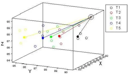
Figure 2.1: Example of a typical situation we are interested to investigate. In fig. 2.1 we have illustrated a situation we could be interested to investigate: in this case we have 20 statistical units, that are part of 5 different groups (different treatments or products), on which three variables (𝑋, 𝑌 and 𝑍) are relevated; the full-coloured points represent the real average values of the three variables for each group, the empty-coloured points represent the observations and the circled point on the top is the optimum point, that rep-resents the whole of values that the average values should assume in order to have the best treatment of all. So, it should be clear that the less a medium point of a group is near the optimum point, the better that group is; as a result, in the example of the figure the true ranking of the 5 groups is: black ≻ red ≻ green ≻ blue ≻ yellow.
The topic of defining a treatment ranking from a multivariate point of view seems to be quite recent: it has been firstly addressed by Bonnini, Corain, Salmaso et al. in 20061 and the reference framework is experimental design
and analysis of variance. The literature of multiple comparison methods addresses the problem of ranking the treatment groups from worst to best, however there is no clear indications on how dealing with the information
from pairwise multiple comparisons, especially in case of blocking (or strati-fication) or in case of multivariate response variable.
This problem is not only of theoretical interest but it has also a recognized practical relevance, especially for applied research. Moreover, in industrial research a global ranking in terms of performance of all investigated prod-ucts/prototypes is very often a natural goal; as a proof, in 2008 an interna-tional industrial organization called AISE has formally incorporated such a method as official standard for industrial research on house cleaning prod-ucts2.
2.2
Theoretical background
2.2.1
The ANOVA model
Let Y be the multivariate numeric variable related to the response of any experiment of interest and let us assume, without loss of generality, that high values of each Y univariate element correspond to better performance and therefore to a higher degree of treatment preference. The experimental design of interest is defined by the comparison of 𝐶 groups or treatments with respect to 𝑆 different variables where n replications of a single experiment are performed by a random assignment of a statistical unit to a given group. The C-group multivariate statistical model (with fixed effects) can be represented as follows:
𝑌𝑖𝑗𝑘= 𝜇𝑖𝑗 + 𝜀𝑖𝑗𝑘, 𝜀𝑖𝑗𝑘 ∼ IID(0, 𝜎2𝑖𝑗), 𝑖 = 1, ..., 𝐶; 𝑗 = 1, ..., 𝑆; 𝑘 = 1, ..., 𝑛;
(2.1) where, in the case of a balanced design, n is equal to the number of replica-tions and indexes i and j are related with the groups (treatments) and the univariate response variable respectively.
The resulting inferential problem of interest is concerned with a set of 𝑆 hy-pothesis testing procedures 𝐻0𝑗 : 𝜇1𝑗 = 𝜇2𝑗 = . . . = 𝜇𝐶𝑗 vs. 𝐻1𝑗 : ∃𝜇𝑖𝑗 ∕= 𝜇ℎ𝑗,
𝑖, ℎ = 1, . . . , 𝐶, 𝑖 ∕= ℎ, 𝑗 = 1, . . . , 𝑆. If 𝐻0𝑗 is rejected a further possible set
of 𝐶 × (𝐶 − 1)/2 all pairwise comparisons are performed: {
𝐻0𝑖ℎ∣𝑗 : 𝜇𝑖𝑗 = 𝜇ℎ𝑗
𝐻1𝑖ℎ∣𝑗 : ∃ 𝜇𝑖𝑗 ∕= 𝜇ℎ𝑗
.
In the framework of parametric methods, when assuming the hypothesis of normality for random error components, the inferential problem can be solved by means of the ANOVA 𝐹 -test and a further set of pairwise tests using Fisher’s LSD or Tukey procedures, which are two of most popular multiple comparison procedures3. On the basis of inferential results achieved at the
univariate C-group comparison stage, the next step consists in producing a ranking of the treatments from the less to the more preferred.
2.2.2
5 proposed ranking methods
Scheme of ranking methods we are proposing
To perform almost all methods we are about to propose in the following subsubsections, we have to execute these steps:
1. the starting point is the result of the multiple comparisons analysis (𝑆 𝐶 × 𝐶 𝑝-value matrices);
2. a suitable score matrix is then defined;
3. through a synthesis procedure (sum, mean or some combination func-tion) the scores are synthesized into a 𝐶-dimensional score vector; 4. the set of 𝑆 score vectors are finally synthesized to perform one global
score vector4;
3See [36].
4We could also choose to use in the combining function different weights for the 𝑆
variables used to produce the score in order to give different levels of importance to them; in the 5 ranking methods we are presenting we will not use weights, or, if you want, we will use all weights equal to 1
5. the rank5 of this final global scores provides the required multivariate
global ranking of treatments.
We are about to present 5 ranking methods: three of them (AISE, NPC and GPS) are of particular scientific interest as we have already explained in the previous section and follow completely the scheme descripted above; the last two (Method “0” and Method “1”) are only used as terms of comparisons for the first three.
AISE score method
In 2007 Corain and Salmaso6 proposed to sum some meaningful scores from
inferential results at the univariate C-group comparison and then to apply the Non Parametric Combination (NPC) of partial rankings7. In this way
they acquire a unique preference criterion which jointly takes into account all performances achieved for every response variable. To illustrate the method, let us suppose H0𝑗 has been rejected for all 𝑗 = 1, ..., 𝑆, so that for each
uni-variate response there is some treatment that significantly differs for some others.
In order to suitably synthesize the pairwise comparison results for each re-sponse variable j, 𝑗 = 1, ..., 𝑆, let us define a set of 𝑆 score matrices of dimension 𝐶 × 𝐶, where each element [x𝑖ℎ∣𝑗] is related to the comparison
between the treatments i and h for each response variable j, giving the value of +1 to the significantly better treatment and −1 to the other, while both
5As we use rank transformation it is better to clear up that, from this moment and for
all this work, 1 is the worst treatment/product/group and 𝐶 is the best one, therefore with this choice the more the rank is high, the better the treatment is; this choice can appear a little strange, but we have done it essentially for two reasons: first because almost all scores are higher if the performance is better and lower if the performance is worse and second because the software we have used, R (see [39]), for default behaves like this.
6See [13]. 7See [29].
scores are 0 if the comparison is not significant. Formally, ⎧ ⎨ ⎩
if 𝐻0𝑖ℎ∣𝑗: 𝜇𝑖𝑗 = 𝜇ℎ𝑗 is not rejected then 𝑥𝑖ℎ∣𝑗 = 𝑥ℎ𝑖∣𝑗 = 0;
if 𝐻0𝑖ℎ∣𝑗: 𝜇𝑖𝑗 = 𝜇ℎ𝑗 is rejected then
{
if ¯𝑦𝑖𝑗 > 𝑦¯ℎ𝑗 then 𝑥𝑖ℎ∣𝑗 = +1 and 𝑥ℎ𝑖∣𝑗= −1;
if ¯𝑦𝑖𝑗 < 𝑦¯ℎ𝑗 then 𝑥𝑖ℎ∣𝑗 = −1 and 𝑥ℎ𝑖∣𝑗= +1;
(2.2)
where ¯𝑦𝑖𝑗 and ¯𝑦ℎ𝑗, 𝑖, ℎ = 1, . . . , 𝐶, 𝑖 ∕= ℎ, are the sample means of groups i
and ℎ for response variable Y𝑖𝑗, 𝑖 = 1, . . . , 𝐶, 𝑗 = 1, . . . , 𝑆. Note that
pair-wise comparisons and the valid score assignments are performed only when the 𝐶-sample test has rejected the null hypothesis 𝐻0𝑗, 𝑗 = 1, ..., 𝑆.
For each response variable 𝑗 = 1, ..., 𝑆 once this assignment has been per-formed for each pairwise comparison, it is easily feasible to obtain a set of 𝑆 𝑋𝑗 = [𝑥1∣𝑗, 𝑥2∣𝑗, . . . , 𝑥𝐶∣𝑗]′ score vectors, 𝑗 = 1, ..., 𝑆, where the 𝐶 elements
xi∣j , 𝑖 = 1, . . . , 𝐶, 𝑗 = 1, ..., 𝑆, of the score vector 𝑋𝑗, are calculated by
summing all the obtained scores for each treatment, i.e.: 𝑥𝑖∣𝑗 =
𝐶
∑
ℎ=1,ℎ∕=𝑖
𝑥𝑖ℎ∣𝑗, 𝑖 = 1, . . . , 𝐶, 𝑗 = 1, . . . , 𝑆. (2.3)
In order to obtain the final global AISE score we just apply a simple sum: 𝐴𝐼𝑆𝐸𝑖 =
𝑆
∑
𝑗=1
𝑥𝑖∣𝑗, 𝑖 = 1, . . . , 𝐶 (2.4)
In the end, we obtain the global combined ranking by applying the rank transformation:
𝐺𝐴𝐼𝑆𝐸𝑖 = 𝑅(𝐴𝐼𝑆𝐸𝑖) = #(𝐴𝐼𝑆𝐸𝑖 ≥ 𝐴𝐼𝑆𝐸ℎ), 𝑖, ℎ = 1, . . . , 𝐶. (2.5)
NPC score method
Instead of using ±1 summation as proposed by Corain and Salmaso in 2007, we could also make directly use of p-values. For this goal let us consider the set of 𝑆 one-sided p-value matrices of dimension 𝐶 × 𝐶, where each element
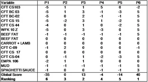
Figure 2.2: Example of calculation of AISE score for one variable.
Figure 2.3: Example of calculation of global AISE score (more than one variable).
[pih∣j] is related to the comparison between treatments i and h for response
variable j. For each response variable j, 𝑗 = 1, ..., 𝑆, it is possible to obtain an alternative set of 𝑆 score vectors 𝑋𝑗, 𝑗 = 1, ..., 𝑆, where each element of
𝑋𝑗 is calculated as follows: 𝑥𝑖∣𝑗 = −2 𝐶 ∑ ℎ=1,ℎ∕=𝑖 log(𝑝𝑖ℎ∣𝑗), 𝑖 = 1, . . . , 𝐶, 𝑗 = 1, ..., 𝑆. (2.6)
Note that we use as 𝑝-value synthesis criterion the Fisher’s combining func-tion. It is worth noting that the Fisher’s combining function is non-parametric with respect to the underlying dependence structure among 𝑝-values from different univariate response variables, in that all kinds of monotonic depen-dences are implicitly captured. Indeed, no explicit model for this dependence structure is needed and no dependent coefficient has to be estimated directly from the data.
Then, in order to suitably synthesize the scores for each response variable 𝑗, 𝑗 = 1, . . . , 𝑆, Corain and Salmaso suggested to use the Non-Parametric Combination (NPC) of partial rankings8 to acquire a unique preference
cri-terion which jointly takes into account all response variables. In order to obtain the final global NPC score we apply just a simple sum:
𝑁 𝑃 𝐶𝑖 = 𝑆
∑
𝑗=1
𝑥𝑖∣𝑗, 𝑖 = 1, . . . , 𝐶 (2.7)
In the end, we obtain the global combined ranking by applying the rank transformation:
𝐺𝑁 𝑃 𝐶
𝑖 = 𝑅(𝑁 𝑃 𝐶𝑖) = #(𝑁 𝑃 𝐶𝑖 ≥ 𝑁 𝑃 𝐶ℎ), 𝑖, ℎ = 1, . . . , 𝐶. (2.8)
GPS score method
With respect to each response variable an ANOVA test is performed and from the usual 𝐶 × (𝐶 − 1)/2 pairwise comparisons it is possible to test the statis-tical significance of the differences between the mean performances for each couple of treatments (𝑢, 𝑣). Let us indicate with 𝑦(1)𝑗 ≥ 𝑦(2)𝑗 ≥ . . . ≥ 𝑦(𝐶)𝑗 the ordered observed sample means for 𝑌𝑗 and assume that high values
cor-respond to better performance. The algorithm to calculate GPS score is the following:
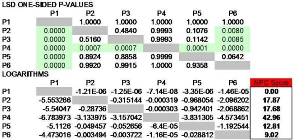
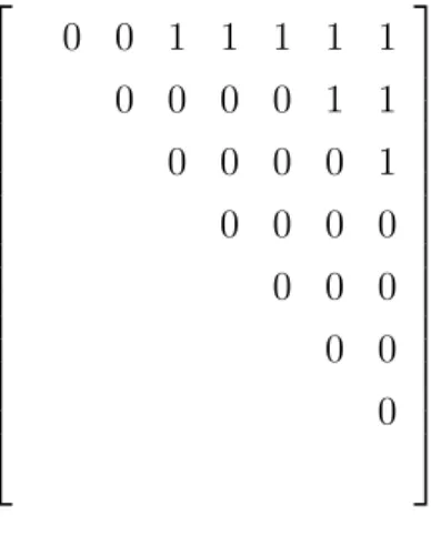
Figure 2.4: Example of calculation of NPC score (for one variable). 1. for each of the 𝑆 variables a 𝐶 ×𝐶 matrix 𝑋 is created (see the example
in table 2.1 at page 29) where the elements under the main diagonal are null and those over the main diagonal take value 0 or 1 according to the following rule:
𝑋[𝑢, 𝑣] = ℎ[𝑦(𝑢)𝑗, 𝑦(𝑣)𝑗] {
1 if 𝑦(𝑢)𝑗 is significantly not equal to 𝑦(𝑣)𝑗
0 otherwise;
(2.9) 2. a rank table, as shown in the example of table 2.1, is created according
to the following steps:
(a) in row 1, rank 𝐶 is assigned to the treatment with the higher mean (first column), indicated with (1), and to all the other products which mean performances are not significantly different from that of (1);
(b) in row 2, rank 𝐶 − 1 is assigned to the treatment with the higher mean, among those excluded from rank 𝐶 assignation, and to all the other products which mean performances are not significantly different from that of (2);
(c) in row 𝑟, rank 𝐶 − 𝑟 + 1 is assigned to the treatment with the higher mean, among those excluded from rank 𝐶 − 𝑟 assignation,
and to all the other products which mean performances are not significantly different from that of (𝑟);
(d) the iterated procedure stops when a rank is assigned to the prod-uct (𝐶);
3. for each treatment, the arithmetic mean of the values from the rank table (mean by columns) gives a partial performance score: 𝑥(𝑖)𝑗;
4. in order to obtain the final global GPS score we apply, as usually, just a simple sum: 𝐺𝑃 𝑆𝑖 = 𝑆 ∑ 𝑗=1 𝑥(𝑖)𝑗, 𝑖 = 1, . . . , 𝐶; (2.10)
5. in the end, we obtain the global combined ranking by applying, as usually, the rank transformation:
𝐺𝐺𝑃 𝑆
𝑖 = 𝑅(𝐺𝑃 𝑆𝑖) = #(𝐺𝑃 𝑆𝑖 ≥ 𝐺𝑃 𝑆ℎ), 𝑖, ℎ = 1, . . . , 𝐶. (2.11)
“0” method (mean of the means)
This is the first of the two methods we have used as terms of comparison for the previous three and it is very simple: it consists only in calculating the sample mean table (the mean of the variables in the different groups, so a 𝐶 × 𝑆 table) and then in aggregating with respect to the variables, simply by averaging and in this way obtaining a unique value for every group; the ranking is then obtained by applying the rank transformation to these values. In symbols operations made on observations 𝑦𝑖𝑗𝑘 are:
𝑦𝑖𝑗 = 1 𝑛 𝑛 ∑ 𝑘=1 𝑦𝑖𝑗𝑘, 𝑖 = 1, . . . , 𝐶; 𝑗 = 1, . . . , 𝑆; 𝑘 = 1, . . . , 𝑛. (2.12) 0𝑖 = 𝑦𝑖 = 1 𝑆 𝑆 ∑ 𝑗=1 𝑦𝑖𝑗 (2.13)
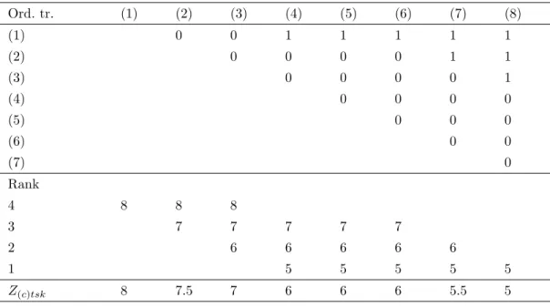
Ord. tr. (1) (2) (3) (4) (5) (6) (7) (8) (1) 0 0 1 1 1 1 1 (2) 0 0 0 0 1 1 (3) 0 0 0 0 1 (4) 0 0 0 0 (5) 0 0 0 (6) 0 0 (7) 0 Rank 4 8 8 8 3 7 7 7 7 7 2 6 6 6 6 6 1 5 5 5 5 5 𝑍(𝑐)𝑡𝑠𝑘 8 7.5 7 6 6 6 5.5 5
Table 2.1: Example of 𝑋 matrix for the multiple comparisons between pairs of products (𝐶 = 8).
𝐺0
𝑖 = 𝑅(0𝑖) = #(0𝑖 ≥ 0ℎ), 𝑖, ℎ = 1, . . . , 𝐶. (2.14)
This method is indeed based on no real score, but on two simple arithmetical means; anyway it can be seen as an application of Multicriteria Methods (see subsections 1.4.6 at page 16 and above all 3.2.2 at page 58).
“1” method (based on confidence intervals of distances)
This is the other method used as term of comparison, but this one is a little bit complicated, based on the distance between the observation and the optimum point, it consists in the following steps:
calculated for each unit9; 𝑑𝑖𝑘 = v u u ⎷ 𝑆 ∑ 𝑗=1 (𝑦𝑖𝑗𝑘− 𝑦𝑖𝑗𝑜)2 𝑖 = 1, . . . , 𝐶; 𝑗 = 1, . . . , 𝑆; 𝑘 = 1, . . . , 𝑛. (2.15) 2. arithmetic means of the distances are calculated, in order to obtain a unique value for every group (after this step we have a 𝐶-dimensional vector of means of distances);
𝑑𝑖 = 1 𝑛 𝑛 ∑ 𝑘=1 𝑑𝑖𝑘 (2.16)
3. from the vector of ordered means of distances confidence intervals10are
calculated and then a score 𝐶 × 𝐶 matrix 𝑋 of comparisons among groups is defined: 0 means that the two confidence intervals of that cell do intersect and therefore that the comparison is not significant, 1 means the contrary, that is the comparison is significant because the two intervals do not intersect; clearly, because of the ordering, the structure of matrix 𝑋 is very similar to the matrix used by GPS score (1s will be jointed on the top right and over the diagonal of the matrix, 0s will be elsewhere); the two limits of the confidence interval are:
𝑑1(𝑖) = 𝑑(𝑖)− 𝑡1−𝛼12 ; 𝑛𝐶−𝐶 𝑑2(𝑖) = 𝑑(𝑖)+ 𝑡1−𝛼12 ; 𝑛𝐶−𝐶 (2.17)
where 𝑑(𝑖) indicate the distances obtained at the previous step after we
have ordered them.
4. to 𝑋 GPS score for one variable is applied, in order to obtain a 𝐶-dimensional vector of scores: 1(𝑖);
9Notice that if we keep assuming that to large values correspond better performances
as we are doing (see the beginning of this section), to small (and not to large) distances correspond better performances.
10We suggest to use Bonferroni’s correction, in order to obtain simultaneous confidence
intervals, that simply consists in using a significance level that is the significance level declared (very often 0.05) divided for the number of comparisons we are going to do, that is(𝐶
5. afterwards the rank transformation is applied, but pay attention be-cause this is the only case where to lower scores correspond better per-formances and to higher scores correspond worse perper-formances, there-fore the rank transformation is applied indeed to the opposite values of the score (we mean for example −4 instead of 4):
𝐺1𝑖 = 𝑅(−1(𝑖)) = #(−1(𝑖) ≥ −1(ℎ)), 𝑖, ℎ = 1, . . . , 𝐶. (2.18)
Mean and variance of the proposed scores
For our future research on these topics and to inhance the evaluation of the results of simulations performed in this work, it is very useful to calculate mean and variance of the three scores of scientific interest, in order to obtain a way to better calculate11 confidence intervals of the scores. In fact the
scores defined by different procedures (both parametric and non-parametric) can be viewed as realizations of appropriate random variables and depending on hypothesis of random errors, the distribution of these random variables can be derived (parametrically or non-parametrically) in an exact or asymp-totically way.
AISE We have decided not to calculate mean and variance of AISE score because it would be not useful: as you will be able to see from the results of the simulation studies, it is clear that AISE score performs similar, but quite worse than GPS score and much worse than NPC score.
NPC In order to find a way to calculate mean and variance of NPC score, we have begun from this point12: under the null hypothesis 𝐻
0 (that is: “the
groups are all equivalent”) we have that 𝜓𝑖𝑗𝑘0 = −2
𝐶
∑
ℎ=1,ℎ∕=𝑖
log(𝑝𝑖ℎ∣𝑗) ∼ 𝑎𝜒2𝑔, 𝑘 = 1, . . . , 𝐵 (2.19)
11Better than those that we will use in our simulation studies, which are more
pseudo-confidence intervals of the scores than real true pseudo-confidence interval of the scores.
where 𝑎 is a parameter that takes into account the possible (probable in-deed) dependence between the components of the sum and if 𝑎 = 1 we have independence; 𝑔, instead, which represents the degrees of freedom of the chi-squared, is simply twice the number of components of the sum13; 𝑖
is the index of the group (𝑖 = 1, . . . , 𝐶), 𝑗 the one relative to the variable (𝑗 = 1, . . . , 𝑆) and, finally, 𝑘 is the index of the simulations (𝐵 is the number of them and normally we choose 𝐵 = 1000 or 𝐵 = 10000). Substantially we consider that sum, which synthesizes every simulation, the realization of a chi-squared variable modified with an appropriate multiplicative constant. So, we could think14 that, by adding a certain parameter 𝛿, we could report
the distribution under alternative hypothesis 𝐻1 to the one, simpler, under
𝐻0: 𝜓𝛿 𝑖𝑗𝑘1 = −2 𝐶 ∑ ℎ=1,ℎ∕=𝑖 log(𝑝𝑖ℎ∣𝑗) ∼ 𝑎𝜒2𝑔, 𝑘 = 1, . . . , 𝐵. (2.20)
Therefore, remembering properties of expectation and variance and that the mean of a chi-squared variable is its degrees of freedom and that the variance of a chi-squared variable is twice its degrees of freedom, we can state that:
𝐸(𝜓𝛿
1) = 𝑎𝑔 (2.21)
𝑉 𝑎𝑟(𝜓𝛿1) = 2𝑎2𝑔 (2.22)
And therefore a possible good estimation of parameter 𝑎 could be: ˆ 𝑎 = 1 2 ˆ 𝑉 𝑎𝑟(𝜓𝛿 1) ˆ 𝐸(𝜓𝛿 1) , (2.23) because: 𝑉 𝑎𝑟(𝜓𝛿 1) 𝐸(𝜓𝛿 1) = 2𝑎 2𝑔 𝑎𝑔 = 2𝑎. (2.24) 13Therefore 𝑔 = 2(𝐶 − 1).
14This was an idea of Lehmann who applied this to the uniform variable: under
null hypothesis 𝑝-value is distributed as a 𝑈 𝑛𝑖𝑓 (0, 1) variable, so we could think that 𝑝𝛿∼ 𝑈 𝑛𝑖𝑓 (0, 1)); nobody and nothing forbids us to use the same trick with a statistic
With a simulation study it is obviously very simple to calculate ˆ𝐸(𝜓𝛿 1) and
ˆ 𝑉 𝑎𝑟(𝜓𝛿
1), good estimations of the true 𝐸(𝜓𝛿1) and 𝑉 𝑎𝑟(𝜓𝛿1).
In order to estimate 𝛿, probably we have to do it in a numeric way, for ex-ample by minimizing a loss function; maybe it is also possible to do it in another way but still more methodological research on this topic is needed. We could say that all the reasoning about the calculation of expectation and variance of NPC score is based on a semi-parametric estimate of a distribu-tion.
GPS It is important to begin this paragraph saying that our research was not enough to find a real method to calculate expectation and variance of GPS score, anyway until now we have reached a good point and we are working on it.
The first idea we had and we tried to follow, was to find a 𝐶 × 𝑄15 matrix 𝐴
that pre-multiplicated to the 𝑄-dimensional vector 𝑌 (that is the matrix of 0s and 1s written as a vector) becomes the 𝐶-dimensional vector of the scores (in the end we have always one score for every different group/treatment), in symbols:
𝐴𝑌 = 𝑆; (2.25)
this idea seemed to be good because elements of 𝑌 are almost all realizations of bernoullian variables and, for the central limit theorem, we could approxi-mate the whole vector to a multivariate normal distribution, so that it would be very simple to calculate approximated estimations of 𝐸(𝑆) = 𝐸(𝐴𝑌 ) and 𝑉 𝑎𝑟(𝑆) = 𝑉 𝑎𝑟(𝐴𝑌 ) by finding matrix 𝐴.
But there are lots of problems following this idea, so we have tried an-other way: let us take as example the score matrix of table 2.1 at page 29 (see fig. 2.2). As we have already said, we can consider the scores 𝑥𝑖𝑗, 𝑖, 𝑗 = 1, . . . , 𝐶 in the matrix as realizations of known causal variables:
𝑋𝑖𝑗 ∼ Ber(𝑝𝑖𝑗), or analogously 𝑋𝑖𝑗 ∼ Bin(1, 𝑝𝑖𝑗), (2.26)
⎡ ⎢ ⎢ ⎢ ⎢ ⎢ ⎢ ⎢ ⎢ ⎢ ⎢ ⎢ ⎢ ⎢ ⎢ ⎢ ⎣ 0 0 1 1 1 1 1 0 0 0 0 1 1 0 0 0 0 1 0 0 0 0 0 0 0 0 0 0 ⎤ ⎥ ⎥ ⎥ ⎥ ⎥ ⎥ ⎥ ⎥ ⎥ ⎥ ⎥ ⎥ ⎥ ⎥ ⎥ ⎦
Table 2.2: Beginning score matrix useful to get E and Var of the final GPS score.
where 𝑝𝑖𝑗 is the probability that the comparison between group 𝑖 and group
𝑗 is significant, therefore:
∙ we can estimate every 𝑝𝑖𝑗, 𝑖 = 1, . . . , 𝐶 − 1; 𝑗 = 𝑖 + 1, . . . , 𝐶, (so only
probabilities of the comparisons written in the beginning score matrix) with the 𝑝-value of that comparison;
∙ where scores are not written, we can consider them to be always 0, so 𝑝𝑖𝑗 = 0, 𝑖 = 1, . . . , 𝐶; 𝑗 = 1, . . . , 𝑖; in this way on and below the
diag-onal of the matrix we can consider to have realzations of a degenerate variable.
Notice that now we can estimate expectation and variance of these 𝐶 × 𝐶 scores, remembering that for a bernoullian variable 𝑋 with parameter 𝜃, 𝐸(𝑋) = 𝜃 and 𝑉 𝑎𝑟(𝑋) = 𝜃(1 − 𝜃).
At this point we had the idea of transforming the beginning matrix in another one where written scores and scores on the diagonal are inverted (1 appears instead of 0 and viceversa) and the other not written scores are considered to stay equal to 0; therefore in our guiding example the matrix would become the one you can see in table 2.3:
⎡ ⎢ ⎢ ⎢ ⎢ ⎢ ⎢ ⎢ ⎢ ⎢ ⎢ ⎢ ⎢ ⎢ ⎢ ⎢ ⎣ 1 1 1 0 0 0 0 0 1 1 1 1 1 0 0 1 1 1 1 1 0 1 1 1 1 1 1 1 1 1 1 1 1 1 1 1 ⎤ ⎥ ⎥ ⎥ ⎥ ⎥ ⎥ ⎥ ⎥ ⎥ ⎥ ⎥ ⎥ ⎥ ⎥ ⎥ ⎦
Table 2.3: First passage matrix useful to get E and Var of the final GPS score.
Notice that even now we can estimate expectation and variance of the single scores: over the diagonal the probabilities of success and failure are now in-verted and are respectively 1 − 𝑝 and 𝑝.
Now in the first line we change 1 with 𝐶, in the second with 𝐶 − 1 and so on until the first line in which only 1s compare written16 and after that line
we write 0 in all last lines of the matrix; furthermore all 0s of the table are cancelled. So, in our example we have now the matrix you can see in fig. 2.4. Even now the moments of interest (E and Var) of the elements of this matrix can be simply estimated (we have to deal with bernoullian variables multi-plicated with some constants).
At this point we have some problems and we need some more methodolog-ical research to go on; we had thought two ways to obtain the vector of the 𝐶 scores, which in our example is indicated in fig. 2.5. The first way we had thought would be to find a certain 𝐶-dimensional vector, that post-multiplicated to the last calculated 𝐶 × 𝐶 score matrix (see table 2.4) should give the 𝐶-dimensional vector of scores, but this way seems not practicable at all. The second way would be to obtain the final 𝐶 scores by averaging
⎡ ⎢ ⎢ ⎢ ⎢ ⎢ ⎢ ⎢ ⎢ ⎢ ⎢ ⎢ ⎢ ⎢ ⎢ ⎢ ⎣ 8 8 8 7 7 7 7 7 6 6 6 6 6 5 5 5 5 5 ⎤ ⎥ ⎥ ⎥ ⎥ ⎥ ⎥ ⎥ ⎥ ⎥ ⎥ ⎥ ⎥ ⎥ ⎥ ⎥ ⎦
Table 2.4: Second passage matrix useful to get E and Var of the final GPS score.
[
8 7.5 7 6 6 6 5.5 5 ]
′
.
Table 2.5: Final scores.
by column the scores of the last 𝐶 × 𝐶 matrix, taking into account only the scores which are different from 0 (so, only the written ones). For example the fourth score of the example above is 6, because 6 is the mean of the written values of the fourth column of the last score matrix, that are 5, 6 and 7 and the last one is 5, because in the last column only one 5 is written.
But where is there the problem in this second choice? Until now after all passages we have always obtained a score matrix which components are de-scriptable in terms of expectation and variance of the causal variables of which they are realizations, but on the final score vector it is very difficult to calculate expectation and variance, because we should calculate expecta-tion and variance of the ratio of two causal variables: in fact the final scores
𝑥𝑖, 𝑖 = 1, . . . , 𝐶 are calculated in this way: 𝑥𝑖 = ∑𝐾𝑖 𝑗=1𝑥˜𝑖𝑗 𝐾𝑖 ,
where ˜𝑥𝑖𝑗 are the scores of the last 𝐶 ×𝐶 matrix and 𝐾𝑖 is the causal variable
that describes the number of written values for the column 𝑖 of the matrix. Therefore we are now not able any more to go on and to calculate expecta-tion and variance of the final scores, but probably we are very close to our goal. We must also say that we have not already taken in account that if in the beginning score matrix we have two equal lines, we have to jump one of them and this can complicate the calculation of the moments during all passages we have illustrated.
Anyway the situation is not so bad, because the way of calculating the mo-ments of the most important score, NPC, is almost completely sketched out and with the calculation of the moments of GPS score, as we have just said, we are not so far to complete it with some more research.
2.3
Simulation study
In order to evaluate the degrees of accuracy of these methods in detecting the true “unknown” treatment ranking, in this section we will perform a first simulation study where parameters are set and errors are randomly gen-erated. In sections 2.5 and 3.3, respectively at pages 44 and 61, you will find other two simulation studies: the second uses true experimental data, the third is similar to the first, but contains some issues more than the first one. The main goals of these three simulation studies are to find out the best performing and the more robust multivariate ranking methods and to investigate the role played by the number of treatment to be ranked, the dimension of the response variable and the number of replications.
In these simulation studies we have applied the ranking methods (NPC, AISE, GPS) only to quantitative variables, but these methods are completely applicable also to qualitative variables, and in particular also ordinal
vari-ables (therefore also Likert’s scales): to adapt the three methods to ordinal variables it is enough to obtain 𝑝-values of comparisons with an appropriate test for ordinal variables, instead of 𝑡-test, because as we can obtain some 𝑝-values that describe the pairwise comparisons, than we are completely ca-pable to perform the three methods. It is very interesting that we can apply these methods also to ordinal variables and in particular to Likert’s scales, because it could be possible to use them in the analyses of questionnaires with Likert’s scales, analyses which we descripted in the first chapter. But, as we have already said, now we are going to deal only with quantita-tive variables, even if, results are extendable to other types of variables (the main point is using a correct test for the comparisons), and in this section we are dealing only with the first simulation study; let us consider the following simulation settings:
∙ 3 and 6 positive numeric response variables (𝑝 = 3, 6), with “hypothet-ical” maximum value at 100 (the optimum point);
∙ 3, 5 and 7 treatments (𝐶 = 3, 5, 7);
∙ 4 and 8 experimental replications (𝑛 = 4, 8);
∙ three types of random errors (𝜀𝑖𝑗𝑘, 𝑖 = 1, . . . , 𝐶; 𝑗 = 1, . . . , 𝑝; 𝑘 =
1, . . . , 𝑛): normal, skew-normal17 (with shape parameter equal to 5)
and Student’s t (with 2 degrees of freedom). We have chosen these three distributions in order to have good examples of: a symmetric distribution with light tails (low curtosis) (normal distribution), an asymmetric distribution (we wanted to use exponential distribution, but there were lots of difficulties in using it at a multivariate level, so we chose skew-normal distribution), a symmetric distribution with heavy tails (high curtosis) (Student’s t with 2 degrees of freedom);
17For further information on this finding of prof. Adelchi Azzalini of Department of
∙ three variance-covariance settings (different variance-covariance matri-ces (𝑝 × 𝑝) of the vectors of random errors):
1. setting 1: variables are independent (𝜎2
𝑖ℎ = 0, 𝑖, ℎ = 1, . . . , 𝑝, 𝑖 ∕=
ℎ) and their variances are homoscedastic (𝜎2
𝑖𝑖 = 1, 𝑖 = 1, . . . , 𝑝);
2. setting 2: variables are independent (𝜎2
𝑖ℎ = 0, 𝑖, ℎ = 1, . . . , 𝑝, 𝑖 ∕=
ℎ) and their variances are heteroscedastic (𝜎2
11 = 1, 𝜎222= 4, 𝜎332 =
2.25);
3. setting 3: variables are not independent (covariances are all dif-ferent with values in the interval [0, 1]) and their variances are homoscedastic (𝜎2
𝑖𝑖 = 1, 𝑖 = 1, . . . , 𝑝);
∙ the 𝑝 𝐶 × 𝐶 matrices of 𝑝-values are obtained with 𝑡-test: in NPC and AISE they are unilateral and no correction is applied, whereas in GPS they are bilateral and correction for multiple comparisons is applied18.
∙ 1000 independent simulations are performed for each of the 108 settings (2 × 3 × 2 × 3 × 3);
∙ fixed structures of true treatment mean values (see the two tables in the next page).
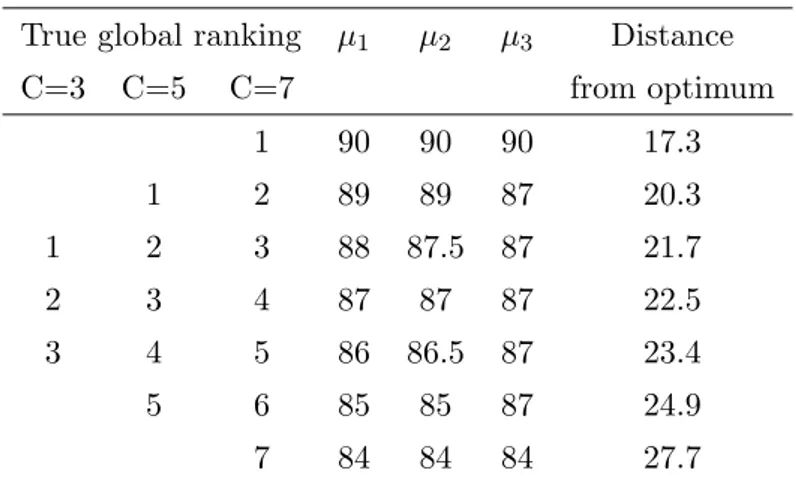
Note that the true global ranking follows the label treatment ordering and can be obtained by calculating the euclidean distance of each treatment from the perfect ideal treatment, that is from the 3-dimensional point (100, 100, 100) with 3 variables or from the 6-dimensional point (100, 100, 100, 100, 100, 100) with 6 variables.
True global ranking 𝜇1 𝜇2 𝜇3 Distance C=3 C=5 C=7 from optimum 1 90 90 90 17.3 1 2 89 89 87 20.3 1 2 3 88 87.5 87 21.7 2 3 4 87 87 87 22.5 3 4 5 86 86.5 87 23.4 5 6 85 85 87 24.9 7 84 84 84 27.7
Table 2.6: Setting of treatment mean value for simulation study (𝑝 = 3).
True global ranking 𝜇1 𝜇2 𝜇3 𝜇4 𝜇5 𝜇6 Distance
C=3 C=5 C=7 from optimum 1 90 90 90 90 90 90 24.5 1 2 89 89 87 90 89 89 27.4 1 2 3 88 87.5 87 90 87 87 30.1 2 3 4 87 87 87 87 87 87 31.8 3 4 5 86 86.5 87 84 87 86 34.2 5 6 85 85 87 84 85 84 36.8 7 84 84 84 84 84 84 39.2
Table 2.7: Setting of treatment mean value for simulation study with (𝑝 = 6).
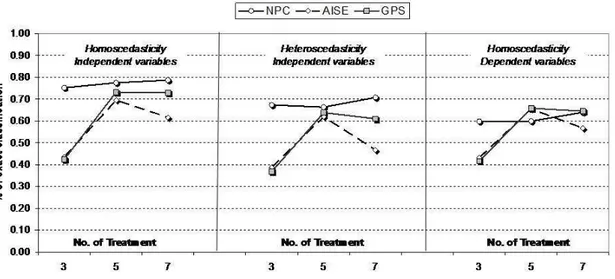
Analyzing results of this first simulation study (you can find an example19of
how we can present results in fig. 2.5) we can eventually state some consid-erations:
19In this first study we have performed only two indexes/calculations to analyze results
for every method for every setting: classification matrix and the percentage of simulations when Spearman’s 𝜌 calculated between the true ranking and the calculated ranking is equal to 1 (for further details on these indexes see the second simulation study); in the example of fig. 2.5 this percentage is 52.5 for NPC method, 19.7 for AISE method and 20.2 for GPS method.
Figure 2.5: First simulation study: example of results (classification matri-ces) in the setting with p=3, C=5, n=4, normal errors, indep.-heter. var.-cov. matrix.
Figure 2.6: First simulation study: example of results (rate of right classi-fication for the median treatment) in the settings with p=3, n=4, normal errors.
∙ the most performing method between those of interest is NPC, that is much better than AISE; GPS is almost in the middle of the two methods, but much less performing than NPC and not very distant from AISE; method “1” is completely wrong to search the true ranking (we could expect it because it is very difficult that confidence intervals