High resolution urban monitoring using neural network and transform algorithms

(1)

Universit`

a degli Studi di Roma

“Tor Vergata”

Dipartimento di Informatica, Sistemi e Produzione

Doctor of Philosophy PhD., Geoinformation

High Resolution Urban Monitoring Using Neural

Network and Transform Algorithms

Professore: Candidata:

Fabio Del Frate Chiara Solimini

Professore:

William J. Emery

(2)

A Maria, Giovanni e Rosaria che vivranno sempre nel mio cuore.

(3)

To A: “You must be the change you wish to see in the world.”

(4)

3.1.1 The Neural Net method: Performance and comparison with other method . . . 29 3.1.2 The Neural Network algorithm . . . 30 3.1.3 Single image classification: MLP near-optimal structure 32 4 Methods to “globally” characterize a (large) urban area 43 4.1 The Discrete Fourier Transform . . . 43

(5)

Index 5

4.1.1 The Discrete Spectrum . . . 43

4.1.2 Discrete Fourier Transform Formulae . . . 44

4.1.3 Properties of the Discrete Fourier Transform . . . 45

4.2 The Discrete Fourier Transform of an Image . . . 46

4.2.1 Definition . . . 46

4.2.2 Evaluation of the Two Dimensional, Discrete Fourier Trans-form . . . 47

4.2.3 The Concept of Wavenumber . . . 48

5 Applications 51 5.1 Detailed classification of “elementary” surfaces using the opti-cal/IR spectra . . . 51

5.2 Global characterization of large cities of parts of cities . . . 54

5.3 High Resolution Change Detection . . . 54

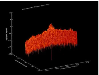
5.3.1 Transform algorithms to characterize urban areas . . . . 57

6 Conclusions 99

7 Acknowledgement 119

(6)

Chapter 1 Introduction

Urban areas occupy a relatively small portion of the earth surface. At the same time they represent one of the most complex, intricate, and variable of all land covers and land use and are also among the most rapidly expanding and changing elements of the landscape. A timely manner of monitoring urban areas is needed to be able to accurately assess the impact of human activi-ties on the environment; in particular, monitoring the existence, distribution and changing patterns of cities which play a crucial role in the allocation and conservation of natural resources, environmental and ecosystem management, and economic development. Also, an understanding the dynamics of the urban area and its impact of the human activities on the environment is needed to assess and to assess the supporting land carrying capacity. Usually land cover and classification maps are provided by government administration and field surveys, collecting, for example, aerial pictures and national censuses.

However, the data collection provided by these techniques is costly and time consuming, often not updated and lacking in detailed information. Real-istically, the only feasible source of information on land cover over large areas which allows data to be acquired in a regularly repeatable manner is satellite remote sensing. Indeed, in principle, remote sensing systems could measure

(7)

1. Introduction 7

ergy emanating from the earth’s surface in any reasonable range of wavelenghts (Richards (1993)). However, in spite of the great potential of remote sensing as a source of information on land cover and the long history of research devoted to the extraction of land cover information from remotely sensed imagery, many problems have been encountered, and the accuracy of land cover maps derived from remotely sensed imagery has often been viewed as too low for operational users (Bernard et al. (1997), Binaghi et al. (1996) and Foody (2002)).

Many factors may be responsible for these problems. These include the nature of the land cover classes (e.g. discrete or continuous), the properties of the remote sensor (e.g., its spatial and spectral resolutions), the nature of the land cover mosaic (e.g., degree of fragmentation), and the methods used to ex-tract the land cover information from the imagery (e.g., classification methods) (Foody and Ajay (2004)). These various problems have driven research into a diverse range of issues focused on topics such as image analysis techniques. Many of the problems in mapping land cover noted in the literature are asso-ciated with the methods used to extract the land cover information from the imagery. This has motivated a considerable amount of research into classifica-tion methods and supervised classificaclassifica-tions in particular. Early work based on basic classifiers such as the minimum distance to means algorithm prompted the adoption of more sophisticated statistical classifiers such as the maximum-likelihood classification. Problems associated with satisfying the assumptions required by such classification methods has driven research into nonparamet-ric alternatives including techniques such as evidential reasoning (Peddle and Franklin (1992), Wilkinson and Megier (1990)) and more recently neural net-works (Benediktsson et al. (1990), Kanellopoulos and Wilkinson (1997), Liu et al. (2003), and Del Frate et al. (1999)), decision trees (Goel et al. (2003), McIver and Friedl (2002) and Friedl and Brodley (1997)) and genetic algorithms (Nabeel et al. (2006)). Indeed, the accuracy with which land cover may be classified by these techniques has often been found to be higher than that

(8)

de-1. Introduction 8

rived from the conventional statistical classifiers (e.g. Peddle et al. (1994), Rogan et al. (2002), Li et al. (2003) and Pal and Mather (2003)).

The advent of the recent generation of very high spatial resolution satellites has lead to a new set of applications made possible by the geometrical preci-sion and high level of thematic detail in these images. In particular monitoring urban areas has captured the researchers attention. In fact, urban analysis using high spatial resolution involves a large number of applications such us road network mapping, government survey map updating, monitoring of ur-ban growth and over building. These kinds of applications were not feasible with the previous generation of moderate-resolution satellites (e.g. Landsat Thematic Mapper). However, further improvements in the accuracy of auto-mated classification algorithms are needed to satisfy the end-user requirements in all application domains. In particular, the number of classes extracted by classification algorithms is relatively low when compared with the number of-ten required by environmental mapping agencies to describe land cover uses at regional, national and continental scales (e.g. the European Environment Agency’s hierarchical CORINE Land Cover Data Set: 44 classes; the U.S. Na-tional Land-Cover Data 2001: 26 classes at level II). This lack of classification efficiency still leads to time consuming and expensive photointerpretation pro-cedures.

For these reasons, it is important that the remote sensing community in-vests more energy to define advanced and effective methods to address the classification problem. Thus, research into new classification methods contin-ues, and support vector machines (SVMs) have recently attracted the attention of the remote sensing community (Huang et al. (2002), Brown et al. (1999) and Halldorsson et al. (2003)). A key attraction of the SVM-based approach to im-age classification is that it seeks to fit an optimal hyperplane between classes and may require only a small training sample (Huang et al. (2002), Mercier and Lennon (2003) and Belousov et al. (2002)). Although the potential of

(9)

1. Introduction 9

SVM is evident and early studies have demonstrated considerable success in using them to map land cover accurately, there are problems in their usage (Foody and Ajay (2004)). One of the main concerns is that SVMs were origi-nally defined as binary classifiers and their use for multiclass classifications is problematic, requiring strategies that reduce the multiclass problem to a set of binary problems. Therefore, the researchers have sought to extend the basic binary SVM approach to form a multiclass classifier (Perez-Cruz and Artes-Rodriguez (2002), Angulo et al. (2003), Lee et al. (2003), Zhu et al. (2003)) and recently an approach for “one-shot” multiclass SVM classification has been reported (Hsu and Lin (2002)). However, at the present state of the art there is no discernible evidence in the classification accuracy advantages between the neural and non-neural approaches (Wilkinson (2005)).

In this context, one of the major problem related to high resolution image processing is to handle the extremely large set of data, therefore challenging, the general ability of the chosen classification algorithm. With respect to clas-sical methods, neural networks represent a fundamentally different approach to problems like pattern recognition. They do not rely on probabilistic assump-tions and do not need assumpassump-tions about normality in data sets. Moreover, they show a considerable ease in using multi-domain data sources. The effec-tiveness of neural networks is related to their self-adaptive characteristic; in particular, they can adjust themselves to the input data without any a priori assumptions (e.g., they do not require any explicit specification of the data dis-tribution), and can approximate any function with arbitrary accuracy (Bishop (1995)). Therefore, neural network algorithms are well suited to the classifica-tion of remote sensing images.

A crucial issue which the classification accuracy depends on, is the decision-making process related to the assignment of the classes (e.g, in a pixel based classification, to assign a pixel to one class rather than a different one). The class assignment process performed by a classifier based on neural network

(10)

al-1. Introduction 10

gorithms has been found to be effective (Del Frate et al. (1999), Del Frate et al. (2004)). For this reason Neural Networks (NN) have received considerable attention, as a tool in the field of remote sensing, after a new training scheme was developed. This new principle of a back-propagation algorithm was initially proposed by Werbos (1974) and rediscovered by Rumelhart et al. (1986). As explained above, since the early 1990s, several researchers have compared the performance of NN with conventional statistical approaches for remote sensing image classification. Benediktsson et al. (1990) evaluated the both methods for multi-source remote sensing data classification. They noted that a neural network has a great potential as a pattern recognition method for multi-source remotely sensed data due to its underlying distribution-free nature. Bishof et al.(1994), Paola and Schowengerdt (1995) compared methods for multispectral classification of Landsat TM data and both found that with proper training, a neural network was able to perform better than the maximum-likelihood classifier. However, even if these studies seem to show that NN performance is comparable or better than those provided by other techniques, they were mainly focused on medium resolution Landsat images and on the use of a sin-gle neural network for classifying and/or extracting specific features from a single image, namely the same image from which the examples training the network are taken.

A detailed analysis of the pixel-based classification yielded by this type of NN algorithm on very high resolution images such as those provided by the QuickBird (QB) or Ikonos platforms is still lacking. Moreover, the potential of a single neural network as a tool for automatic and sequential processing of images contained in high-resolution image archives has been scarcely investi-gated. With sequential processing we mean that the network might be able to retrieve from the archive all the images that contain or do not contain a specific class of land cover, or where the ratio between areas corresponding to different classes is within/out predefined ranges. In other words the NN allows the

(11)

iden-1. Introduction 11

tification of high-level (object or region of interest) spatial features from the pixel representation contained in a raw image or image sequence, hence being able to address scientific issues characteristic of the image information mining field (Datcu et al. (2003) and Hsu et al. (2002)).

As a first step, in this study, we want to assess and optimize the neural net-work approach for the pixel-based classification of a single very high resolution image, such as those provided by the QB satellite.

Next we move to the conceptually most innovative part of the study which is to investigate the capabilities of supervised NN in providing automatic classi-fication of a collection of images, therefore assessing their potentialities from an image information mining point of view. This stresses their general capabilities to adapt to new input patterns different from the patterns on which the nets have been trained. Several factors interfere with the objective of designing a NN able to be generalized for their use with images not used in the training phase. Examples the influences the different incidence angles and/or atmo-spheric conditions or the fact that different types of material may characterize the same class. In spite of these problems, the robustness of the spectral infor-mation has to be investigated and such an analysis needs to concur with the design of the NN. Addressing this point, we consider both very high (QB) and moderate (Landsat) resolution images and a specific application domain which is the feature extraction and information discovery applied to urban areas.

In fact, monitoring changes and urban growth over time is one of the major challenges of scientific research in remote sensing with a strong potential for the policy implications of this image analysis that would improve environment and security monitoring (Jensen and Cowen (1999), Donnay et al. (2001), Carlson (2003)). For example in Wilson et al. (2003) an urban growth model is devel-oped. The model, which is based on land cover derived from remotely sensed satellite imagery, determines the geographic extent, patterns, and classes of urban growth over time. Synthetic Aperture Radar(SAR) imagery can also be

(12)

1. Introduction 12

used, providing an additional source of information and enhancing the capabili-ties of optical data (Dell’Acqua et al. (2003), Schiavon et al. (2003)). Therefore a large volume of satellite data is available, but despite many competing auto-matic approaches, it is difficult to fully and autoauto-matically address the problems raised by the different application scenarios. In this study the aim of the clas-sification is to distinguish between areas of artificial cover (sealed surfaces) including asphalt or buildings, and open spaces such as bare soil or vegetation. As a by-product this makes possible the retrieval of other features such as the detection of new buildings or the discovery of modifications in existing ones.

1.1 Relevance of classification and change detection

in monitoring urban areas: evolution and

pro-cesses

Classification

Ever since the first multispectral imagery became available from civilian remote sensing satellites in the late 1970s, considerable effort has been devoted to the classification of image data with the aim of producing high-quality the-matic maps and establishing accurate inventories of spatial classes (Wilkinson (2005)). Classification is regarded as a fundamental process in remote sensing, which lies at the heart of the transformation from satellite image to usable geographic products. In order to produce thematic maps different methodolo-gies of image classification have been developed. In particular, we can separate classification methods by the following:

• the development of components of the classification algorithm including the training or learning strategy and approaches to class separation based on statistical or other estimators and class separability indexes,

(13)

1. Introduction 13

• the development of novel system-level approaches that augment the un-derlying classifier algorithms,

• the exploitation of multiple types of data or ancillary information, both numerical and categorical, in a classification process.

In the first category we can include the development of the supervised maximum-lakelihood method (Frizzelle and Moody (2001), Benediktsson et al. (1990)), n-dimensional probability density function methods (Cetin et al. (1993)), artificial neural networks (Gamba and Houshmand (2001), Yoshi and Omatu (1994), Bishof et al. (1994), Heerman and Khazenie (1992), Atkinson and Tatnall (1997), Paola and Schowengerdt (1995), Serpico and Roli (1995), Kanellopoulos and Wilkinson (1997), Ji (2000) and Dreyer (1993)), decision trees (Hansen et al. (1996), Kumar and Majumder (2001)), discriminant anal-ysis (Franklin (1994), Hardin (1994)), genetic algorithms (Tso and Mather (1999),Sheeren et al. (2006)) and spectral shape analysis (Carlotto (1998)). In the second category we includ fuzzy or similar approaches that “soften” the results of a hard classifier (Seong and Usery (2001), Foody (1996), Foody (2002), Zhang and Foody (1998), Bastin (1997), Du and Lee (1996)), mul-ticlassifier systems that integrate the outputs of several underlying classifier algorithms (Wilkinson et al. (1995)), and decision fusion methods (Benedikts-son and Kanellopoulos (1999), Jimenez et al. (1999), Petrakos et al. (2001)).

The third category includes the use of texture measures extracted from im-agery (Franklin et al. (2001), Augusteijn et al. (1995)), the use of structural or spatial context information from the imagery (Barnsley and Barr (1996),Gong and Howarth (1990)), the use of multisource data (Bruzzone et al. (1997), Bruz-zone et al. (1999), Zhang (2001)), and the use of ancillary geographical knowl-edge integrated in the overall classification system through, for example, an ex-pert system approach (Srinivasan and Richards (1990), Moller-Jensen (1990), Wilkinson and Megier (1990), Kontoes et al. (1993), Tonjes et al. (1999)). Some

(14)

1. Introduction 14

approaches integrate several of the afore-mentioned, e.g., (Debeir et al. (2002)).

Change Detection

Detection of land-cover changes is one of the most interesting aspects of the analysis of multitemporal remote sensing images (Richards (1993)). In partic-ular, change detection is very useful in many applications, like land use change analysis, assessment of burned areas, studies of shifting cultivation, assessment of deforestation etc. (Singh (1989), Coppin and Bauer (1994), Green et al. (1994)). Further, the recent availability of very high resolution images has en-larged the number of applications especially in urban monitoring such as the growth of urban areas and discovering building permit infractions (Bruzzone and Carlin (2006)). Usually, change detection involves a couple of spatially reg-istered remote-sensing images acquired of the same area at two different times. Two main approaches to detecting land-cover changes can be distinguished (Bruzzone and Serpico (1997)):

1. changes detected by comparing the spectral reflectances of multitemporal satellite images,

2. changes can be detected by using supervised classifiers.

Many change detection algorithms are based on the first approach (Singh (1989), Fung and LeDrew (1987), Chavez and MacKinnon (1994), Muchoney and Haack (1994), Fung (1990), Muchoney and Haack (1994)). The Univariate Image Differencingalgorithm (Singh (1989), Fung (1990), Chavez and MacK-innon (1994), Muchoney and Haack (1994)) performs change detection by sub-tracting, on a pixel basis, the images acquired at two times to produce a “differ-ence image”. Under the hypothesis that there are only minor changes between the two times, changes can be detected in the tails of the probability density functions of the pixel values in the difference image; this technique is usually

(15)

1. Introduction 15

applied to a single spectral band. Other techniques, like Vegetation Index Dif-ferencing(Singh (1989), Townshend and Justice (1995)) make the same kind of comparison by using, instead of a spectral band, vegetation indices (Richards (1993)) or other linear (e.g., Tasseled Cup Transformation (Richards (1993), Fung (1990))) or nonlinear combinations of original satellite bands. The widely used Change Vector Analysis technique (Singh (1989)) exploits a similar con-cept. In this case, however, the pixels at each time are represented by their vectors in the feature space. Then, for each couple of pixels, the “spectral change vector” is computed as the difference between the image feature vectors at the two times. The statistical analysis of the magnitudes of the spectral change vectors allows one to detect the presence of changes, while their direc-tions make it possible to distinguish between different kinds of transidirec-tions.

Another technique similar to those described above is Image Rationing; in this case, the comparison between spectral bands at two times is performed by computing the ratio, instead of the difference, between images. Techniques based on Principal Component Analysis (Singh (1989), Fung and LeDrew (1987), Muchoney and Haack (1994)) can also be used to perform change detection by applying the principal component transformation separately to the feature space at each time or as to the merged feature space at two times. In the first case, change detection is performed with Vegetation Index Differencing using principal components instead of vegetation indices. In the second case land-cover changes are detected by analyzing the minor components of the transformed feature space (Singh (1989)). The above techniques usually do not aim to identify explicitly what kinds of land-cover transitions have taken place in an area (e.g., the fact that a vegetated area has been urbanized). Only the Change Vector Analysis technique allows one to distinguish among differ-ent kinds of land cover changes but, not being supervised, it does not explicitly identify the specific typologies of transitions. The above techniques are suitable for applications like, the definition of burned areas, the detection of pollution,

(16)

1. Introduction 16

deforestation, etc. However, they cannot be applied when the information on change character is not sufficient, like, for example, in the monitoring of chang-ing cultivation, where it is necessary to recognize the kinds of changes that have taken place in the agricultural area investigated. In addition, the performances of such technique is generally degraded by several factors like:

• differences in illumination at two times,

• differences in atmospheric conditions, in sensor calibration and in ground moisture conditions,

that make difficult a direct comparison between the raw images acquired at different times.

To overcome these problems, one can use the techniques based on a su-pervised classification of multitemporal images (Singh (1989)). The simplest technique in this category is Post-Classification Comparison (Singh (1989)). It performs change detection by comparing the classification maps obtained by in-dependently classifying two remote-sensing images of the same area acquired at different times. In this way, it is possible to detect changes and to understand the kinds of transitions that have taken place. Furthermore, the classification of multitemporal images avoids the need to normalize for atmospheric condi-tions, sensor differences etc., between the two acquisitions. However, the per-formances of the Post-Classification Comparison technique critically depend on the accuracies of the classification maps. In particular, the final change detection map exhibits an accuracy close to the product of the classification accuracies yielded at the two times (Singh (1989)). This is due to the fact that Post-Classification Comparisondoes not take into account the dependence ex-isting between two images of the same area acquired at two different times.

Supervised Direct Multidata Classification, (Singh (1989)), is able to over-come this problem. In this technique, pixels are characterized by a vector obtained by “stacking” the feature vectors related to the images acquired at

(17)

1. Introduction 17

two times. Change detection is then performed by considering each transition as a class and by training a classifier to recognize the transitions. Appropriate training sets are required for the success of this method: the training pixels at the two times should be related to the same points on the ground and should accurately represent the proportions of all the transitions in the entire images. Usually, in real applications, it is difficult to have training sets with such char-acteristics. In general the approach based on supervised classification is more flexible than that based on the comparison of multitemporal image data. In addition to the already mentioned capability to explicitly recognize land-cover transitions and to reduce the effects of different acquisition conditions at two different times, it also allows us to perform change detection using different sensors at different times. This is a useful property when change detection on a large time difference has to be performed and available images are provided by different sensors. The spatial resolution plays a key role in urban monitoring related to the detection of fine-scale objects present in urban scenes. In partic-ular high spatial resolution is required to reduce the problem of mixed pixels (i.e. the pixels that represent the spectral signature of more than one class due to the insufficient spatial resolution of the sensor) present in the medium res-olution images (e.g. Landsat imagery). Also the multispectral information is required to discriminate between the different surfaces/materials that compose the urban areas.

1.2 Type of surfaces to be classified

Since the appearance of very high resolution sensors and the object-oriented image analysis (OOIA), new questions about the acquisition of knowledge for classification procedures can be posed. The OOIA approach is characterized by the extraction of object primitives from images where each object corre-sponds to a group of homogeneous pixels. The object recognition methods are

(18)

1. Introduction 18

generally based on the use of knowledge related to spectral, spatial and contex-tual properties (e.g. mean of spectral and textural values, shape, length, area, adjacency and inclusion relationship...) (Sheeren et al. (2006)). While there are several studies that compare object-oriented and pixel-based classification techniques (Rego and Koch (2003)), only few works focus on the development of the knowledge base used to recognize the objects. No urban objects dictio-nary or ontology exists to create the knowledge base. Most of the time, the knowledge is implicit and is held only by the domain experts. However, the experts are rarely able to supply an explicit description of the knowledge they use in their reasoning. Data mining techniques, such as genetic algorithms, can help to derive this knowledge and to extract classification rules automatically. These rules are intended to enrich an ontology in the urban remote sensing imagery domain (Sheeren et al. (2006)). The algorithm has been succesfully tested on a very high resolution QuickBird multi-spectral (MS) image of an ur-ban area. In this work we use the results obtained in the above study: we make the assumption that the spectral signatures allows us to separate, at the first hierarchical level, these basic “elementary” classes, such as: vegetation, bare soil and “mineral”. The second hierachical level includes the segmentation of “mineral” surfaces into “man made” elements such as roads and buildings. Fi-nally, in the third hierachical level the “man made”surfaces are subdivided into residential, commercial, industrial etc.

(19)

Chapter 2 Remote Sensing Data

2.1 Optical/IR and radar available today and in near

future

Airborne and satellite remote sensing techniques have been investigated for human settlement detection, population estimation, and urban analysis since the mid-1950s (Henderson and Xia (1997)). Systems operating in the visible and near-infrared regions of the electromagnetic spectrum have received most of the attention and thus offer the most advanced and widely employed tech-niques. Starting in the early 1980s airborne imaging radar systems have also been used for urban land cover mapping, and offer some distinct advantages over optical sensors as well as contributing to potential synergistic benefits of merged data set. In fact, the reflectance measurements acquired in visible and infrared regions of the spectrum, are primarily related to molecular reso-nances of surface materials and visible radiometers are not able to sense the surface, under adverse meteorological conditions and during the night. The radar backscattering measurements are primarily related to the physical prop-erties of surface objects such as surface roughness and the dieletric constant. In particular, in a built up area, a radar backscatter signal depends on the

(20)

2. Remote Sensing Data 20

entation of facets and on the presence of dihedral corner reflectors, formed by the intersection of horizontal and vertical built features, and trihedral corner reflectors, formed by two orthogonal vertical walls and the ground (Schiavon and Solimini (2000)). Moreover, the radar sensor is able to collect data under all meteorological conditions and at any time of the day. However, the urban landscape is highly variable and complex and the radar signal interaction with the urban built-up area is not easy to interpret. Recently, modelling returns from urban structures have been carried out using L-band images of groups of buildings at linear polarizations and different incidence angles (Schiavon et al. (2001)).

Satellite Source Launch Sensors Types No.of Resolution

Name Channels (meters)

ERS-2 ESA 1995 AMI Radar 1 26

RADARSAT-1 Canada 1995 SAR Radar 1 9, 100

Lansat-7 US 1999 ETM+ MS

6 30

1 60

PAN 1 15

ROCSAT-1 Taiwan 1999 n/a

MS n/a 2

PAN n/a 8

IKONOS SpaceImaging 1999 IKONOS

MS 4 4

PAN 1 1

EROS-A1 ImageSat 2000 PAN PAN 1 1.5

Table 2.1 - Earth Observation Satellites: optical/IR and radar current missions. Satellites launched between 1995-2000.

(21)

QuickBird DigitalGlobe 2001

MS MS 4 2.44

PAN PAN 1 0.61

MTI US 2001 MTI MS 15 5

Envisat-1 ESA 2002 ASAR Radar 1 30, 150

SPOT-5 France 2002 HRV MS 3 10 1 20 PAN 1 2.5, 5 OrbView-3 Orbimage 2003 Orbview MS 4 4 PAN PAN 1 1 ROCSAT-2 Taiwan 2004 MS MS 4 8 PAN 1 2

IRS-P6 India 2004 LISS 3/4 MS 7 5.8, 23.5

ALOS Japan 2004

PALSAR Radar 1 10, 100

AVNIR-2 MS 4 10

PRISM PAN 1 2.5

EROS-B1 ImageSat 2004 PAN PAN 1 0.82

IRS-P5 India/US 2005 PAN PAN 1 2.5

KOMPSAT-1 Korea 1999 EOC PAN 1 6.6

KOMPSAT-2 Korea 2006

PAN PAN 1 1

MS MS 4 4

IRS-P5 India-US 2005 PAN PAN 1 2.5

CARTOSat-2 India-US 2005 PAN PAN 1 2.5

Table 2.2 - Earth Observation Satellites: optical/IR and radar current missions. Satellites launched between 2001-2005.

(22)

2.2 Relevance of Very-High-Resolution (VHR)

op-tical data

Remote sensing data with spatial resolutions of 0.5 − 10 m are required to adequately define the high wavenumber detail which characterizes the urban scene. This level of spatial resolution corresponds to scales between 1 : 10, 000 and 1 : 25, 000 (ignoring the effects of relief distortion etc.), that are typical of projects dealing with urban planning (Donnay et al. (2001)). The use of very high resolution (VHR) images, however, brings with it some major problems:

1. the majority of the highest resolution images are presently recorded in panchromatic mode only,

2. the corresponding large data set creates difficulties in terms of image storage, data exchange and processing time.

The first problem could be solved by using different data fusion techniques, i.e. merging the higher resolution panchromatic data with lower resolution multispectral data (Ackerman (1995), Jones et al. (1991), Wald et al. (1997)). Transforms in the color space (RGB/HSI), principal components analysis, spa-tial filtering and wavelets methods are among the most common means of achieving such integration (Carper et al. (1990), Chavez and et al. (1990) and Pohl and Van Genderen (1998)). Data fusion methods are also suitable for processing merged data sets involving sensors with different spatial resolutions and physical measurements such as radar and optical system (Schiavon et al. (2003)). This synergy can expand the optical system limits and improve the relatively poor spectral information related to the high-resolution data and im-prove the classification accuracy. In fact, in non-urban areas, it is generally possible to derive relatively direct relationships between the spectral responses in the four MS bands of natural components such as water, vegetation and soil and the measured image pixels reflectance values. In urban area,

(23)

identi-2. Remote Sensing Data 23

cal spectral reflectance values correspond to very different surface structures in terms of materials and fabrics, complicates the feature extraction process and the final output map.

The problems concerning the volume of data might appear of secondary im-portance given the rapid and continuing improvements in computer technology. Nevertheless, they remain significant at the scale of the urban region (typically several tens of square kilometers) and they necessitate the consideration of data compression techniques. In this context, wavelet and other transform methods are promising avenues of research. They not only allow efficient data compres-sion while preserving the original spectral values, but they can also be used to fuse images at different resolutions, thereby simultaneously dealing with the two main problems outlined above.

2.3 Features of data available today

Satellite Source Launch Sensors Types No.of Resolution

Name Channels (meters)

RADARSAT-2 Canada 2007 SAR Radar 1 3

CARTOSat-2 India-US 2007 PAN PAN 1 1

EROS-B2 ImageSat 2007 PAN PAN 1 0.7

EROS-C ImageSat 2008

PAN PAN 1 0.7

MS MS n/a 2.8

WorldView-1 DigitalGlobe 2007 PAN PAN 1 0.5

TerraSAR-X Germany 2007 SAR Radar 1 1

Table 2.3 - Earth Observation Satellites: optical/IR and radar future missions. Satellites missions for 2007 and later.

(24)

Chapter 3 Classification Methods of

High Resolution Remote

Sensing Data

As discussed in 2.2 Supervised classification is the procedure most often used for quantitative analysis of remote sensing image data. It is based on using suitable algorithms to label pixels in an image representing particular ground cover types, or classes. A variety of algorithms is available for this analysis, ranging from those based on probability distribution models for the classes of interest to those in which the multipsectral space is partitioned into class-specific regions using optimally located surfaces. Irrespective of the particular method chosen, the essential practical steps are:

• Decide the set of ground cover types into which the image is to be sub-divided. These are the information classes, for example, water, urban regions, vegetated areas, etc.

• Choose representative pixels for each of the desired classes. These pixels form the training set. Often the training pixels for a given class are in

(25)

3. Classification Methods of High Resolution Remote Sensing Data 25

a common region enclosed within a border often called the Region of Interest (ROI);

• Use the training data to estimate the values of the particular classifier algorithm to be used; these parameters will be the properties of the prob-ability model used to define partitions in the multispectral space. The set of parameters for a given class is sometimes called the signature of that class;

• Using the trained classifier, label or classify every pixel in the image into one of the desired ground cover types (information classes). Here the whole image is classified;

• Produce tabular summaries (typically the confusion or accuracy matrices) and thematic or classification maps which summarise the results of the classification.

In the recent literature, many papers have addressed the development of novel techniques for the classification of high resolution remote sensing images. In (Unsalan and Boyer (2004)), the authors present a technique for the identifi-cation of land developments over regions. The proposed technique uses straight lines, statistical measures (length, orientation, and periodicity of straight line), and spatial coherence constraints to identify three classes, namely 1) urban; 2) residential; 3) rural. In (Shackelford and Davis (2003)), a standard maximum-likelihood classifier is used to discriminate four spectrally similar macroclasses. Subsequently, each macroclass can be hierarchically subdivided according to class-dependent spatial features and a fuzzy classifier.

The main problem of these techniques is that they are highly problem de-pendent. This means that they cannot be considered as a general operational tool. In (De Martino et al. (2003)), the authors analyze the effectiveness of the gray-shade co-occurrence matrix (GLCM) texture features in modeling the

(26)

spa-3. Classification Methods of High Resolution Remote Sensing Data 26

tial context that characterizes high-resolution images. The fact that the analy-sis depends on the sample window and different heuristic parameters along with the intrinsic inability to model the shape of the objects leads to unsatisfactory classification accuracies. A more promising family of approaches for the anal-ysis of high resolution images is inspired by the behaviour of the human vision system, is based on an object-oriented analysis and/or multilevel/multiscale strategies. In these approaches each image is made up of interrelated objects of different shapes and sizes. Therefore, each object can be characterized with shape, topological measures, and spectral features. Objects can be extracted from images according to one of the standard segmentation techniques proposed in the literature (Haralick and Shapiro (1985)). The main idea of this multi-level analysis is that for each multi-level of detail, it is possible to identify different objects that are peculiar to that level and should not appear in other levels. In other words, each object can be considered to be its “optimal” representation level. Moreover, other aspects considered in this analysis are: 1) that objects at the same level are logically related to each other and 2) that each object at a generic level is hierarchically related to those at higher and lower levels (Binaghi et al. (2003), Benz et al. (2004), Burnett and Blaschke (2003)).

For example, in the multiscale analysis of a high resolution image, using the highest resolution, we can identify houses, gardens, streets, and single trees; at moderate levels, we can identify urban aggregates, group of trees, and agri-cultural fields; finally, at the coarsest level, we can identify towns and cities, forests, and agricultural areas as single objects. The exploration of the hierar-chical tree results in a precise analysis of the relations between these objects. For example, we can count the number of houses that belong to a specific urban area (Benz et al. (2004)). In (Binaghi et al. (2003)), the authors pro-pose an approach based on the analysis of a high-resolution scene through a set of concentric windows. The concentric windows analyze the pixel under investigation and the effects of its neighbors at different resolutions. To reduce

(27)

the computational burden, the information contained in each analysis window is compressed using a Gaussian pyramidal resampling approach. The classi-fication task is accomplished by a soft multilayer perceptron neural network that can be used adaptively as a pixel-based or an area-based classifier. One of the limitations of this approach is the fixed shape and choice of the analy-sis window size. In (Shackelford and Davis (2003)), an object-based approach is proposed for classification of dense urban areas from pan-sharpened multi-spectral Ikonos imagery. This approach exploits a cascade combination of a fuzzy-pixel classifier and a fuzzy object-based classifier. The fuzzy pixel-based classifier uses spectral and simple spatial features to discriminate between roads and buildings, which are spectrally similar. Subsequently, a segmented image is used to model the spectral and spatial heterogeneities and to improve the overall accuracy of the pixel-based thematic map. Shape features and other spatial features (extracted from the segmented image) as well as the previously generated fuzzy classification map are used as inputs to an object-based fuzzy classifier.

In (Benediktsson et al. (2003)), morphological operators are exploited within a multi-scale approach to provide image structural information for automatic recognition of man made structures. In greater detail, the structural informa-tion is obtained by applying morphological operators with a multi-scale ap-proach and analyzing the residual images obtained as a difference between the multiscale morphological images successive scales. A potential problem with this technique is the large feature space generated by the application of a series of opening and closing transforms. In (Benediktsson et al. (2003)), the authors overcome this problem by proposing the use of different feature-selection algo-rithms. An adaptive and supervised model for object recognition is presented in (Binaghi et al. (2003)), where a scale-space filtering process models and a multi-scale analysis for feature extraction is integrated to a unified framework within a multilayer perceptron neural network. This means that the error

(28)

back-3. Classification Methods of High Resolution Remote Sensing Data 28

propagation algorithm used to train the neural network also identifies the most adequate filter parameters. The main problems of this technique are related to the choice of the number and type of filters to be used in the input filtering layer (first layer) of the neural network.

In (Mott et al. (2002)), an algorithm based on selective region growing is proposed to classify a high-resolution image. In the first step, the image is classified by taking into account only spectral information. In the second step, a classification procedure is applied to the previous map by taking into account not only spectral information but also a pixel distance condition to aggregate neighboring pixels. By iteration, neighbor pixels that belong to the same class grow in a selective way, obtaining a final classification map. Nevertheless, as mentioned before, the few techniques specifically developed for the automatic analysis of high resolution images (compared with the abundant literature on the classification of moderate-resolution sensors), do not exhibit sufficient ac-curacy to satisfy the the end-user requirements in all application domains.

3.0.1 Unsupervised Neural Network Classification Algorithms: The Self-Organizing Map

In the context of the Unsupervised classification algorithms using NN, it is worthwhile to highlight the Self-Organizing map. Among the architectures and algorithms suggested for artificial neural networks, the Self-Organizing Map has the special property of effectively creating spatially organized “internal repre-sentation” of various features of input signals and their abstractions (Kohonen (1990)). Neighboring cells in a neural network compete in their activities by means of mutual lateral interactions, and develop adaptively into specific de-tectors of different signal patterns. In this case, learning is called competitive, unsupervised or self-organizing. The Self-Organizing Map is a sheet-like neural network, the cells of which becoming specifically tuned to various input signal

(29)

patterns or classes of patterns through an unsupervised learning process. The locations of the responses tend to become ordered as if some meaningful coor-dinate system for different input features were being created over the network. The spatial location or coordinates of a cell in the network then correspond to a particular domain of input signal patterns. Each neuron or local neuron group acts like a separate decoder for the same input. It is thus the presence or absence of an active response at that location, and not the exact input-output signal transformation or magnitude of the response, that provides an interpretation of the input information. Due to their characteristics, the Self-Organizing Maps (SOMs) are suitable for pattern recognition problems (e.g. image classification). In particular, the training phase is very fast compared to the supervised NN training phase (i.e. an iterative procedure). The SOMs have been succesfully used in different application domains with QB images: e.g. for detection of “man made” structures and changes (Molinier et al. (2006)), and to distinguish different kind of asphalt surfaces (e.g. concrete etc.) (Del Frate et al.(2004)).

3.1 Summary of methods used for classification by

spectral radiances

3.1.1 The Neural Net method: Performance and comparison

with other method

The use of neural networks in remote sensing has often been found effective, since they can simultaneously handle non linear mapping for a multidimensional input space onto the output classes and can cope with complex statistical be-haviour (Dawson (1994)). Neural networks, in contrast to statistically-based classifiers, do not require an explicitly well defined relationship between the input and output vectors, since they determine their own input-output

(30)

rela-3. Classification Methods of High Resolution Remote Sensing Data 30

tions directly from a set of training data (Rumelhart et al. (1986)). There are numerous types of neural networks used in classifying remotely sensed data. The most commonly used NN is the Multi Layer Perceptron (MLP)(Lippman (1987)) which has been found to have the best topology for the classification and inversion problems (Hsu et al. (1992)), trained by the backpropagation (BP) algorithm (Del Frate et al. (2000)). Minimization of the error function can also be pursued by a scaled conjugate gradient algorithm (Bishop (1995)). This is a member of the class of conjugate gradient methods (general purpose second order techniques) that help to minimize goal functions of several variables. Sec-ond order indicates that such methods use the secSec-ond derivatives of the error function, while a first order technique (like standard back-propagation) only uses the first derivatives (Del Frate et al. (1999)).

3.1.2 The Neural Network algorithm

The results shown in the following sections are also published in (Del Frate et al.(2006)) and Appendix. NN models are mainly specified by the net topol-ogy and training rules (Lippman (1987)). The term topoltopol-ogy refers to the struc-ture of the network as a whole: the number of its input, output, and hidden layers and how they are interconnected. Among various topologies, multilayer perceptrons (MLP) have been found to have the best suited topology for clas-sification and inversion problems (Hsu et al. (1992)). These are feed-forward networks where the input flows only in one direction to the output, and each neuron of a layer is connected to all neurons of the successive layer but has no feedback to neurons in the previous layers. As far as the numbers of hidden layers and of their sub units are concerned, the topology providing the optimal performance should be selected. In fact, if the number of neurons is too small, the input-output associative capabilities of the net are too weak. On the other hand, this number should not be too large; otherwise, these capabilities might show a lack of generality being too tailored to the training set which

(31)

unecessar-3. Classification Methods of High Resolution Remote Sensing Data 31

ily increases the computational complexity of the algorithm. It turns out that a fair compromise can be found.

The number of hidden layers is another issue to be considered. It has been shown that networks having two layers of weights, i.e. one hidden layer of neurons, and one of sigmoidal hidden units can approximate arbitrarily well any functional continuous mapping, provided the number of hidden units is sufficiently large (Bishop (1995), Hornik et al. (1989)). However how much the inclusion of an additional hidden layer might improve the classification perfor-mance is still an open issue.

In this work we followed a rather heuristic approach. We systematically analyze the performance of the network varying either the number of hidden layers (one or two) or the number of hidden units and selecting the best topol-ogy on the basis of quantitative results. Once the network topoltopol-ogy is selected, the weight or strength of each connection has to be determined via learning rules to approximate an unknown input-output relation. These rules indicate how to pursue the minimization of the error function measuring the quality of the network’s approximation of the restricted domain covered by a training set (i.e., a set of input-output examples). A typical error function which can be considered in this context is the sum-of-squares error function (SSE) (Bishop (1995)), given by a sum over all patterns, and over all outputs, of the form:

SSE = N X n=1 c X k=1 {yk(xn, w) − tnk}2 (3.1)

Here yk(xn; w) represents the output of unit k as a function of the input

vector xn

and the weight vector w, N is the number of testing patterns, and c is the number of outputs. The quantity tn

k represents the target value for

output unit k when the input vector is xn

. In our case the minimization of the error function has been carried out using a scaled conjugate gradient (SCG) algorithm (Moller (1993)). This is a member of the class of conjugate gradient methods, general purpose second order techniques that help to minimize goal

(32)

functions of several variables.

It should be mentioned that most of the neural net simulations were pro-vided by the SNNS (Stuttgart Neural Network Simulator) package (Stuttgart Neural Network Simulator (1995)). For the specific purpose of our image clas-sification a training-set with a statistically significant number of pixels for each class has been generated. The training of the neural network has then been car-ried out by feeding it with pairs of vectors (patterns): the input vector contains the reflectances of the different channels of the multi-spectral image, the output vector contains the corresponding known class of the surface. To avoid satura-tion within the network it has been necessary to scale all the values of the input vectors in the range between −1 and 1. This is also helpful to mitigate single-image effects if pixels belonging to different single-images are included in the training set. At the same time, the component of the output vector corresponding to the true class has been set to 1 while the others go to 0. Once the NN have been trained, they have been used for the classification of new data not used in the training set. In the test phase, a competitive approach (winner-take-all) has been considered to decide on the final classification response.

3.1.3 Single image classification: MLP near-optimal structure

The first applications of NNs in satellite image classification (Benediktsson et al.(1990)) established an additional merit of their use compared to conven-tional approaches (e.g. Maximum Likelihood): the ability to easily incorpo-rate non-spectral ancillary information (e.g. topographic) into the classifica-tion process without violating any assumpclassifica-tion, and as previously showed, NN outperformed statistical classifiers on several occasions (Kanellopoulos et al. (1992)). Nevertheless, there is no exact solution to find the optimal topology, in terms of resulting classification accuracy, of a MLP, until today. There have been several heuristics, some developed in the context of remotely sensed im-age classification specifically (Kanellopoulos and Wilkinson (1997)), that could

(33)

be the basis for exploring more efficient topologies by trial and error. These rules of thumb insure that the topologies, and thus results attained, will not deviate much from optimum. However, when the classification results are ex-tracted there is always the uncertainty related to the topology used and the classification accuracy (e.g., another topology could yield superior accuracy). There is no guarantee that a near-optimal topology has been found to perform the classification. The difficult part in determining an optimum MLP topol-ogy lays in hidden structures identification i.e. the identification of the best number of hidden neurons for each layer. Currently, there exist two general categories of approaches, pruning or growing algorithms (Lauret et al. (2006)) on one side and heuristics, which give us the hidden structure as a function of the number of input and output nodes, on the other (Kanellopoulos and Wilkinson (1997)). In this work we use the growing method: nodes are added progressively, e.g. starting with a single hidden node, until performance can no longer be improved.

The QuickBird commercial remote sensing satellite provides images con-sisting of four multi-spectral (MS) channels with 2.4 m resolution and a single panchromatic (PAN) band with a 0.62 m resolution. The four MS bands col-lect data at red, green, blue, and near-infrared wavelengths, and the data in each band is stored with an 11-bit quantization. As previously discussed, the spatial resolution plays a key role in urban monitoring related to the ability to detect fine-scale objects present in urban scenes. In particular, high resolution is a requirement to reduce the problem of mixed pixels (i.e. the pixels that represent the spectral signature of more than one class due to the insufficient resolution of the sensor) present in the medium resolution images (e.g. Landsat imagery). However, the high resolution sensors have a limited spectral resolu-tion, depending on technical constraints, that further increase the classification problem (Schowengerdt (2002)) and often do not allow a complete characteri-zation of different roof types, having different spectral signatures. However, a

(34)

method developed exploiting only the Digital Number (DN) belonging to rep-resentative pixels of each class randomly selected on QB images, is accurate in terms of classification results.

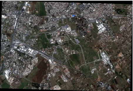
A QB image taken over the Tor Vergata University campus, located in Italy, South-East of Rome, on March 13, 2003, will be referred to as QB1. A view of the area obtained with the Red, Green and Blue bands is shown in Fig. 3.1.

Figure 3.1 -QuickBird image of the Tor Vergata University Campus, Rome, and its sour-rondings.

Besides the buildings of the campus, different residential areas belonging to the outskirts of the south-east side of the city can be distinguished in the image. Our first purpose was to design an optimum neural network able to classify the multi-spectral image. The land cover classes considered were build-ings, roads, vegetated areas, and bare soil where the latter class includes not asphalted road and artificial excavations. The inclusion of additional classes was discarded for several reasons: the considered classes are those that best describe the area under consideration and are in themselves sufficient to detect significant features. The choice of a small number of classes enables a more

(35)

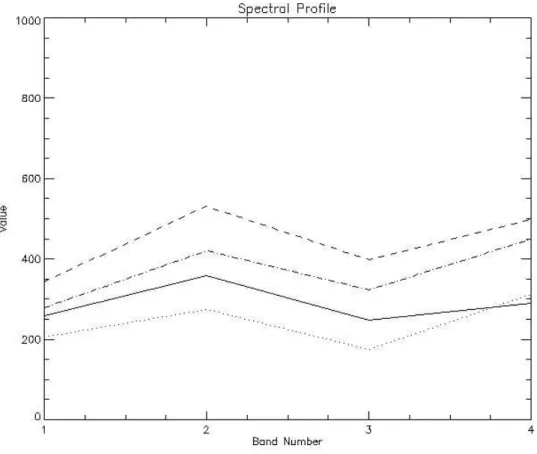
quantitative comparison of the performance obtained using a single net for a single image classification compared to the use of a single net for multiple im-age classification. In this latter case we think that the choice of a number of 4 classes represents a rather ambitious target. It also has to be noted that a recent study analysing satellite image classification experiments over fifteen years pointed out that using a larger number of classes increases the difficulty in the classification, which is frequently not supported by the experimental re-sults shown in the study (Wilkinson (2005)). Once the classification problem was been configured, a first investigation consisted of analysing the spectral behaviour of the different surfaces. The selected pixels characterizing one class belonged to polygons manually drawn in the image. It should be noted that, at the very high resolution of the images, the edges or boundaries between in-dividual land cover objects were fairly sharp and it was usually easy to locate and assign a specific pixel to a land cover class. The mean values of the spectral signatures of the 4 categories are shown in Fig. 3.2.

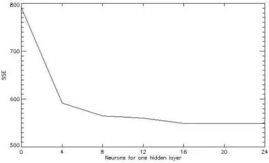
The figure clearly discriminates between the classes. This results from the spectral properties related to the different molecular resonance mechanisms which characterize the surface materials. Using the same data for the sensitivity analysis we were able to generate a training-set with a statistically significant number of pixels for each of the four categories. Previous studies have shown that the training set, notably in terms of its size and compositions, can have a marked impact of the classification accuracy (Foody et al. (1995)). The training datasets were generated considering about 24, 400 pixels. The design of the network put particular emphasis on the selection of the number of hidden units to be considered in the net. To this purpose the plot in Fig. 3.3 was produced, where the SSE value over a test set of more than 1, 000 patterns is reported that corresponds to different numbers of hidden units. It can be seen that, if we consider both the SSE error and the network complexity, the best results were obtained with a 4 − 20 − 20 − 4 topology. Indeed, the increase of the

(36)

Figure 3.2 -Spectral analysis from Quickbird image QB1 for the classes buildings (dashed line), asphalted surface (solid line), bare soil (dash-dotted line), vegetated areas (dotted line).

(37)

number of hidden units did not significantly change the SSE error.

A similar plot is reported in Fig. 3.4 where now a single hidden layer is considered. Again the best result are obtained with around 20 neurons in the hidden layer, however this topology is slightly worse if compared with the two-hidden layer topology. This indicates that the second layer is able to extract additional information from what is already discriminated by the first one. The topology 4 − 20 − 20 − 4 was then finally selected and used to classify the entire image (3, 506, 832 pixels).

Figure 3.3 -SSE values calculated over the test set changing the number of hidden neurons in a two hidden layers topology. The number of units is the same in both layers.

Fig. 3.5 shows the classification map derived using this procedure. The classification accuracy has been assessed by visual comparison with the original high resolution image and by direct inspections on site. We stress the fact that our working area is located at the Tor Vergata University campus, that is almost at the centre of image QB1, allowing direct inspection on site. A ground truth map, corresponding to a subset of the image, has been manually interpreted. We observed that the classification provided by the network is accurate due

(38)

Figure 3.4 -SSE values calculated over the test set changing the number of hidden neurons in a one hidden layer topology.

Figure 3.5 -Classification map of the image QB1 using the optimized topology. Red: bare soil, blue: asphalted surface, white: buildings, green: vegetated areas.

(39)

to its high-level of resolution and we reached a 93% accuracy in the subimage considered.

The whole confusion matrix is reported in 3.1.

Classified as

True

Vegetated Areas Asphalt Building Bare Soil

Vegetated Areas 14864 33 750 2207

Asphalt 132 44785 68 27

Building 1225 29 12634 783

Bare Soil 230 2 512 3229

Table 3.1 - Confusion matrix obtained for image QB1 with the 4 − 20 − 20 − 4 topology. Overall number of pixels: 81510. Overall Error: 5998 pixels (7.36%).

Once the network topology for this kind of problem has been optimized and the performance assessed, we move to investigate the capability of a unique network to provide the classification of different images rather than of a single one. To underline the complexity of this new problem we tested the designed network, developed from the QB1 image, on another QB image. The choice of this new image should follow some similarity criteria with respect to the already classified one. For example it would not be very meaningful to consider a new image characterized by very different land cover classes, such as water, which does not appear in the QB1 image (hence not integrated at all by the network during its training process). Failure of the neural network in this case can be taken for granted and this test would not provide an evaluation of the network generalization capability. Therefore, we decided to choose as a test image a QB image quite similar to QB1. Indeed, the new QB image (QB2) is taken of the same area as the first one, but in a different season and at a slightly different incident angle. In 3.2 we summarize the basic information of the two images analyzed so far and of those that will be considered in the following. If

(40)

the trained network fails in its application to this image it will be unlikely to succeed with many other QB images.

Code Acquisition Date Dimension Off Nadir Location

(pixels) Angle

QB1 03/13/2003 2415 ∗ 1650 8 Degrees Rome, SE outskirts

QB2 05/29/2002 2352 ∗ 1491 11 Degrees Rome, SE outskirts

QB3 07/19/2004 2415 ∗ 1650 23 Degrees Rome, NE outskirts

QB4 07/19/2004 2415 ∗ 1450 23 Degrees Rome city

QB3 07/22/2005 2223 ∗ 1450 12 Degrees Nettuno town

Table 3.2 - Characteristics of the Quickbird images used in the work. All the acquisition times are between 10 : 00 − 10 : 30 a.m.

Figure 3.6 - Automatic classification map from the image QB2 with a net trained with examples taken from image QB1. Red: bare soil, blue: asphalted surface, white: buildings,

green: vegetated areas.

(41)

using the net trained on patterns retrieved from image QB1. For the sake of completeness and for a better interpretation of the results we also produced the classification, reported in Fig. 3.7, that would be obtained applying to the image QB2 the single image classification method developed for image QB1 (a network (4 − 20 − 20 − 4), trained with examples from QB1). The classifica-tion map shown in Fig. 3.7 seems, as expected, rather accurate. Indeed the misclassification percentage computed over the same image subset considered for QB1 is 95% similar to the one obtained in the former case. The classifi-cation result shown in Fig. 3.6 is completely different. Although the network recognizes many patterns and assigns the correct class to the corresponding pixels, entire objects are misclassified, the bare soil class and the built areas class are definitely overestimated and the general noise level produced by the classification is significantly increased. From a quantitative point of view the misclassification rate computed over the subset test image is 56%. Fig. 3.8

Figure 3.7 -Classification map from the image QB2 using a network trained with examples taken from image QB1. Red: bare soil, blue: asphalted surface, white: buildings, green:

(42)

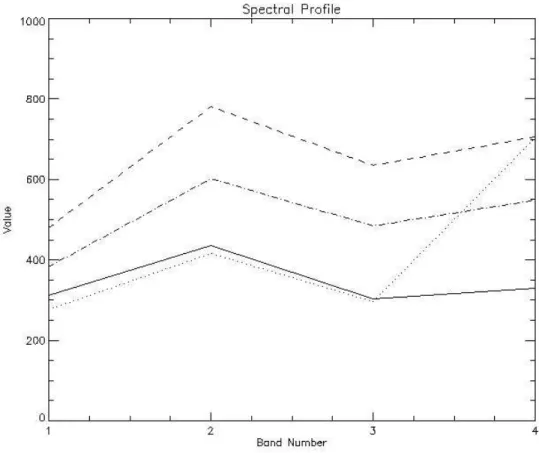
contributes to understanding the classification performance. We observe that even if the shapes of the signatures resemble those plotted in Fig. 3.2, where we can still discriminate between classes, the ranges of the digital number values are significantly different, generating confusion when the network generates its classification response. Thus, the classification of the QB2 image obtained us-ing a network trained on another image, even if taken on the same scenario, is not adequate. This means that to design a network able to provide good clas-sification accuracy for images not used in the training phase is an ambitious goal, even if the classification is performed for a limited number of classes.

Figure 3.8 -Spectral analysis from image QB2 for the training set classes: buildings (dashed line), asphalted surface (solid line), bare soil (dash-dotted line), vegetated areas (dotted line).

(43)

Chapter 4 Methods to “globally”

characterize a (large) urban

area

4.1 The Discrete Fourier Transform

4.1.1 The Discrete Spectrum

Consider now the problem of finding the spectrum (i.e. of computing the Fourier transform) of a sequence of samples. This is the first stage in our com-putation of the Fourier transform of an image. Indeed, the sequence of samples to be considered here could be looked at as a single line of pixels in a digital image. Here we made the assumption that the spectrum of a set of samples is itself a continuous function of spatial wavenumber (ν). For digital processing clearly it is necessary that the spectrum itself also be represented by a set of values, that would, for example, exist in computer memory. Therefore we have to introduce a suitable sampling function in the wavenumber domain. For this purpose consider an infinite periodic sequence of impulses in the wavenumber domain spaced by ∆ν. It can be shown that the inverse transform of this

(44)

4. Methods to “globally” characterize a (large) urban area 44

quence is another sequence of impulses in the spatial domain, spaced ∆ν apart. In this case we are going from the wavenumber domain to the spatial domain rather than vice versa.

4.1.2 Discrete Fourier Transform Formulae

Let the sequence φ(k), k = 0, ..., K be the set of K samples taken of f (x) over the sampling period 0 to x0. The samples correspond to distance kX. Let

the sequence F(r), r = 0, ..., K − 1 be the set of samples of the wavenumber spectrum. These can be derived from φ(k) by suitably modifying the Fourier transform:

X(κ) = Z ∞

−∞

f (x)e−jωxdx (4.1)

In fact, the integral over time can be replaced by the sum over k=0 to K-1, with dx replaced by ∆x, the sampling increment. The continuous function f(x) is replaced by the samples φ(k) and κ = 2πf is replaced by 2πr∆ν with r = 0, ..., K − 1. Thus κ = 2πr/X0. The spatial variable X is replaced by

kX = kX0/K, k = 0, ..., K − 1. With these changes 4.1 can be written in

sampled form as F (r) = X K−1_X k=0 φ(k)Wrk, r = 0, ..., K − 1 (4.2) with W = e−j2π/K. (4.3)

Equation 4.2 is known as the discrete Fourier transform (DFT). In a similar manner a discrete inverse Fourier transform (DIFT) can be derived that allows reconstruction of the spatial sequence φ(k) from the wavenumber samples F(r). This is

(45)

φ(k) = X0 K−1_X

r=0

F (r)Wrk, k = 0, ..., K − 1 (4.4) Sobstitution of 4.1 into 4.4 shows that those two expressions form a Fourier transform pair. This achieved by putting k=l in 4.4 so that

φ(l) = 1 X0 K−1_X r=0 F (r)W−rl= 1 X0 K−1_X r=0 ·X K−1_X k=0 φ(k)Wr(k−l) = 1 K K−1_X k=0 φ(k)· K−1_X k=0 Wr(k−l) (4.5) The second sum in this expression is zero for k 6= l; when k = l is K, so that the right hand sid of the equality then becomes φ(l) as required. An interesting aspect of this development has been that X has cancelled out, leaving 1/K as the net constant from the forward and inverse transforms. As a result 4.2 and 4.4 could conveniently be written

F (r) = K−1_X k=0 φ(k)Wrk r = 0, ..., K − 1 (4.6) φ(k) = 1 K K−1_X r=0 F (r)W−rk k = 0, ..., K − 1 (4.7)

4.1.3 Properties of the Discrete Fourier Transform

Three properties of the discrete Fourier transform and its inverse are of importance here:

• Linearity: Both the DFT and DITF are linear operations. Thus if F1(r)

is the DFT of φ1(k) and F2(r) is the DFT of φ2(k) then for any complex

constants a and b, aF1(r) + bF2(r) is the DFT of aφ1(k) + bφ2(k).

• Periodicity: from 4.3, WK = 1 and WkK = 1 for k integral. Thus for r0_{= r + K}

(46)

4. Methods to “globally” characterize a (large) urban area 46 F (r0) = X K−1_X k=0 φ(k)W(r+K)k = F (r) (4.8) Thus in general F (r + mK) = F (r) (4.9) φ(k + mK) = φ(k) (4.10)

where lm is an integer. Thus both the sequence of spatial samples and the sequence of wavenumber samples are periodic with period K. This is consistent with the development of Sect. 4.1.1 and has two important implications. First, to generate the Fourier series components of a pe-riodic function, samples need only be taken over one period. Secondly, sampling converts an aperiodic sequence into a periodic one, the period being determined by the sampling duration.

• Symmetry: Let r0 _{= K − r in 4.1, to give}

F (r0) = X

K−1_X k=0

φ(k)W−rkWkK (4.11)

Since WkK _{= 1 this shows F (K −r) = F (r)}∗ _{where ∗ represents the}

com-plex conjugate. This implies that the amplitude spectrum is symmetric about K/2 and the phase spectrum is antisymmetric (i.e. odd).

4.2 The Discrete Fourier Transform of an Image

4.2.1 Definition

In the foregoing section we have treated functions with a single independent variable. That variable could have been the position along a line of an image.

(47)

Now functions with two independent variables will be examined. Let

φ(i, j), i, j = 0, ..., K (4.12)

be the brightness of a pixel at location i, j in an image of KxK pixels. The Fourier transform of the image, in discret form, is described by

Φ(r, s) = K−1_X i=0 K−1_X j=0 φ(i, j)exp[−j2π(ir + js)/K] (4.13) An image can be reconstructed from its transform according to

Φ(r, s) = 1 K2 K−1_X i=0 K−1_X j=0 φ(i, j)exp[+j2π(ir + js)/K] (4.14)

4.2.2 Evaluation of the Two Dimensional, Discrete Fourier Trans-form

Equation 4.13 can be written as

Φ(r, s) = K−1_X i=0 Wir K−1_X j=0 φ(i, j)Wjs (4.15)

with W = e−j2π/K as before. The term involving the right hand sum can be recognised as the one dimensional discrete Fourier transform

Φ(i, s) =

K−1_X j=0

φ(i, j)Wjsi = 0, ..., K − 1 (4.16) In fact it is the one dimensional transform of the ith row of pixels in the image. The result of this operation is that the rows of an image are replaced by their Fourier transforms; the transformed pixels are then addressed by their wavenumber index s across a row rather the positional index j. Using 4.16 in 4.15 gives