UNIVERSITY
OF TRENTO
DEPARTMENT OF INFORMATION AND COMMUNICATION TECHNOLOGY
38050 Povo – Trento (Italy), Via Sommarive 14
http://www.dit.unitn.it
IMAGE FUSION TECHNIQUES FOR REMOTE SENSING
APPLICATIONS
G.Simone, A.Farina, F.C.Morabito, S.B.Serpico and L.Bruzzone
2002
Technical Report # DIT-02-0025
IMAGE FUSION TECHNIQUES FOR REMOTE SENSING
APPLICATIONS
AUTHORS:
G.Simone
1, A.Farina
2, F.C.Morabito
1, S.B.Serpico
3, L.Bruzzone
41
NeuroLab – DIMET - University “Mediterranea” of Reggio Calabria
2
Alenia Marconi Systems, S.p.A.
3Dept. of Biophysical and Electronic Engineering – University of Genoa, Italy
4
IMAGE FUSION TECHNIQUES FOR REMOTE SENSING
APPLICATIONS
Abstract
Image fusion refers to the acquisition, processing and synergistic combination of information provided by various
sensors or by the same sensor in many measuring contexts. The aim of this survey paper is to describe three typical
applications of data fusion in remote sensing. The first study case considers the problem of the Synthetic Aperture
Radar (SAR) Interferometry, where a pair of antennas are used to obtain an elevation map of the observed scene; the
second one refers to the fusion of multisensor and multitemporal (Landsat Thematic Mapper and SAR) images of the
same site acquired at different times, by using neural networks; the third one presents a processor to fuse
multifrequency, multipolarization and mutiresolution SAR images, based on wavelet transform and multiscale Kalman
filter. Each study case presents also results achieved by the proposed techniques applied to real data.
Keywords.- Remote Sensing, Synthetic Aperture Radar (SAR), SAR Interferometry, Neural Networks, Discrete Wavelet Transform (DWT), Multiscale Kalman Filter
1. Introduction
Remote sensing [1] is a science with applications ranging from civilian to surveillance and military. Remote sensing systems measure and record data about a scene. Such systems have proven to be powerful tools for the monitoring of the Earth surface and atmosphere at a global, regional, and even local scale, by providing important coverage, mapping and classification of land cover features, such as vegetation, soil, water and forests. The degree of accuracy achieved in classification depends on the quality of the images, on the degree of knowledge possessed by the researcher, and on the nature of the cover types in the area. For instance, correlations can then be drawn among drainage, superficial deposits and topographic features, in order to show the relationships that occur between forest, vegetation and soils. This provides important information for land classification and land-use management. The sensors that acquire the images, are typically classified as airborne or space borne sensors, if they are placed, respectively, on an airplane or a satellite; furthermore, they can acquire information in different spectral bands on the basis of the exploited frequency, or at different resolutions. Therefore, a wide spectrum of data can be available for the same observed site. For many applications the information provided by individual sensors is incomplete, inconsistent, or imprecise [2,3,4]. Additional
sources may provide complementary data, and fusion of different information can produce a better understanding of the observed site, by decreasing the uncertainty related to the single sources [5,6,7]. Images may be provided by radars and by heterogeneous sensors. For instance, multitemporal radar images [1,8,9] of the same scene are needed to detect changes that occur in the considered scene between two or more observations; multidimensional images, provided by radar and non radar sensors, facilitate the classification of scene segments because multispectral and multipolarization data increase the separation between the segments. In the interpretation of a scene, contextual information is important: in an image labeling problem, a pixel considered in isolation may provide incomplete information about the desired characteristics. Context can be defined in the frequency, space and time domains. The spectral dimension refers to different bands of the electro-magnetic spectrum. These bands may be acquired by a single multispectral sensor, or by more sensors operating at different frequencies. The spectral context improves the separation between various ground cover classes compared to a single -band image [1]. Furthermore, since the electromagnetic incident/backscattered wave depends also on the polarization, then the properties of the examined area can be studied by varying the polarization of the incident/backscattered wave. Therefore, complementary information about the same observed scene can be available in the following cases:
− data recorded by different sensors (multisensor image fusion);
− data recorded by the same sensor scanning the same scene at different dates (multitemporal image fusion);
− data recorded by the same sensor operating in different spectral bands (multifrequency image fusion);
− data recorded by the same sensor at different polarizations (multipolarization image fusion);
− data recorded by the same sensor located on platforms flying at different heights (multiresolution image fusion).
In this paper, three different fusion applications in remote sensing are presented:
• the Synthetic Aperture Radar (SAR) interferometry [1,8,9,10] is proposed as a data fusion method that, by exploiting the data recorded by two different antennas about the same scene, allows one to obtain an elevation map of the area;
• multitemporal and multisensor experiments [11,12] are presented to describe a system that integrates information from different sensors (SAR and LANDSAT) acquired at different dates, by using neural networks;
• multifrequency, multipolarization and multiresolution fusion [13-15] is described for data acquired by SAR sensors in different measuring contexts , based on the discrete wavelet transform (DWT) and multiscale Kalman filter (MKF).
The paper is organized into 5 Sections. Section 2 describes the SAR interferometry study case; the multisensor and multitemporal image fusion is presented in Section 3; Section 4 describes a multipolarization, multifrequency and multiresolution image fusion example, taking into account also the radiometric correction and spatial registration of the images. Conclusions are drawn in Section 5.
2. The SAR Interferometry
A Synthetic Aperture Radar (SAR) [1,8] is an active coherent imaging system that, combining the signals received by a moving radar antenna operating in the microwave region of the spectrum, estimates the relative reflectivity of a spatial distribution of scatterers. The resulting imagery has various possible uses such as in surveillance, oceanography, military applications and agriculture, since the obtained images have a high resolution, independent of the weather conditions. Furthermore, SAR data are used not only for monitoring applications, but also to obtain elevation maps of the observed scene [9,10]. A SAR gives an image of the phase and amplitude of the reflected radiation as a function of the azimuth and slant range coordinates, that is, of the coordinates parallel and perpendicular to the trajectory of the antenna. Observing a given scene from two SAR antennas with distinct trajectories (not necessarily at the same time) allows to perform a triangulation and, in principle, to determine the three-dimensional position of the scattering points, that is, the elevation map of the observed scene. If the two SAR images are co-registered, i.e.: if the corresponding pixels of the two SAR images pertain to the same points of the observed scene, the phase difference of the signals measured in the corresponding pixel of the two images is a very sensitive measure of the length difference of the paths traveled by the signals. From this difference and from the knowledge of the distance of the observed points from one of the SAR trajectories, the 3D position of the points is immediately calculated. Unfortunately, SAR interferometry fails when the scenes imaged by the two SAR systems are not really the same scene, due to a too large distance between the trajectories of the two SAR antennas, or to a too large time elapsed between the two surveys. In these cases, the two images may not be sufficiently correlated: the phase difference in the corresponding pixel of the two images is not useful to determine the distance difference of the scene from the SAR systems, and there is not coherence. Other limitations are given by the occurrence of layover and shadow phenomena. Layover takes place when more than one point of the observed scene is at the same distance from the trajectory of the SAR system; in this case, the signal in the pixel of the SAR image is an average of the signals corresponding to the different points. Shadow occurs when a point of the observed scene is not seen fro m the radar system because it is covered by other points; that point does not contribute to the measured signal.
2.1. Wrapped and Unwrapped Phases
Each of the two SAR images gives only a measure of the phase of the received electromagnetic radiation modulo 2 . π The phase difference modulo 2 can be calculated from the two images, while it is necessary to determine the whole π phase difference of the signals in the two images to determine the 3D position of the corresponding points in the scene. Therefore, it is important to unwrap the available phase difference, that is, to reconstruct the available phase difference in the corresponding pixel of the two images from the knowledge of that difference modulo 2 . These two quantities π are referred to as unwrapped and wrapped interferometric phases, respectively. In interefometric studies, high resolution images are processed; it can be supposed that the height difference between neighboring pixels is sma ll: this assumption fails when the topography changes very rapidly in a restricted area. For this reason, all methods assume that the unwrapped interferometric phase in neighboring pixels differ by a quantity that is almost always less than π in absolute value. This hypothesis is used to estimate from the wrapped interferometric phase the neighboring pixel differences, that is, the discrete gradient of the unwrapped interferometric phase. The unwrapped interferometric phase is then reconstructed, up to an additive constant, from the estimate of its discrete gradient. The additive constant is determined from a priori information on the scene, that is, the knowledge of the elevation of one point in the scene.
2.2. The Unwrapping Algorithm
The methods proposed differ in the way they overcome the difficulty posed by the fact that the neighboring pixel differences of the unwrapped interferometric phase may not be everywhere less than π . This can be due to noise, or to the fact that the observed scene becomes too steep, that is, nearly perpendicular to the view direction. Further challenges are posed by the occurrence of layover, shadow, or lack of coherence phenomena. The phase unwrapping algorithm in [10] is based on the projection of a discrete vector field onto the linear subspace defined by the “irrotational property” of a discrete gradient vector field. A vector field is called irrotational when the curl of this vector field is 0. The projection onto the linear subspace characterized by the “irrotational property” of a discrete gradient vector field is a local operation in the Fourier space. Therefore, only O
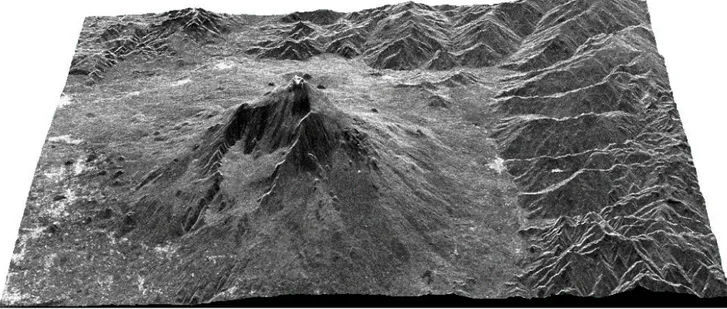
(
NlogN)
elementary operations are required to project discrete vector field of N pixel, which is the computational complexity of the fast Fourier transform. Based on the proposed projection algorithm, the phase unwrapping can be obtained by projecting the estimated discrete gradient field onto the “irrotational” subspace and then “integrating” the resulting discrete gradient vector field. The points belonging to steep and layover regions are isolated by means of further information: a simple correction is performed on the estimate of the discrete gradient of the unwrapped interferometric phase, to reduce the systematic errors in the estimated unwrapped phase gradient. For greater details on the exploited algorithm, the reader is referred to [10]. The proposed phaseunwrapping algorithm is tested on a pair of ERS-1 and ERS-2 SAR images of the Etna’s volcano (Fig.1), acquired on September 1995. The elevation obtained is in qualitative agreement with the elevation reported in geographic maps.
Fig. 1.- Reconstructed elevation of the Etna’s volcano (courtesy of Dr. M. Costantini).
3. Fusion of Multitemporal-Multisensor Remotely Sensed Images
In several applications, the capability of SAR sensors to acquire images during day and night and with all weather conditions has proved to be precious. However, depending on the kinds of terrain cover types, the information provided by the SAR data alone may be not sufficient for a detailed analysis. A possible solution to this problem may derive from the integration of SAR data with optical data (or multisensor data) of the same site acquired at a different time [11,12,16,17]. Several methodologies have been proposed, in the scientific literature, for the purpose of multisensor fusion; they are mainly based on statistical, symbolic (evidential reasoning), and neural-network approaches. Among statistical methods, the “stacked-vector” approach is the simplest one [18]: each pixel is represented by a vector that contains components from different sources. This approach is not suitable when a common distribution model cannot describe the various sources considered. The Dempster-Shafer evidence theory [19] has been applied to classify multisource data by taking into account the uncertainties related to the different data sources involved [20,21,22]. Neural-network classifiers [11,12] provide an effective integration of different types of data. The non-parametric approach they implement allows the aggregation of different data sources into a stacked vector without need for assuming a specific probabilistic distribution of the data to be fused. Results, obtained by using different kinds of multisource data, point out the effectiveness of neural network approaches for the classification of multisource data. Concerning the classification process in a multitemporal environment, only a few papers can be found in the
remote-sensing literature. Cascade classifiers [23] based on the generalization of the Bayes optimal strategy to the case of multiple observations have been proposed: multitemporal information has been used assuming that the behavior of these processes can be modeled by a first-order Markov model. Methods based on contextual classification that accounts for both spatial and temporal correlations of data, have been developed [24]: the feature vectors are modeled as resulting from a class-dependent process plus a contami nating noise process; the noise process is considered autocorrelated in both space and time domains.
3.1. The “Compound” Classification
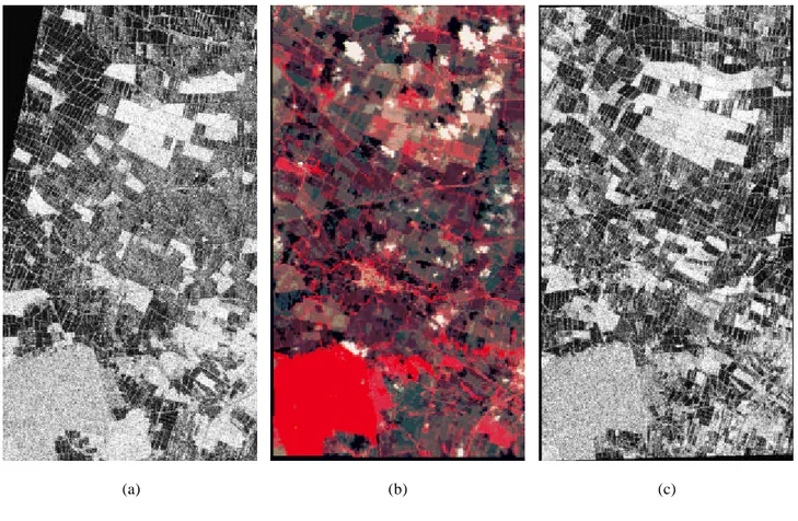
The experiment summarized in this section has been presented in [12], to which the reader is referred for further information. A multitemporal and multisensor data set (Fig.2) has been considered for this experiment, referring to an
(a) (b) (c)
Fig. 2.- Multitemporal and Multisensor data set consisting of: (a) SAR image (April 1994);
(b) optical image (May 1994); (c) SAR image (May 1994). (from [12])
agricultural area in the basin of the Po River, in northern Italy. Such a data set consists of an image acquired by the ERS-1 SAR sensor in April 1994 and a pair of images acquired in May 1994 by the Landsat TM and the ERS-1 SAR sensors. These two latter images have been registered to the ERS-1 SAR April image. The LANDSAT Thematic Mapper (TM) is an advanced optical sensor (multispectral scanner) designed to achieve high spatial resolution
(30m×30m), sharp spectral separation (images are acquired simultaneously in seven spectral bands, from the wavelength of 0.45µm to 2.35µm), high geometric fidelity, and good radiometric accuracy and resolution. Typically, TM Bands 4, 3, and 2 can be combined to make false-color composite images where band 4 represents red, band 3, green, and band 2, blue. This band combination makes vegetation appear as shades of red, brighter reds indicating more vigorously growing vegetation. Soils with no or sparse vegetation will range from white (sands) to greens or browns depending on moisture and organic matter content. Water bodies will appear blue. Deep, clear water will be dark blue to black in color, while sediment-laden or shallow waters will appear lighter in color. Urban areas will appear blue-gray in color. Clouds and snow will be bright white; they are usually distinguishable from each other by the shadows associated with the clouds.
The approach presented in this section is based on the application of the Bayes rule for minimum error to the “compound” classification [25] of pairs of multisource images acquired at different dates. In particular, two multisource image data sets I and 1 I , acquired at two times 2 t and 1 t , respectively, are analyzed to identify the land-cover classes 2
present in the geographical area to which the data are referred. Each data set may contain images derived from different sources: in our cas e, the SAR and LANDSAT TM sensors. The input images are supposed to be co-registered and transformed into the same spatial resolution; each pair of temporally correlated pixels
(
x1, x2)
, x1∈I1 and x2∈I2, is described by a pair of feature vectors(
X1, X2)
. Let Ω={
ω1,ω2,...,ωM1}
be the set of possible land-cover classes at time1
t , and let Λ=
{
λ1,λ2,...,λM2}
be the set of possible land-cover classes at time t . The “compound” classification of 2each pair of pixels
(
x1, x2)
is aimed at finding the pair of classes (ωm,λn) that have the highest probability to beassociated with them. It is possible to prove that, under the simplifying hypothesis of class-conditional independence in
the time domain, this task can be carried out according to the following rule [12]:
maxωi, λj
{
P(ωi / X1) P(λj / X2 ) P(ωi , λj )/
P(ωi ) P(λj )}
(3.1)The available ground truth can be used to generate two training sets (one for each date) useful to estimate the a priori and the posterior probabilities of classes. In particular, the a priori probabilities P
( )
ω and i P( )
λ are estimated by jcomputing the occurrence frequency of each class in the t1 and t2 training sets, respectively. The posterior probabilities
of classesP
(
ωi | X1)
and P(
λj| X2)
are estimated by applying two multilayer perceptron neural networks, trained with the backpropagation algorithm, to single-date multisource images. The joint probabilities of classesP
(
ω
i,
λ
j)
, which model the temporal correlation between the two multisource images, are estimated by using the EM algorithm [26]. Inparticular, it is possible to prove that the equation to be used at the k+1 iteration for maximizing the likelihood function is the following [12]:
(
)
( )
( )
(
(
)
)
(
)
(
)
( ) ( )
(
) (
)
∑
∑ ∑
⋅ = Ω ∈ ∈Λ + ⋅ ⋅ ⋅ ⋅ ⋅ ⋅ ⋅ ⋅ ⋅ = NM q q m q n m k n k m n k q j q i j i k j i j i k n m X P X P P P P X P X P P P P M N P 1 2 1 2 1 1 | | , | | , 1 , ω λ λ ω λ ω λ ω λ ω λ ω λ ω λ ω (3.2)where N⋅M is the total number of pixels to be classified in each image and Xk q
is the qth pixel of the image I . It is k
worth noting that in the initialisation step equal probabilities are assigned to each pair of classes. The algorithm is iterated until convergence. At convergence, the obtained joint probabilities are used in equation (3.1) together with the estimated a priori and posterior probabilities of classes to derive the land-cover maps.
3.2. Experimental Results
The four dominant land cover types in April for the study area have been considered, namely: wet rice fields, bare soil, cereals and wood. In May, an additional cover type (corn) has been included, increasing the size of the set of possible classes to five. For the May data set, 11 features have been considered: 6 intensity features from the Landsat TM image (corresponding to all bands but the infrared thermal one), 1 intensity feature from the ERS-1 SAR (C band, VV polarization) image and 4 texture features (entropy, difference entropy, correlation and sum variance) computed from the ERS-1 SAR image using the gray-level co-occurrence matrix. For the April image, only the above 5 features (1 intensity and 4 texture features) derived from the ERS-1 SAR image have been utilized. For each date, a feedforward MLP neural network has been trained independently (Fig.3): a MLP to estimate the posterior class probabilities of the pixels of the April image (from single sensor data); a different MLP to estimate the analogous probabilities for the May image (from multisensor data). The number of input and output neurons corresponded, respectively, to the number of features and of classes defined for each date; one hidden layer of eight neurons has been considered in both cases. The EM algorithm has been applied and reached the convergence after six iterations to provide the estimate of the joint class probabilities.
The classification results obtained for the April image independently (without fusion) and with data fusion by the proposed approach are illustrated in Table 1. They are expressed in terms of percent average accuracy (i.e. the mean value of the accuracy over the different classes).
Fig. 3.- Block scheme of the “compound” classification technique. (from [12])
A significant improvement of the average accuracy (i.e. +17%) has been obtained thanks to data fusion, showing that classes which are poorly discriminated by the SAR sensor alone at a given date can be recovered by the use of the multisensor information related to another date. In this case, the improvement is mainly related to the class "cereals", with an increase of accuracy from 16.67% (without fusion) to 75.0% (with fusion). The early growth of this plant in April makes difficult its discrimination with the SAR sensor, only. The multisensor information, extracted from the May image, in which the discrimination of the class "cereals" is much easier (84.26% without temporal fusion), played a valuable role to recover this class.
Area Without Fusion With Fusion
Wet Rice Fields 98.54 99.46
Baresoil 93.11 97.18
Cereals 16.67 75.0
Wood 92.32 97.0
Average Accuracy 75.16 92.16
Table 1.- Accuracy obtained for the test set of the April 1994 image
4. Fusion of Multipolarization-Multifrequency-Multiresolution SAR Images
Data fusion systems have also been developed to fuse information carried by multipolarization, multifrequency and multiresolution data acquired by the same sensor [5,6,27-30]. In the case of active microwave and radio sensors, the data consist of the reflection of the scattering properties of the surface in the microwave region [1,8,31]. A natural surface can be mathematically described as a series of backscatterers, that reflect the wave produced by the sensor. The reflected wave depends on three different aspects related to the local geometry and to the incident wave: incidence angle, polarization and frequency. At small angles, the backscattered return is dependent on the angle of incidence, and it provides information on the surface slopes distribution for topography at a scale significantly larger than the wavelength. At wide angles, the return signal provides information about the small-scale structure. Thus, when images, acquired by the same sensor at different incidence angles, are fused, since the received backscattered radiation is strongly depending on the angle and, thus, on the topography, it is necessary to apply radiometric corrections. This can be done by using a digital elevation model (DEM); a correction of the considered images can be exploited to obtain a real view of the observed scene [9,32,33].The backscatter cross section of natural surfaces also depends on the polarization of the incident wave; four different modes are usually considered: HH, horizontally polarized emitted, horizontally polarized received and similarly for HV, VV and VH. It is possible to show that the same scene has a different behavior at different polarizations: therefore, when data at different polarizations about the same scene are available, the information content about the observed region can be increased by fusing the multipolarization information. The same observation can be addressed for multifrequency data; particularly in this case, the operating frequency is a key factor in the penetration depth [1]: an L-band (20 cm wavelength) signal will penetrate about 10 times deeper than a Ku band (2 cm wavelength) signal thus providing access to a significant volumetric layer near the surface. In addition, the behavior of the backscatterer, as a function of frequency, changes on the basis of the surface types. Therefore, if the images acquired in many regions of the spectrum are fused, the output image will carry useful information about specific backscatterers otherwise visible just in single frequencies. More specifically, when a SAR sensor scans a scene, typically, data at many polarizations and at many frequencies are available; furthermore, the same scene can be observed by SAR sensors that are located on flying platforms at different heights, and therefore, data at different resolutions are available.
4.1. Radiometric Correction
An important operation to be accomplished, before fusing the images, is the radiometric correction: this step is used to reduce the effects of the acquisition context on the recorded data; these effects are particularly evident in the case of
microwave and radio frequency sensors, where the topography of the scene significantly changes the reflection properties of the backscatterers [9,32,33]. Previous studies have shown that for SAR imagery from non flat terrain, the topography must be taken into account in the radiometric correction for pixel scattering area. In the SAR image, the pixel represents the intensity of the electromagnetic wave scattered by the observed surface: therefore, it is necessary to take into account the action of the topography on this scattered signal received by the antenna. In other words, it is important to compute for each pixel a normalization factor, depending on the slant-range pixel spacing in the range direction δ , on the slant-range pixel spacing in the azimuth direction r δ , and on the local radar incidence angle in the a range direction η (Fig.4). r
Fig. 4.- Imaging geometry in the range direction. (from [32])
The radiometric correction consists of the computation of this normalization factor, that, in its expression, contains the correction of the changes in the pixel intensity due to changes in the topography. The SAR image is acquired in a plane where the two axes are called azimuth and range: the azimuth direction is the line parallel to the flight line; the range direction is the line perpendicular to the flight line. The δ factor is the distance in the range direction between two r points on the surface which can still be separable; the δ factor corresponds to the two nearest separable points along a an azimuth line. It is possible to show that this normalization factor is [32,33]:
( )
r a r A η δ δ sin ⋅ = (4.1)To compute this normalization factor A, the DEM of the area, that is a topographic representation of the observed scene, and the flight path of the platform on which the radar is located, are needed. Each pixel of the input SAR image is multiplied by the factor A: this operation corresponds to the normalization of the backscattering area, and, therefore, to the correction of the intensity of each pixel. Fig.4 describes the problem geometry in the range plane: the parameters depicted in the Figure are the ones used in the algorithm to compute the normalization factor, and it gives an explanation of the physical meaning of the symbols δ , r δ and a η , above described. This algorithm, implemented in r Matlab® code, has been used to radiometrically correct the input data, and to obtain a real view of the scene.
4.2. DWT and Salience Computation for Multifrequency-Multipolarization Image Fusion
The next step is the fusion of the multipolarization and multifrequency images, that have been radiometrically corrected. Simple procedures to perform image fusion are the IHS method [34] and the method of principal components analysis (PCA) [27]. In the case of PCA, each pixel in the fused image is the weighted sum of the pixels in the input images, by using as weights the eigenvectors corresponding to the maximum eigenvalue of the covariance matrix. If there is a low correlation between the detailed surface structures in the input images to be fused, the PCA method does not preserve the fine details (similar problems arise also with the IHS method). Therefore, techniques that integrate the fine details of the input data in the fused image are preferred. This is the reason for which pyramidal methods are popular [15,28-30,35-38]: a pyramid is firstly constructed transforming each source image into the pyramid domain; then a fused pyramid is constructed, selecting the coefficients from the single pyramids, and the matched image is computed by an inverse pyramid transform. The manner in which the pyramid domain is constructed changes on the basis of the applied technique: when we fix the method to decompose the data, the pyramid domain consists of the decomposed data, that is, of the coefficients provided by the decomposing technique; since the decomposition coefficients represent the input data at different resolutions, and since the size of the data decreases at higher resolution, the structure of the transformed data can be represented by a pyramid. We are interested in the information carried by the full resolution data in the spatial domain: therefore, after the fusion step in the pyramid domain, it is necessary to transform the fused data in the original domain; this is accomplished by using an inverse transformation, based on the technique applied to transform data into the pyramid domain. The pyramid-based fusion techniques typically differ in the pyramid construction method, and in the technique used to select the coefficients from the images to be fused. Popular methods are based on laplacian and gradient pyramids [28], where the gradient technique guarantees improved
stability and noise immunity; recently, the wavelet transform has been shown as a powerful method to preserve the spectral characteristics of the multipolarization and multifrequency images [15], allowing decomposition of each image into channels based on their local frequency content. After the construction of the input pyramids, the coefficients can be fused on the basis of specific pattern selective techniques: an information measure extracts the information from the input pyramids, and the match measure is used to fuse the extracted information. The simplest methods are based on the selection of the higher value coefficients; other methods are based on salience computation [28], that estimates the evidence of a pattern related to the information contained in the neighboring area. The technique, exploited throughout this paper, is based on the use of a pyramidal method that uses the discrete wavelet transform (DWT) [39,40]: it consists of a decomposition of an image in sub-images, that represent the frequency contents of the original image at different levels of resolution. Due to desirable properties concerning approximation quality, redundancy and numerical stability, the low pass and high pass filters, used to compute the sub-images, have been constructed on the basis of the Daubechies wavelet family. The images acquired by the same sensor at different frequencies or polarizations have been fused, by computing the wavelet pyramid and by linearly combining the wavelet coefficients. In order to acquire the information carried by each pyramid, the salience of each pattern has been considered [28]: it can be defined as the local energy of the incoming pattern within neighborhood p
(
)
=∑
( ) (
+ +)
' ,' 2 , , ' , ' ' , ' , , , j i l k i j i i j i l k j i p D S (4.2) where:− S is the salience measure,
− p is a window function with unitary value when 1≤i'≤r and 1≤ j'≤q, and zero value elsewhere; this function is used as a local window on the wavelet pyramid around the considered pixel (i,j); in the presented experiment, the value of parameters r and q is 5; this value has been fixed by using a trial and error technique, and they are related to the level of detail in the images being considered;
− D is the pyramid, and
(
i,j,k,l)
are the row and column sample position, level and orientation indexes inside the pyramid structure. When the salience of the coefficient( )
i,j with level k and orientation l is computed, the local window allows us to acquire the neighboring coefficients present in a window r×qpixels around the considered point.The salience of a particular component pattern is high if that pattern plays a role in representing important information in a scene; it is low if the pattern represents unimportant information, or if it represents corrupted image data.
After this salience computation step, applied to the single pyramids A and B, of two images to be fused, a match measure has to be computed to combine the information carried by each pyramid; this match measure is defined on the basis of the salience measure, as the following [28]:
(
)
( ) (
(
) (
) (
)
)
l k j i l k j i l k j j i i l k j j i i j i l k j i B A j i B A AB , , , , , , , , ' , ' , , ' , ' ' , ' 2 , , , ,'' S S D D p M ⋅ + + ⋅ + + ⋅ ⋅ =∑
(4.3)The combined pyramid can be computed by using the following expression:
(
i j k l)
A(
i j k l)
A(
i j k l)
B(
i j k l)
B(
i j k l)
C , , , w , , , D , , , w , , , D , , ,
D = ⋅ + ⋅ (4.4)
and
If MAB
(
i,j,k,l)
≤α⇒wMIN =0 and wMAX =1 (4.5) if MAB(
i,j,k,l)
>α⇒ − − − = α 1 1 2 1 2 1 AB MINw M and wMAX =1−wMIN (4.6)
if SA
(
i,j,k,l)
≥SB(
i,j,k,l)
⇒wA(
i,j,k,l)
=wMAX and wB(
i,j,k,l)
=wMIN (4.7) else if SA(
i,j,k,l)
<SB(
i,j,k,l)
⇒wA(
i,j,k,l)
=wMIN and wB(
i,j,k,l)
=wMAX (4.8)where α is a threshold fixed by the Operator. The final step is to use the inverse discrete wavelet transform to obtain the fused image.
The data used in this Section consist of airborne and space borne images acquired over the San Francisco Bay area, courtesy of JPL, (Jet Propulsion Laboratory, CA, USA), (Figs.5-8). The polarimetric (POLSAR) dataset has been acquired in L-, C- and P- bands with the bandwidths 40.00 MHz and 20.00 MHz (CM5599 and CM5598 images) with different spatial resolution (6.662 m along range and 18.518 m along azimuth for the CM5599 image; 13.324 m along range and 18.518 m along azimuth for the CM5598 image). The interferometry dataset has been acquired in L- and C- bands, with a spatial resolution of 10 m along range and 10 m along azimuth (TS0711). These first two datasets have been acquired during the JPL-AIRSAR Mission. The space borne image has been acquired during the SIR-C/X-SAR Mission, in L- and C- bands, with the HH and HV polarizations, with a spatial resolution of 25 m along range and 25 m along azimuth.
Fig.5.- JPL-AIRSAR POLSAR CM5598 C-band image. Fig.6.- JPL-AIRSAR POLSAR CM5599 C-band image.
Fig.7.- JPL-AIRSAR POLSAR TS0711 C-band image. Fig.8.- SIR-C/X-SAR C-band HV-polarization image.
4.3. Spatial Registration
The images, output of the multifrequency and multipolarization fusion process, will be the input of the multiresolution fusion process. Since they are acquired in different geometries, they have to be co-registered to refer the data to a commo n regular grid; in this way, each pixel of each image will correspond to the homologous pixels of the remaining images [9]. For this reason, an automatic technique has been implemented in Matlab® code, and it matches two images to a common grid. We have chosen the CM5599 image as reference image, and we have matched the other images (CM5598, TS0711 and SIR-C) to the CM5599 image. The algorithm consists of the following steps:
− three points, that are homologous, identical or corresponding image points, have to be manually identified in the two images;
− to improve the registration performance, the technique can be iterated by using as reference points more than three points.
Resampling operations are necessary when one of the two images has a “small” size with respect to the second one: in this case, when the “small” image has to be co-registered to the “large” image, new pixels have to be added to the “small” image; in our experiments, the value of the added pixels has been computed by interpolating the values of the neighboring pixels. Obviously, the information carried by the added pixels has not any radiometric fidelity, since the values reflect the radiometric information carried by the neighboring pixels: if the scene has not strong variations in the topography, then the added values can be considered a good approximation of the real changes in the radiometric information of the considered area. This algorithm has been used to obtain images that have the same size: these data will be processed by the following multiresolution fusion step.
4.4. MKF Algorithm for Multiresolution Image Fusion
After the spatial registration, the images are ready for the mu ltiresolution fusion process. Also in this case the pyramidal techniques can be utilized; other methods, recently proposed, consist of the use of scale -recursive models, based on multilevel trees (Fig.9). The key of this multiple scale filtering is to consider the scale as an independent variable as the time, such that the description at a particular scale captures the features of the process up to that scales that are relevant for the prediction of finer scale features; this algorithm is considered as an extension of the Kalman filter to the scale variable, and it is known as multiscale Kalman filtering [29,35-38]. An image can be decomposed from the coarse to the fine resolution: at the coarsest resolution, the signal will consist of a single value. At the next resolution, there are q=4
values, and, in general, at the mth resolution, we obtain qm values. The values of the multiscale representation can be described by the index set
(
m ,,i j)
, where m represents the resolution and( )
i,j the location index. To describe the model, an abstract index λ is used to specify the nodes on the decomposition tree; γλ specifies the parent node of λ. The multiscale Kalman filtering technique is used to obtain optimal estimates of the state X( )
λ described by the multiple scale model using observations Y( )
λ at a hierarchy of scales. This scheme proceeds in two steps: downward and upward [32-35]. The multiple scale downward (coarse-to-fine resolution) model is given by:( ) ( ) ( ) ( ) ( )
λ Aλ Xγλ Bλ WλX = ⋅ + ⋅ (4.9)
( ) ( ) ( ) ( )
λ Cλ Xλ VλSince X
( )
γλ represents the state at a resolution coars er than X( )
λ , A( ) ( )
λ X⋅ γλ can be considered as a prediction term for the finer level; B( ) ( )
λ W⋅ λ is the new knowledge that we add from one scale to the next. The noisy measurements( )
λY of the state X
( )
λ , the measurement Equation (4.10), combined with the Equation (4.9), form the state estimation problem. The covariance matrices of the state and of the measurements are computed by the following equations:( )
λ [( )
λ T( )
λ]X EX X
P ≡ ⋅ (4.11)
Corresponding to the above downward model, the upward (fine-to-coarse resolution) model is:
( ) ( ) ( )
γλ Fλ Xλ W( )
λ X = ⋅ + (4.12) where( )
λ =( )
γλ ⋅( )
λ ⋅ −1( )
λ X T X A P P F (4.13)4.5. Experimental Results
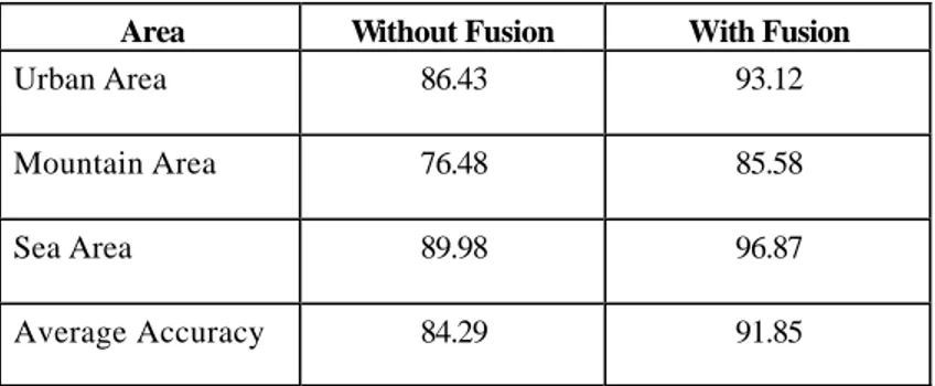
To evaluate the system performance, and to evaluate how the information flows from the input images to the output images, two different tests have been carried out on the considered datasets: a classification test and a straight line detection test, as in typical Automatic Target Recognition (ATR) applications in remote sensing. The classification test has been carried out by using a least square classifier. Three different areas have been considered to be present on the considered scene: urban, mountain and sea areas. The classifier has been applied to the input image and to the high resolution image (Fig.10) produced by the scheme depicted in Fig.11.
Fig.9.- Multiscale signal representation by dyadic tree,
where each level of the tree corresponds to a single scale.
Fig.11.- Block scheme of the fusion system.
Table 2 shows the classification results in terms of: best percent classification accuracy, obtained without fusion, on the full resolution input images; percent classification accuracy, obtained with fusion, on the full resolution fused image. The results clearly show the usefulness of the proposed fusion scheme.
Area Without Fusion With Fusion
Urban Area 86.43 93.12
Mountain Area 76.48 85.58
Sea Area 89.98 96.87
Average Accuracy 84.29 91.85
Table 2.- Percent classification accuracy for the non-fused and fused images.
Fig.12.- Hough transform of the CM5599 L-band image
(the L-band is the band where the airport is more visible).
The second test has been carried out from another point of view: the Hough Transform (HT) has been computed on the full resolution input image CM5599 L-band, and on the full resolution fused image, to detect straight lines possibly present. The HT is a 2D non-coherent operator which maps an image to a parameter domain [41]. When the aim of the analysis is to detect straight lines in an image, the parameter of interest completely defines the straight lines. The equation:
θ θ
ρ=x⋅cos +y⋅sin (4.14)
maps the point
( )
x,y into the parameters( )
ρ, , which represent a straight line passing through θ( )
x,y . Each pixel in the original image is transformed in a sinusoid in the( )
ρ, domain. The presence of a line is detected by the location θ in the( )
ρ, plane where more sinusoids intersect: a Constant False Alarm Rate (CFAR) detection algorithm has been θ applied in the Hough plane, to detect the correct peaks, and to reject the spurious peaks produced by the noise effects. In this case, it is more difficult to correctly evaluate the system performance, since just the area near the airport (upper part of the reference image CM5599) is characterized by the presence of straight lines. To overcome this problem, just the area near the airport has been processed; we found that in the fused image the regular structures can be detected with a lower probability of false alarm (Figs.12,13). More specifically, the average probability of false alarm requested to detect the straight lines present in the considered areas varies from 0.3, in the input image, to 0.2 in the fused image.5. Conclusions
The topic of fusing SAR images or/and images provided by dissimilar sensors is relevant from an application viewpoint; it is also an arena to test existing signal processing algorithms and to develop brand new ones. In this paper, the problem of image fusion for remote sensing applications has been presented in terms of three study cases:
− the SAR interferometry has been presented as an application where the joint use of images acquired by two different antennas allows an elevation map of the observed scene to be generated;
− a multitemporal and multisensor image fusion processor has been described, by presenting an application where multitemporal SAR images and a LANDSAT image have been fused by using a neural network architecture; furthermore, the usefulness of the fusion technique has been evaluated by estimating the percentage of correctly classified pixels for the non-fused and the fused images;
− a multifrequency, multipolarization and multiresolution image fusion system has been presented; in this case, the problems of the radiometric calibration and of the spatial calibration have been considered; a technique based on the two -dimensional discrete wavelet transform and a technique based on the multiscale Kalman filter have been exploited to fuse respectively images acquired at different frequencies/polarizations and resolutions; the usefulness of the developed approach has been demonstrated by fusing SAR images, and by evaluating the correct classification percentages, as in multitemporal and multisensor study case, and by evaluating the evidence of straight lines in the fused image with respect to the input image.
The described techniques are among the most advanced methods in the data fusion field; they have been selected to show, in quite different situations, the advantages that can be derived from the application of a data fusion approach. In the first study case, the fusion of two images provided by two different antennas is necessary to obtain a DEM, which cannot be computed if just one image is used. In the second and third study cases, the usefulness of the presented image fusion technique, in terms of improved accuracy, has been shown by exploiting the information flow from the input to the fused images.
References
[1] C.Elachi, Introduction to the physics and techniques of remote sensing, Wiley Series in Remote Sensing, J.A.Kong Series Editor, 1987.
[2] P.K.Varshney, Multisensor data fusion, Electronics & Communication Engineering Journal, December 1997,pp.245-263.
[3] D.L.Hall, J.Llinas, An introduction to multisensor data fusion, Proceedings of the IEEE, Vol.85, No.1, January 1997, pp.6-23.
[4] C. Pohl and J.L. van Genderen, Multisensor image fusion in remote sensing: concepts, methods and applications,
International Journal of Remote Sensing, 19 (5) , 1998, pp. 823-854.
[5] A. Farina, M. Costantini, F. Zirilli, Fusion of radar images: techniques and applications, Invited Lecture, 1996 Colloquium Entretiens Science et Defense, Topic on Le futur du radar: une synthesis de techniques, 24-25 January 1996, pp. 285-296.
[6] A. Farina, M. Costantini, F. Zirilli, Fusion of radar images: techniques and applications, Military Technology Miltech, Vol.5, 1996, pp. 34-40.
[7] V.Clément, G.Giraudon, S.Houzelle, F.Sandakly, Interpretation of remotely sensed images in a context of multisensor fusion using a multispecialist architecture, IEEE Transactions on Geoscience and Remote Sensing,
Vol.31, No.4, July 1993.
[8] A.Farina, F.A.Studer, Radar data processing, Research Studies Press LTD, John Wiley & Sons, 1984 (vol. 1), 1985 (vol. 2).
[9] F.W.Leberl, Radargrammetric image processing, Artech House, 1990.
[10] M.Costantini, A.Farina, F. Zirilli, A fast phase unwrapping algorithm for SAR interferometry, IEEE Transactions on Geoscience and Remote Sensing, Vol.37, No.1, January 1999, pp.452-460.
[11] S.B. Serpico, F.Roli, Classification of multisensor remote sensing images by structured neural networks, IEEE Transactions on Geoscience and Remote Sensing, Vol.33, No.3, May 1995, pp.562-578.
[12] L.Bruzzone, D.F.Prieto, S.B.Serpico, A neural statistical approach to multitemporal and multisensor and multisource remote sensing image classification, IEEE Transactions on Geoscience and Remote Sensing, Vol.37,No.3, May 1999, pp.1350-1359.
[13] G. Simone, C: Morabito, A. Farina, Radar image fusion by multiscale Kalman filter, 3rd Intl. Conference on Fusion, Fusion 2000, Paris , July 10-13, 2000, pp. WeD3-10 to WeD3-17.
[14] A. M. Signorini, A. Farina, G. Zappa, Application of multiscale estimation algorithm to SAR images fusion, International Symposium on Radar, IRS98, Munich, September 15-17, 1998, pp. 1341-1352.
[15] J.Nunez, X.Otazu, O.Forse, et al., Multiresolution-based image fusion with additive wavelet decomposition, IEEE Transactions on Geoscience and Remote Sensing, Vol.37, No.3, May 1999, pp.1204-1211.
[16] I.Bloch, Information combination operators for data fusion: a comparative review with classification, IEEE Transactions on Systems, Man, and Cybernetics -Part A: Systems and Humans, Vol.26, No.1, January 1996. [17] M. Costantini, A. Farina, F. Zirilli, The fusion of different resolution radar images: a new formalism, Invited
paper, Proceedings of IEEE, Special Issue on Data Fusion, Vol. 85, No. 1, 1997, pp. 139-146.
[18] D.G.Leckei, Synergism of Synthetic Aperture Radar and visible/infrared data for forest type discrimination, Photogramm. Eng. Remote Sens., Vol.56,1990, pp.1237-1246.
[19] G.Shafer, A mathematical theory of evidence, Princeton, NJ: Princeton Univ. Press, 1979.
[20] T.D.Garvey, J.D.Lowrance, and M.A.Fischler, An inference technique for integrating knowledge from disparate sources, Proceedings of IEEE, Vol.73, 1985, pp.1054-1063.
[21] H.Kim and P.H.Swain, A method for classification of multisource data using interval-valued probabilities and its application to HIRIS data, Proc. of Workshop on Multisource Data Integration in Remote Sensing, Nasa Conf. Publ. 3099, Greenbelt, MD, June 1990, pp.27-38.
[22] S. Le Hègarat-Mascle, I. Bloch and D. Vidal-Madjar, Application of the Dempster-Shafer evidence theory to unsupervised classification in multisource remote sensing, IEEE Transactions on Geoscience and. Remote
Sensing, vol. 35, July 1997, pp. 1018-1031.
[23] B.Jeon, D.A.Landgrebe, Classification with spatio-temporal interpixel class dependency contexts, IEEE Transactions on Geoscience and Remote Sensing, Vol.30, July 1992, pp.663-672.
[24] N.Khazenie, M.M.Crawford, Spatial-temporal autocorrelated model for contextual classification, IEEE Transactions on Geoscience and Remote Sensing, Vol.28, July 1990, pp.529-539.
[25] R.O.Duda, P.E.Hart, Pattern classification and scene analysis, New York: Wiley, 1973.
[26] A.P.Dempster, N.M.Laird, D.B.Rubin, Maximum likelihood from incomplete data via the EM algorithm, J.R. Stat. Soc., Vol.39, No.1, 1977, pp.1-38.
[27] J.R.Orlando, R.Mann, S.Haykin, Classification of sea-ice images using a dual-polarised radar, IEEE Journ. of Oceanic Engineering, Vol.15, 1990, pp.228-237.
[28] P.J.Burt, R.J.Kolczynski, Enhanced image capture through fusion, Proceedings of Computer Vision, 1993, pp.173-182.
[29] P.Kumar, A multiple scale state-space model for characterizing subgrid scale variability of near-surface soil moisture, IEEE Transactions on Geoscience and Remote Sensing, Vol.37, No.1, January 1999, pp.182-197.
[30] P.W.Fieguth, W.C.Karl, A.S.Willsky, C.Wunsch, Multiresolution optimal interpolation and statistical analysis of TOPEX/POSEIDON satellite altimetry, IEEE Transactions on Geoscience and Remote Sensing, Vol.33, No.2, March 1995, pp.280-292.
[31] R.Baxter, M.Seibert, Synthetic Aperture Radar image coding, Lincoln Laboratory Journal, Vol.11, No.2, 1998, pp.121-157.
[32] A.J.Luckman, Correction of SAR imagery for variation in pixel scattering area caused by topography, IEEE Transactions on Geoscience and Remote Sensing, Vol.36, No.1, January 1998, pp.344-350.
[33] J.Van Zyl, B.D.Chapman, P.Dubois, J.Shi, The effect of topography on SAR calibration, IEEE Transactions on Geoscience and Remote Sensing, Vol.31, No.5, September 1993, pp.1036-1043.
[34] W.J.Carper, T.W.Lillesand, and R.W.Kieffer, The use of intensity hue saturation transformations for merging SPOT panchromatic and multispectral image data, Photogramm. Eng. Remote Sensing, vol. 56, 1990, pp.459-467.
[35] M.K.Schneider, P.W.Fieguth, W.C.Karl, A.S.Willsky, Multiscale methods for the segmentation and reconstruction of signals and images, IEEE Transactions on Image Processing, Vol.9, No.3, March 2000, pp.456-467.
[36] K.C.Chou, A.S.Willsky, A.Benveniste, Multiscale recursive estimation, data fusion, and regularization, IEEE Transactions on Automatic Control, Vol.39, No.3, March 1994.
[37] M.Basseville, A.Benveniste, K.C.Chou, S.A.Golden, R.Nikoukhah, A.S.Willsky, Modeling and estimation of multiresolution stochastic processes, IEEE Transactions on Information Theory, Vol.38, No.2, March 1992, pp.766-784.
[38] R.Wilson, Multiresolution image modelling, Electronics & Communication Engineering Journal, April 1997, pp.90-96.
[39] I.Daubechies, Ten lectures on wavelets, SIAM Press, Philadelphia, PA, 1992.
[40] I.Daubechies, Orthonormal bases of compactly supported wavelets, Communications on Pure and Applied Mathematics, Vol. 41, October 1988, pp. 909-996.
![Fig. 3.- Block scheme of the “compound” classification technique. (from [12])](https://thumb-eu.123doks.com/thumbv2/123dokorg/2953616.24403/12.894.194.728.152.394/fig-block-scheme-compound-classification-technique.webp)
![Fig. 4.- Imaging geometry in the range direction. (from [32])](https://thumb-eu.123doks.com/thumbv2/123dokorg/2953616.24403/14.894.115.779.421.857/fig-imaging-geometry-range-direction.webp)