Quantitative inverse scattering via virtual experiments and compreessive sensing

MEDITERRANEA UNIVERSITY OF REGGIO CALABRIA

DEPARTMENT OF INFORMATION ENGINEERING, INFRASTRUCTURES AND SUSTAINABLE ENERGY (DIIES)

PHD IN INFORMATION ENGINEERING

S.S.D. ING-INF/02 XXVIII CYCLE

QUANTITATIVE INVERSE SCATTERING VIA

VIRTUAL EXPERIMENTS AND COMPRESSIVE SENSING

CANDIDATE

Martina TeresaBEVACQUA

ADVISOR

P

CO-ADVISOR Dr. Lorenzo CROCCO

COORDINATOR

P

D

C

Finito di stampare nel mese di Febbraio 2016

Edizione

Collana Quaderni del Dottorato di Ricerca in Ingegneria dell’Informazione Curatore Prof. Claudio De Capua

ISBN 978-88-99352-03-5

Università degli Studi Mediterranea di Reggio Calabria Salita Melissari, Feo di Vito, Reggio Calabria

QUANTITATIVE INVERSE SCATTERING VIA

VIRTUAL EXPERIMENTS AND COMPRESSIVE SENSING

The Teaching Staff of the PhD course in

INFORMATION ENGINEERING

consists of:

Claudio DE CAPUA (coordinator) Raffaele ALBANESE Giovanni ANGIULLI Giuseppe ARANITI Francesco BUCCAFURRI Giacomo CAPIZZI Rosario CARBONE Riccardo CAROTENUTO Salvatore COCO Mariantonia COTRONEI Lorenzo CROCCO Francesco DELLA CORTE Lubomir DOBOS Fabio FILIANOTI Domenico GATTUSO Sofia GIUFFRE' Giovanna IDONE Antonio IERA Tommaso ISERNIA Fabio LA FORESTA Gianluca LAX Aime' LAY EKUAKILLE Giovanni LEONE Massimiliano MATTEI Antonella MOLINARO Andrea MORABITO Carlo MORABITO Giuseppe MUSOLINO Roberta NIPOTI Fortunato PEZZIMENTI Nadia POSTORINO Ivo RENDINA Francesco RICCIARDELLI Domenico ROSACI Giuseppe RUGGERI Francesco RUSSO Giuseppe SARNE’ Valerio SCORDAMAGLIA Domenico URSINO Mario VERSACI

Acknowledgments

A significant and valiant scientific research activity is quite a task and it is not possible without suitable support and guidance. Of course, words cannot compensate them and not even fully express my gratitude…

First and foremost, I would like to express my appreciation and thanks to my advisor Prof. Tommaso Isernia, for having showed me the world of Electromagnetism for the first time and especially for having made my PhD experience productive and stimulating. His continual guidance and dedicated involvement in every step throughout my PhD studies and related research activities have allowed me to learn a lot and to grow as a researcher.

Besides my advisor, I would like to thank my co-advisor Dr. Lorenzo Crocco for his insightful comments and hard questions which encouraged me to widen my research and to look at it from various perspectives. The possibility of interacting with him has represented an invaluable opportunity for improving my scientific knowledge.

I would like to express my gratitude to Dr. Andrea Morabito for the example he has provided me as a tireless and flawless researcher, and for his professional and non-professional advices.

Moreover, I am thankful to Dr.. Loreto Di Donato. My research activity has profited greatly from his expertise and the useful collaboration with him, starting from the beginning when he supported me as co-advisor of my Bachelor thesis.

Last, but not least, my sincere thanks also go to Drs. Rosa Scapaticci, Roberta Palmeri and Antonella Laganà for their invaluable collaboration and their company during this experience.

Contents

INTRODUCTION ... 1

I.1 INVERSE SCATTERING PROBLEMS AND THEIR RELEVANCE ... 1

I.2 BASIC EQUATIONS AND APPROACHES... 4

I.3 TWO CHALLENGING DIFFICULTIES: ILL-POSEDNESS AND NON-LINEARITY ... 6

I.4 SOLUTION STRATEGIES ... 8

I.4.1 REGULARIZATION TECHNIQUES ... 9

I.4.2 TRADITIONAL METHODS TO OVERCOME NON LINEARITY ... 10

I.4.3 SOME RECENT DEVELOPMENTS ... 14

I.5 AIM AND OUTLINE OF THE THESIS ... 16

PART I: NEW PARADIGM AND TOOLS FOR NON LINEAR INVERSE SCATTERING PROBLEMS CONDITIONING SCATTERING PHENOMENA BY VIRTUAL EXPERIMENTS ... 23

1.1 MATHEMATICAL NOTATIONS AND MEASUREMENT CONFIGURATION ... 23

1.2 A NEW FRAMEWORK OF THE VIRTUAL SCATTERING EXPERIMENTS ... 26

1.3 CONDITIONING SCATTERING PHENOMENA BY MEANS OF SUITABLY DESIGNED VIRTUAL SCATTERING EXPERIMENTS ... 27

1.4 LINEAR SAMPLING METHOD AS A WAY TO SYNTHESIZE CIRCULARLY SYMMETRIC EXPERIMENTS ... 29

1.5 ON THE CHOICE OF PIVOT POINTS ... 33

1.6 NEW UNDERSTANDING AND INTERPRETATION OF RECENTLY INTRODUCED INVERSION STRATEGIES... 36

1.6.1 AN EFFECTIVE LINEAR APPROXIMATION OF THE INTERNAL FIELD ... 36

1.6.2 A‘FICTITIOUS MEASUREMENTS’ STRATEGY FOR ASPECT LIMITED DATA ... 39

VIRTUAL EXPERIMENTS BASED SOLUTION APPROACHES FOR INVERSE SCATTERING ... 41

INTRODUCTION ... 41

2.1 A DIRECT ALGEBRAIC RECONSTRUCTION ... 42

2.1.1 A NEW APPROXIMATION FOR FOCUSED CONTRAST SOURCES ... 43

2.1.2 A NEW ALGEBRAIC SOLUTION PROCEDURE ... 46

2.1.3 METHOD’S ASSESSMENT ... 50

2.2 A REGULARIZED CONTRAST SOURCE INVERSION ... 53

2.2.1 A NEW CONTRAST SOURCE REGULARIZATION SCHEME ... 54

2.2.2 IMPLEMENTATION OF THE PENALTY TERM ... 55

2.2.3 METHOD’S ASSESSMENT ... 58

2.3 A DISTORTED ITERATED VIRTUAL EXPERIMENTS METHOD ... 60

2.3.1 NEW ITERATED SCHEME ... 61

2.3.2 METHOD’S ASSESSMENT ... 64

2.4 ASSESSMENTS AGAINST EXPERIMENTAL AND SINGLE FREQUENCY DATA ... 67

SPARSITY PROMOTING METHODS FOR INVERSE SCATTERING ... 77

INTRODUCTION ... 77

3.1 THE COMPRESSIVE SENSING THEORY FOR AN EFFECTIVE RECOVERY ... 80

3.2 COMPRESSIVE SENSING AND LINEARIZED INVERSE SCATTERING ... 82

3.2.1 CS INSPIRED LINEAR INVERSION ... 83

3.2.2 NUMERICAL ANALYSIS... 86

3.3 COMPRESSIVE SENSING AND NONLINEAR INVERSE SCATTERING... 91

3.3.1 SPARSITY CONSTRAINED SCHEME ... 92

3.3.2 SPARSITY PENALIZED SCHEME ... 94

3.3.3 NUMERICAL VALIDATION ... 96

3.4 CS-REGULARIZED DISTORTED ITERATED VIRTUAL EXPERIMENTS METHOD ... 100

3.4.1 ASSESSMENT WITH NUMERICAL AND EXPERIMENTAL DATA... 102

3.5 POSSIBLE DEVELOPMENTS ... 107

PART II: NEW APPROACHES FOR MICROWAVE IMAGING IN BIOMEDICAL DIAGNOSIS AND SUBSURFACE PROSPECTIONS A COMPRESSIVE SENSING APPROACH FOR BREAST CANCER MICROWAVE IMAGING ENHANCED BY MAGNETIC NANOPARTICLES ... 111

4.1 INTRODUCTION AND RELEVANCE OF THE PROBLEM ... 111

4.2 BASICS AND MATH OF MNP ENHANCED MWI ... 112

4.3 EFFECTIVE RECOVERY BY AD-HOC COMPRESSIVE SENSING APPROACH ... 114

4.4 NUMERICAL VALIDATION ... 115

4.4.1 ON THE CHOICE OF CS PARAMETERS ... 118

4.4.2 ANALYSIS OF ROBUSTNESS AGAINST A PRIORI INFORMATION ON THE BREAST UNDER TEST ... 120

4.5 CS INSPIRED IMAGING STRATEGY VS TSVD ... 123

4.5.1 REDUCTION OF THE NUMBERS OF MEASUREMENTS ... 124

4.5.2 SUPER-RESOLUTION IMAGING ... 125

4.6 CONCLUSIONS AND DISCUSSION... 127

A COMPRESSIVE SENSING APPROACH FOR SUBSURFACE MICROWAVE IMAGING OF NON-WEAK BURIED TARGETS ... 131

5.1 INTRODUCTION ... 131

5.2 IMAGING NON-WEAK AND EXTENDED BURIED OBJECT ... 133

5.3 NUMERICAL ASSESSMENTS ... 137

CONCLUSIONS ... 145

SUMMARY OF THE CONTRIBUTIONS ... 145

FUTURE DEVELOPMENTS ... 149 APPENDICES ... 151 APPENDIX A ... 151 APPENDIX B... 152 APPENDIX C ... 154 APPENDIX D ... 156 APPENDIX E ... 158 REFERENCES ... 167

List of Figures

Figure 1.1 Pictorial view of the measurement configuration adopted to collect the scattering experiments. ... 24 Figure 2.2 On scattering experiments. (a) Original scattering experiments: the

impinging waves on the investigated domain come from directions ; multiple angles are used to obtain more information on the unknown target. (b) Virtual scattering experiments: the incident field is the result of the simultaneous excitation of the original primary sources according to a combination criterion ruled by the pivot point . ... 30 Figure 3.3. The LSM as a way to synthesize circularly symmetric virtual

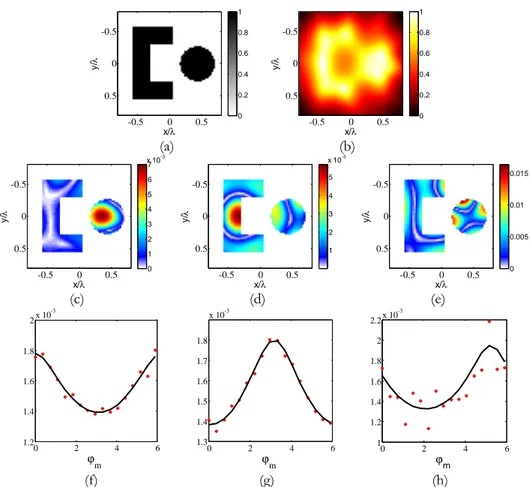
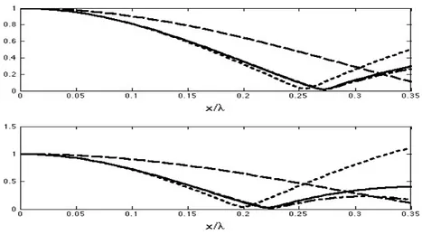
experiments: (a) actual support of the scattering system; (b) retrieved support via LSM energy indicator. Amplitude of virtual induced current for some sampling points: (c) =(0.388 λ, -0.0125 λ), (d) =(-0.413 λ, -0.0125 λ), (e) =(0.288 λ, -0.513 λ). Fitting of LSM equation versus [rad] for the pivot points considered in (c), (d) and (e), respectively: continuous line represents the values assumed by the right hand side while the red points are the values assumed by the left hand side. ... 32 Figure 2.1 Behavior of the Bessel function amplitude (solid line) as compared

to the approximation (2.4) truncated at the first term (dashed line), at the second term (dotted line) and at the third term (dash-dot line). Two complex contrast values are reported: in the upper panel = 1 − 0.05 , while in the lower one = 2 − 0.1 . The background medium is lossless. ... 45 Figure 2.2. Numerical assessment of DARE. The circular homogeneous

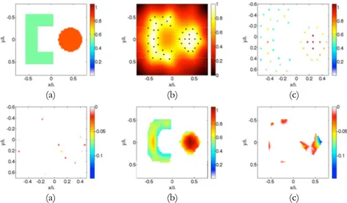
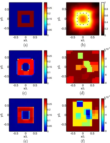
target: (a) real part of the reference profile; (b) LSM indicator map with the selected pivot points superimposed as dots; (c) real part and (d) imaginary part of punctual value of retrieved contrast, before interpolation; (e) real part and (f) imaginary part of retrieved contrast. ... 52 Figure 2.3. Numerical assessment of DARE. The C-O target: (a) real part of

the reference profile; (b) LSM indicator with the selected pivot points superimposed as dots; (c) real part and (d) imaginary part of punctual value of retrieved contrast, before interpolation; (e) real part and (f) imaginary part of retrieved contrast. ... 52 Figure 2.4. Numerical assessment of RCSI. The ring-shaped scatterer. (a) Real

part and (b) imaginary part of the contrast profile; (c) Normalized logarithmic LSM indicator map with the selected pivot points superimposed as dots; (d) visual sketch of the circular region ℐ for the innermost pivot point with a contour plot of the actual scatterer

support; (e) same as (d), but for the inner pivots; (f) same as (d), but for the outermost pivot points; (g) real part and (h) imaginary part of the retrieved contrast. ... 59 Figure 2.5 The Flowchart describing the DIVE method. ... 63 Figure 2.6. Numerical assessment of DIVE. The kite target: (a) real part and

(b) imaginary part of the reference profile. LSM indicator maps with the selected pivot points superimposed on it, for k=0 (e) and k=1 (h). Real part and imaginary part of the initial estimation (c)-(d) and of the final reconstruction (f)-(g). Real part and imaginary part of the retrieved contrast function with DBIM (i)-(j). The RRE versus iterations respectively for DIVE (k) and DBIM (l), respectively. ... 66 Figure 2.7. Validation of VE based methods with the Fresnel TwinDielTM

target data: (a) Reference profile. Real part and imaginary part of the retrieved contrast function with DARE (b)-(c), RCSI (d)-(e) and DIVE (f)-(i). In particular (f)-(g) is the initial estimation and (h)-(i) is the final reconstruction. ... 71 Figure 2.8. Validation of VE based methods with the Fresnel FoamDielIntTM

target data: (a) Reference profile. Real part and imaginary part of the retrieved contrast function with DARE (b)-(c), RCSI (d)-(e) and DIVE (f)-(i). In particular (f)-(g) is the initial estimation and (h)-(i) is the final reconstruction. ... 72 Figure 2.9. Validation of VE based methods with the Fresnel

FoamTwinDielIntTM target data: (a) Reference profile. Real part and

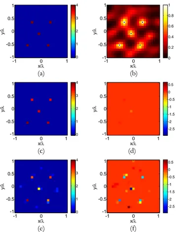
imaginary part of the retrieved contrast function with RCSI (b)-(c) and DIVE (d)-(g). In particular (d)-(e) is the initial estimation and (f)-(g) is the final reconstruction. ... 73 Figure 3.1. Numerical assessment of CS linearized approaches. The five

lossless point-like scatterers. (a) Actual contrast profile. (b) LSM indicator map with the selected pivot points superimposed as dots. Contrast profile retrieved profile via the approach (3.5) (c) real and (d) imaginary part. The retrieved profile with approach (3.5) cast for just the virtual incident fields: (e) real and (f) imaginary part. ... 89 Figure 3.2. Numerical assessment of CS linearized approaches. The three

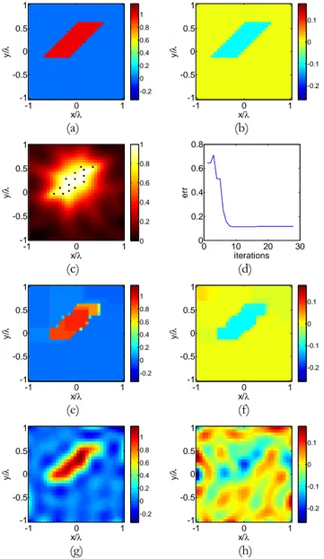
square target. (a) Actual contrast profile. (b) LSM indicator map with the selected pivot points superimposed as dots. The retrieved profile with approach (3.7): (c) real and (d) imaginary part. ... 89 Figure 3.3. Numerical assessment of CS linearized approaches. The slanted

square target. Contrast reference profile: (a) real part, (b) imaginary part. (c) LSM indicator map with the selected pivot points superimposed as dots. (d) The mean square error versus the number of iterations. The retrieved profile with approach (3.7): (e) real (f) imaginary part. The retrieved profile with TSVD: (g) real (h) imaginary part. ... 90 Figure 3.4. Numerical assessment of CS linearized approaches. The ring

square example. (a) Real part of the contrast reference profile. (b) LSM indicator map with the selected pivot points superimposed as dots. The retrieved profile by means of the approach (3.7): (c) real and (d) imaginary part. The retrieved profile by means of the

Figure 3.5 Plot of a generic monodimensional and non quadratic cost functional. The different local minima correspond to different attraction basins. ... 93 Figure 3.6. Numerical assessment of CS non linear approaches. The

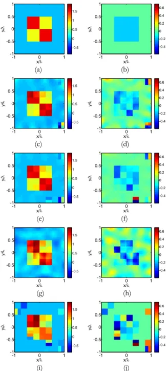
inhomogeneous square. (a) Real part and (b) imaginary part of the contrast reference profile. The retrieved profile with approach (3.12) ( = 150, err=5%): (c) real and (d) imaginary part. The retrieved profile with approach (3.12) ( = 100, err=4%): (e) real and (f) imaginary part. The retrieved profile with approach (3.12) and considering = = 14 ( = 150, err=7%): (g) real and (h) imaginary part. The retrieved profile with approach (3.12) and considering = = 11 ( = 150, err=16%): (i) real and (j) imaginary part. ... 97 Fig. 3.7. Numerical assessment of CS non linear approaches. The lossy

Austria profile. (a) Real part and (b) imaginary part of the contrast reference profile. The retrieved profile with approach (3.14) (k = 5 ∙ 10 − 8, err=15%): (c) real and (d) imaginary part. The retrieved profile with approach (3.14) and considering = = 16 (k = 5 ∙ 10 − 8, err=19%): (e) real and (f) imaginary part ... 98 Figure 3.8. Numerical assessment of DIVE-CS. The kite target: real part and

imaginary part of the retrieved contrast function at the initial step (a)-(b) and at the last iteration (c)-(d). The RRE versus iterations for DIVE-CS(e). ... 103 Figure 3.9. Validation of DIVE-CS with experimental data: the Fresnel

TwinDielTM target at 6 GHz: (a)-(b) real part and imaginary part of the retrieved contrast function. (c)-(d) are the same of (a)-(b) for reduced number of processed data. ... 104 Figure 3.10. Validation of DIVE-CS with experimental data: the Fresnel

FoamTwinDielIntTM target at 4 GHz: (a)-(b) real part and imaginary

part of the retrieved contrast function. (c)-(d) are the same of (a)-(b) for reduced number of processed data. ... 105 Figure 3.11. Validation of DIVE-CS with experimental data: the Fresnel

FoamDielIntTM target at 4 GHz. (a)-(b) Real part and imaginary part

of the retrieved contrast function. (c)-(d) are the same of (a)-(b) for reduced number of processed data. ... 106 Figure 4.1. Conceptual scheme of the differential measurements procedure

adopted in MNP enhanced MWI to extract the useful signal. ... 113 Figure 4.2. Measurement configuration adopted in the breast cancer MWI. 117 Figure 4.3 Transversal slices of the permittivity maps across the tumor for the

two considered breast phantoms derived from magnetic resonance images and taken from the Wisconsin University Repository [Zastrow

et al., 2008]: (a) Ph1, (b) Ph2. ... 117

Figure 4.4. Numerical assessment of CS inspired approach for MNP enhanced MWI. Transversal slices of the retrieved absolute value of the induced magnetic contrast (Ph1): (a) via unconstrained implementation (b) by means of the constrained one. The black line indicates the actual contour of the tumor. ... 121

Figure 4.5 Numerical assessment of CS inspired approach for MNP enhanced MWI. Transversal slice of the reconstructed magnetic contrast in when setting < _{! "#}. ... 121 Figure 4.6. Numerical assessment of CS inspired approach for MNP

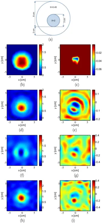
enhanced MWI. 3D Reconstructions of the absolute value of the induced magnetic contrast. (a) Ph1 and exact breast as reference scenario; (c) Ph1 and accurate reference breast; (e) Ph1 and empty system as reference profile; (b), (d) and (f) same as (a),(c) and (e) but for Ph2. ... 122 Figure 4.7. Numerical assessment of CS inspired approach for MNP

enhanced MWI. 3D Reconstructions of the absolute value of the induced magnetic contrast exploiting 12 probing and receiving antennas and considering the background as reference profile. (a) New measurements configuration; (b) reconstruction via CS and (c) via TSVD. ... 125 Figure 4.8. Numerical assessment of CS inspired approach for MNP

enhanced MWI. 3D Reconstructions of the absolute value of the induced magnetic contrast via CS (a) and via TSVD (b) (thresholded at -3dB). Transversal slices of the reconstructed differential magnetic contrast obtained via CS (c) and via TSVD (d). ... 126 Figure 5.1. The geometry of the 2D subsurface problem and the adopted

measurement configuration. The black circles and white triangles represent two or more transmitting and receiving antennas in a surface-GPR acquisition. ... 133 Figure 5.2. The virtual measurements setup. The black and white circles refer

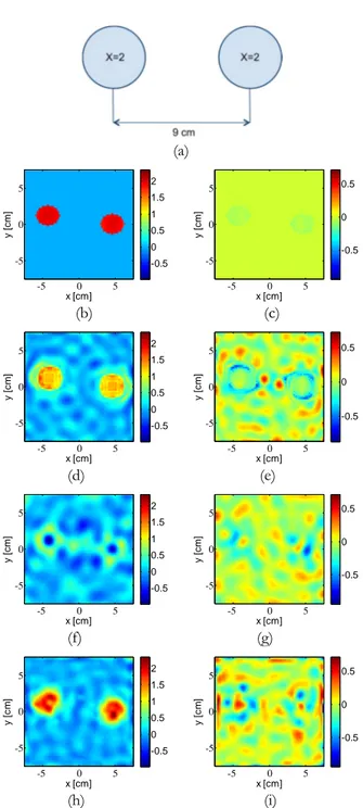
to actual and fictitious measurements, respectively, while the white triangles denote the transmitters. ... 136 Figure 5.3 Numerical assessment of VE-CS approach for subsurface MWI.

Example 1. (a) Logarithmic map of the LSM indicator with superimposed the pivot points and the contour of the reference profile, (b) virtual measurements setup. (c)-(d) Permittivity and conductivity of the retrieved profile by means of VE-CS ( = 0.18) for SNR=30dB ($ = 0.45, _"% = 0.29). ... 141 Figure 5.4 Numerical assessment of VE-CS approach for subsurface MWI.

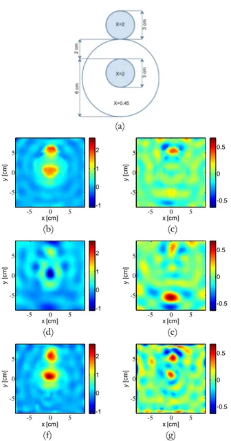
Example 2. (a) Logarithmic map of the LSM indicator with superimposed the pivot points and the contour of the reference profile, (b) virtual measurements setup. Permittivity and conductivity of the retrieved profile for SNR=30dB by means of (c)-(d) BA-CS ( & = 0.3) and (e)-(f) VE-CS ( & = 0.15). (g)-(h) the same as (e)-(f) for SNR=10dB with &= 0.17. ... 141 Figure 5.5 Numerical assessment of VE-CS approach for subsurface MWI.

Example 2. (a) Logarithmic map of the LSM indicator with superimposed the pivot points and the contour of the reference profile, (b) virtual measurements setup. Permittivity of the retrieved profile by means of the CS with (c) BA ( & = 0.04), (d) VE ( &= 0.32), (e)-(f) VE with RF=4 ( &= 0.28) and RF=10 ( &= 0.15), respectively for SNR=30dB. (g)-(j) the same as (c)-(f) for SNR=10dB with &=

0.26 (BA-CS), &= 0.33 (VE-CS), &= 0.28 (RF=4) and &= 0.24 (RF=10). ... 142 Figure E.1 CS ‘for dummies’. Sets defined by data equation for '_%= 3 and

')′ = 3 (a), 2 (b) and 1(c). ... 161

Figure E.2 CS ‘for dummies’. Sets defined by sparsity assumption for '_%= 3 and + = 2(a) and 1(b). ... 161 Figure E.3 CS ‘for dummies’. Intersections the sets determined by the data

equation and the sparsity assumption. ... 161 Figure E.4: CS ‘for dummies’. ℓ -balls for the cases p=3 (a), p=2 (b), p=1 (c)

and p=0.5 (d) ... 166 Figure E.5: CS ‘for dummies’. Intersection between ℓ_- - ball and data set. As

long as the data set is not parallel to any face or edge of the ℓ_- - ball solution to (C.6) is unique, and corresponds to the solution of the original intersection problem. ... 166

List of Tables

Table I. Numerical assessment of DIVE. The kite target: details of the inversion procedures. ... 65 Table II. The Fresnel TwinDielTM target: details of the inversion procedures.

... 71 Table III. The Fresnel FoamDielIntTM target: details of the inversion

procedures. ... 72 Table IV. The Fresnel FoamTwinDielIntTM target: details of the inversion

procedures. ... 73 Table V. Numerical assessment of DIVE-CS. The kite target: overall details

of the inversion procedures. ... 103 Table VI. The Fresnel TwinDielTM: overall details of the inversion

procedures. ... 104 Table VII. The Fresnel FoamTwinDielIntTM: overall details of the inversion

procedures. ... 105 Table VIII. The Fresnel FoamDielIntTM: overall details of the inversion

procedures. ... 106 Table IX. Numerical assessment of CS inspired approach for MNP enhanced MWI: polarizability and volumetric errors ... 123 Table X. Numerical assessment of VE-CS approach for subsurface MWI:

error metrics for the second example. ... 140 Table XI. Numerical assessment of VE-CS approach for subsurface MWI:

List of Acronyms

BA Born Approximation

BIM Born Iterative Method

CS Compressive Sensing

CSI Contrast Source Inversion

DARE Direct Algebraic Reconstruction

DBA Distorted Born Approximation

DBIM Distorted Born Iterative Method

DIVE Distorted Iterative Virtual Experiment

DOF Degree of Freedom

EPT Electric Properties Tomography

FFE Far Field Equation

FM Factorization Method

GPR Ground Penetrating Radar

LSM Linear Sampling Method

MNP Magnetic Nanoparticle

MR Multiplicative Regularization

MRI Magnetic Resonance Imaging

MWI Microwave Imaging

PMF Polarizing Magnetic Field

RCSI Regularized Contrast Source Inversion

RIP Restricted Isometry Property

ROI Region Of Interest

SNR Signal to Noise Ratio

SOM Subspace Optimization Method

SVD Singular Value Decomposition

TSVD Truncated Singular Value Decomposition

TV Total Variation

Introduction

I.1 Inverse scattering problems and their relevance

An electromagnetic field which is propagating in the space in presence of obstacles goes through some perturbations depending on their nature and features. This phenomenon, which is named electromagnetic scattering [Colton

and Kress, 1998, Hopcraft and Smith, 1992], implies the presence in the space of

a new electromagnetic field, known as total field, given by the linear superposition of the original one, which is called incident or unperturbed field, and the perturbation field, which is referred to as scattered field. The scattered field is physically generated by the targets that interact with the incident field during its propagation. In fact, the incident field induces inside the obstacles some currents which become sources of the scattered field.

Electromagnetic scattering implies two different classes of problems: forward scattering and inverse scattering. The forward scattering problem aims at determining the scattered field when the features of the targets which have generated it and the incident field are known. On the contrary, the inverse scattering problem consists in the quantitative reconstruction of the targets’ features starting from the knowledge of the incident field and the measurements of the scattered field [Colton and Kress, 1998, Hopcraft and Smith, 1992].

From a physical point of view, the difference between direct and inverse problem is linked to the concept of cause and effect. In the direct problem, starting from the knowledge of the causes (the interaction between the incident field and the objects) the aim is the computation of the scattered field, while the inverse scattering problem amounts at determining the feature of the targets which generate the perturbation of the original field, provided that the effect of the interaction (the scattered field) is known. These

Introduction

problems are related by a sort of duality, that is if the role of data and unknowns is exchanged one problem is obtained from the other one [Bertero

and Boccacci, 1998].

Although strictly coupled, the mathematical nature of the two problems is deeply different. In fact, the forward inverse scattering problem is linear and well posed, that is, according the Hadamard’s definition [Bertero, 1989], its solution always exists, is unique and depends continuously on the data, which are represented by the knowledge of the incident fields and the features of the obstacles. This is not true for the inverse scattering problem which is both non-linear and ill-posed with respect to the nature of the obstacles [Colton and

Kress, 1998, Hopcraft and Smith, 1992, Bertero and Boccacci, 1998]. Because of the

difficulty in tackling the ill-posedness and non-linearity of the problem, significant efforts have to be pursued in the mathematical, applied physics and engineering communities to develop reliable, effective and accurate methods and strategies to solve this inverse problem. However, such a challenging task is still an open issue.

Obviously, the availability of processing techniques able to avoid the difficulties due to non-linearity, as well as to give an accurate quantitative rendering of the actual electromagnetic scenario, is essential in a number of applications. Surely, the capability of microwaves of investigating non-accessible scenarios in a non-invasive and non-destructive way has contributed to increase the strong interest in applications [Pastorino, 2004], such as subsurface prospections [Daniels, 2004, Persico, 2014], biomedical diagnostics [Hassan and El-Shenawee, 2011, Semenov and Corfield, 2008, Semenov et

al., 2007], safety and security surveying operations [Pierri et al., 2013, Jin and Yarovoy, 2015, Millot and Casadebaig, 2015], and non-destructing testing of

materials [Zoughi, 2000], only to mention some examples.

Probably, one of the most important applications of microwave is in medical imaging, wherein this technology could improve health care in terms of prevention screening programs and monitoring applications.

In fact, in the last years the evidence that human tissues exhibit different electromagnetic properties at microwaves, depending on their

Microwave Imaging (MWI) for medical applications, by exploring in particular the possibility of retrieving morpho-functional images of the inspected anatomical structure. The use of non-ionizing radiations and possibly cheap and portable devices represents the main advantage offered by MWI with respect to other medical imaging techniques.

In particular, MWI has gained increasing interest in breast cancer diagnostics [Fear et al., 2002, Hassan and El-Shenawee, 2011], as it represents the first cause of death for cancer in women and its early diagnosis has a huge impact in the fight against cancer. Moreover, currently adopted diagnostic techniques in breast cancer diagnostic still suffer from some limitations and researchers are pushed to investigate to alternative techniques. For instance, the widely adopted X-ray mammography, besides being ionizing, still could give a larger rate of false negatives and false positives, so in many cases a breast biopsy is needed to verify the tumor diagnosis.

In addition, several research groups are investigating the possibility to use microwave techniques in other fields of medical imaging, such as possible diagnostic tools for brain stroke and ischemic disease [Scapaticci et al., 2012a,

Semenov and Corfield, 2008]. This is due to the fact that ischemic tissues show in

the microwave band different electric properties with respect to healthy tissues and that microwaves are particularly suitable to perform a continuous monitoring, since they are not harmful for the patient, being non- ionizing. Other possible applications are bone mineralization monitoring [Meaney et al., 2012, Zhou et al., 2010] and soft tissues imaging [Semenov et al., 2007].

Another important class of applications is use of microwave in subsurface inspection [Daniels, 2004, Crocco and Soldovieri, 2011, Persico, 2014,

Soldovieri and Crocco, 2011]. A very wide range of possibilities exists, the most

common being the safe and accurate location of the position of buried object (like pipes, utilities or potential hazards such as mine shafts and voids), the investigation of the reinforcement and condition of roads, bridges, and airport runways, the identification of structural integrity of buildings, the study of the environmental and geological conditions, or archaeological sites.

Demining is another important application [Daniels, 2006, Persico, 2014]. In particular, modern mines are customarily built with plastic materials with

Introduction

only little or even no metallic parts. Therefore, they are often hardly visible or completely invisible to a metal detector. In this context it is fundamental for the effectiveness of the survey and the safety of the people involved in it to provide all the details possibly available, that is the position and the depth, the size, the shape and the electromagnetic properties of the buried target, in such a way to avoid the occurrence of false negative (or false positive). In this respect, microwave tomographic approaches offer different tools which are able to produce reliable and easily interpretable images of the investigated scenarios. Notably, such a kind of outcomes is much more user friendly than the ones achieved by using standard GPR data processing.

Finally, the inverse scattering problems solution are also of interest in the design of filters, radiation elements and microwave devices [Bucci et al., 2005, Roberts, 1995, Song and Shin, 1985, Hakansson, 2007, Di Donato et al., 2014a], as some synthesis problems can be formulated in terms of retrieval problems. For example in [Di Donato et al., 2014a], an effective synthesis of cloaking profiles is performed via inverse scattering techniques.

I.2 Basic equations and approaches

The two fundamental equations describing the relevant scattering problem for a generic incident field ._/ are the data equation and the state equation. The first one is an integral representation of the scattered field in the region exterior to the investigation domain, while the state equation is the integral representation of the total field inside the investigation domain. The mathematical expressions of these latter, in case of nonmagnetic media, are, respectively:

.0 = 123 .4

(I.1) . = ./+ 1!3 .4

where .₀ and . are the scattered field outside the investigation domain and total field induced in the investigation domain, respectively, and is the contrast function which relates the electromagnetic features of the object and the ones of the host medium. 1₂ and 1_! are a short notation for the bilinear integral radiation operators relating the quantity . to the scattered field .₀ outside and inside the investigation domain, respectively. Note in the above equations the time harmonic factor $67{9:;} is assumed and dropped.

The inverse scattering problem aims at retrieving the unknown contrast χ from the scattered fields .0 measured on a generic curve of observation. As

stressed in the introduction, such a problem is non-linear respect to χ and ill-posed. The former circumstance descends from the dependence of the total field . on the unknown contrast function χ expressed by the state equation, while the latter from the compactness of the radiation operator 1_> [Bertero

and Boccacci, 1998], as described in the following section.

According to the above considerations, if +(χ, ._/ ) denote the nonlinear scattering operator relating the contrast and the arbitrary incident field to the corresponding scattered field, the inverse scattering problem is generally solved by seeking the global minimum of:

Φ( ) = ‖.0− +(χ, ./ )‖D

(I.3) which defines the discrepancy between the measured data and the predicted scattered field, corresponding to χ and ._/ [Roger, 1981, Joachimowicz et al., 1998]. An alternative approach involves the simultaneous solution of the system of equations (I.1)-(I.2) for both the contrast function and the electric field inside the object. Obviously, the set of unknowns enlarges but the degree of non linearity [Bucci et al., 2001a] reduces to that of a fourth order polynomial. In this case the problem is generally solved by seeking the global minimum of:

Φ( , .) = ‖.0− 123 .4‖D+ ‖.(E) − ./(E) + 1!3 .4‖D

Introduction

Finally, it is also possible to consider the currents induced inside the object as auxiliary unknowns instead of the total field .. To this end, the mathematical formulation of the problem is modified by defining the contrast sources F = .. Opposite to field-type approaches, in this case the inverse scattering problem is turned into an inverse source problem and one of the two fundamental equations of the electromagnetic scattering, i.e. the eq. (I.1), become linear [van den Berg and Kleinman, 1997, D’Urso et al., 2010, Isernia et al., 2004].

I.3 Two challenging difficulties: ill-posedness and

non-linearity

Besides its applicative relevance, the inverse scattering problems are also challenging from a theoretical point of view. Indeed, as pointed out in the previous Sections, the inverse scattering problem is ill-posed and also non-linear in the relationship between the data and unknowns.

A. Implication of ill-posedness

A problem is said well-posed according to the Hadamard’s definition [Bertero, 1989] if its solution always exists, it is unique, and it depends continuously on the data. If one of these three requirements is not satisfied, that is the solution might not exist at all, or it might not be unique or might not depend continuously on the data, then the problem is said to be ill-posed. This latter requirement is related to the ‘physical meaning’ of the solution. As a matter of fact, the key idea of Hadamard was to assume that an estimate of the unknown of the problem which considerably changes following a small variation of data is not a reliable solution. This has an immediate practical consequence, as variations on the data may occur (actually, occur) due to the unavoidable presence of measurement errors.

In inverse scattering problems the solution always exists, and theoretical uniqueness is proved in both tridimensional and bidimensional cases [Colton

and Paivarinta, 1992, Nachman, 1993]. The crucial point is represented by the

continuity requirement, as described in the following.

In case of single-view (a single illuminating incident wave is used), the scattering operator which relates unknown target’s properties to scattered fields is compact, i.e. it transforms any bounded set in a pre-compact one [Kolmogorov and Fomine, 1973, Bertero and Boccacci, 1998]. As the inverse of a compact operator cannot be continuous, the single view inverse scattering problem is ill-posed and small variations of the scattered field data produce unbounded variations of the corresponding ‘solutions’. The data are always affected by noise, which is then amplified in the inversion process, thus rendering completely meaningless the retrieved solution. This happens also in the discrete version of the inverse scattering problem, which is referred to as

ill-conditioned problem.

To get a better insight into the ill-posedness, it is worth recalling that another basic property of pre-compact sets is that they admit a finite-dimensional representation within any required accuracy [Kolmogorov and

Fomine, 1973, Bucci and Isernia, 1997]. Any scattered field can be accurately

represented with a finite number of parameters and such a number can be identified as the number of Degree Of Freedom (DOF) of the field [Bucci and

Franceschetti, 1989]. It follows that only a finite number of independent

measurements of the scattered field is available and hence only a limited number of independent parameters can be recovered from scattered field data. In fact, it is not possible to retrieve a generic function belonging to an infinite dimensional space from a finite number of parameters belonging to a finite dimensional space.

Unfortunately, also in case of multi-view cases (more illuminating incident waves are used) the problem remains ill-posed. The incident fields also belong to a compact set as non superdirective source are assumed, and, by considering the same arguments used in the single-view, the scattering operator is also compact in the multi-view case. Hence, there is no hope of extending at will the number of independent equations considering different incident fields. Only a finite number of scattering experiments can be in fact considered.

Introduction

As a consequence, the problem cannot be solved in any ordinary sense, but a generalized solution has been defined in order to restore well-posedness.

B. Implication of non-linearity

As shown in Section I.2, a generalized solution of inverse scattering is usually looked for by minimizing a suitable cost functional, which takes into account the physical model and also the relationship between the measured field data and the corresponding unknown contrast function.

Due to the non-linearity of the underlying problem, this cost functional is a non-quadratic one, so that it may have many local minima which are ‘false solutions’ of the problem [Isernia et al., 2001]. The more the problem departs from a linear one the more the occurrence of false solutions.

As a consequence, the obtained results depend on the considered initial guess. In fact, if the initial guess does not belong to the attraction region of the actual solution, the minimization scheme, if not adequately constrained, could be trapped in local minima, which could be completely different from the actual ground truth.

Moreover, the cost functional usually depends on a very large number of unknowns, especially in tridimensional geometries.

Besides the global optimization, which is often not viable in realistic case due to the elevate number of unknowns, several strategies do exist to tackle and defeat the occurrence of the false solutions and, so, to counteract the non-linearity. In the following Section, the main ones are briefly discussed.

I.4 Solution strategies

Due to the difficulty in tackling the non-linearity and ill-posedness of the inverse problem different efforts have been carried out in the literature.

A common feature for any inversion approach is the requirement to be fast, to have a low computational burden and to provide reliable

reconstructions with as minor as possible priori information on the physical or geometrical properties of the unknown scenario.

I.4.1 Regularization techniques

In order to restore well-posedness, the solution of the problem must fit the data within the experimental error but also expresses some expected physical properties of the unknown. The most simple form of enforce a priori information is to include a regularizing term in the cost functional.

The principle of the regularization methods is indeed to use the additional a priori information on the contrast function in an explicit way to construct from the beginning a solution both compatible with the data and which exhibit some specific physical features. The kind of additional information which can be exploited and/or enforced includes (but it is not limited to):

i. an upper bound on the dimensionality of the space where the unknown function is looked for. In order to avoid ill-posedness problem, a necessary (still not sufficient) condition is that its dimension is not greater than the one of the data space. Such a strategy can be defined ‘regularization by projection’ [Bucci et al., 2001b, Isernia et al., 1997, Isernia et al., 2004, Catapano et al., 2009a,

Scapaticci et al., 2012b, Scapaticci et al., 2015, Li et al., 2013, Lencrerot et al.,

2009];

ii. a requirement on the energy of the solution such as for instance a minimum ℓ_G energy requirement. This is the case of the well known Tikhonov regularization technique [Tikhonov et al., 1995, Bertero and

Boccacci, 1998];

iii. enforcing a piecewise constant behavior on the contrast function [Oliveri et al., 2014, van den Berg and Kleinman, 1995, van den Berg et al., 2003, Crocco and Isernia, 2001];

iv. physics induced bounds on the values of the unknown permittivity and conductivity functions (f.i., positive conductivities);

Introduction

v. the knowledge that the punctual value of the unknown function only can belong to a given finite alphabet of values [Catapano et al., 2004].

Strictly speaking, when dealing with the non-discretized problem, only (i), (ii) and (v) allow to hopefully restore well-posedness, as constraints (iii) and (iv) do not avoid to deal with infinite dimensional spaces for the unknown.

When the additional information is of statistical nature the regularized method are Bayesian.

In order to restore the well-posedness of the problem, another interesting opportunity is offered by the Compressive Sensing theory [Donoho, 2006, Baraniuk, 2007] (for more detail see Appendix E and Chapter 3), a new paradigm in signal recovery which is based on the concept of ‘sparsity’ or ‘compressibility’ of the unknown function, i.e the possibility to represent this latter in an exact or anyway accurate fashion through a limited number of nonzero coefficients of a convenient basis.

All the above discussed regularizations act only on the actual unknown that is the contrast function . When exploiting ‘contrast oriented’ regularization schemes, one is implicitly enforcing some property of the unknown function, and the effectiveness of the different regularizations will depend on how much the unknown scenario 'fits' the regularization model.

I.4.2 Traditional methods to overcome non linearity

As a countermeasure to non-linearity, linearized methods seem to allow a very easy implementation and require a limited amount of computer memory and computational time, even though they suffer from several limitations induced by the adopted approximated model.

In fact, considering for instance the Born Approximation (BA) [Devaney, 1984], the unknown total field inside the object is assumed equal to the incident field. This hypothesis is fully satisfied only in absence of the object itself so that the BA is acceptable in case of weak scatterers, i.e., for objects whose internal characteristics are very close to the ones of the external

medium, and/or for objects whose dimension is very small in terms of the wavelength in the external medium, so that the scattered field due to their presence is negligible with respect to the incident field. Note, if the linearization is performed around a nominal scenario different from a homogeneous background, the underlying approximation is referred to as Distorted Born approximation (DBA) [Devaney and Oristaglio, 1983].

Other examples of linearized methods are the physical optics approximation (Kirchhoff approximation), where waves are scattered from electrically large conductors, and the Rytov approximation, where the length scale of fluctuations is large as compared to the wavelength [Devaney, 1981].

These methods are quantitative, i.e. give the full characterization of the targets, as long as the adopted approximated model holds true. As a consequence, because of their limitations, they are typically not capable of providing an accurate description of the targets’ features when exploited outside of the range of validity of the underlying approximations and could give completely meaningfulness results.

As improvement with respect to the linearized method, the quadratic method [Brancaccio et al., 1995, Pierri et al., 2002] is also worth being mentioned. In this latter, a weak degree of non-linearity is introduced by adopting a second order approximation for the unknown-data mapping operator. In particular, the method is named quadratic as the unknown appears as a power of the second order. With respect to the linear methods as for instance BA, it allows to reconstruct a class of unknown profiles wider, but in any case it has a limited practical interest.

A possible extension of BA to the case of non-weak scatterer can be represented by the Born iterative method (BIM) [Wang and Chew, 1989] and the distorted Born iterative method (DBIM) [Chew and Wang, 1990]. This latter aims at solving the two coupled scattering integral equations by solving a sequence of linear problems and by updating the internal fields (also the Green function in DBIM) at each iteration through the solution of a forward scattering problem. Obviously, the final outcome and performances depend on the starting guess and the range of validity of the intermediate

Introduction

linearizations, so the convergence to actual ground truth cannot be always ensured.

In order to overcome the above limits, iterative optimization procedures, which tackle the inverse scattering problem in its full non linearity and do not involve any approximations, are often proposed to determine both the morphology and the electromagnetic contrast of the targets. The main practical difficulty with the iterative optimization algorithms is the long (or extremely long) reconstruction times required in order to complete the minimization. Global optimizations, as genetic or particle swarm algorithms [Haupt, 1995, Pastorino et al., 2000, Donelli et al., 2006], are generally not viable in case of large number of unknowns (typical in realistic problems like medical imaging) due to the exponential growth of the computational complexity.

For this reason, local iterative optimization schemes are usually adopted. Examples of these are the modified gradient method [Kleinman and van den

Berg, 1993, Souriau et al., 1996, Isernia et al., 1997, D’Urso et al., 2010], the

Contrast Source Inversion (CSI) method [van den Berg and Kleinman., 1997], the Contrast Source Extended Born model [Isernia et al., 2004] and the Subspace Optimization Method (SOM) [Chen, 2010]. However, being the cost functional related to the underlying problem non-linear, local minimization is prone to the occurrence of false solutions [Isernia et al., 2001].

Increasing as much as possible the essential dimension of data and reducing as much as possible the number of unknowns, positively affects the false solution problem. In fact each additional independent contribution will have a minimum in the actual solution, while its other minima will be widespread. The additional equations will fit the local minima as long as they are independent from the previous ones. For instance further data can be gained by multi-view scattering experiments, with the only drawback that the complexity of the image device increases. Unfortunately, at a given frequency only a finite amount of independent experiments can be performed (see Section I.3.A). An alternative possibility is offered by the frequency diversity, although it needs to model dispersive behavior of the involved media [Bucci et

Moreover, if appropriate a priori information is available, optimization methods can be equipped with a good starting guess, regularization schemes or constraints (see for instance the subsection I.4.1) in order to extend their applicability and reliability.

Additionally, in order to gain preliminary understanding of shape and/or of other characteristics of the unknown objects and overcome the limitations of optimization schemes and even linearized method [Catapano et

al., 2007a, Brignone et al., 2007], smart pre-processing techniques can be exploited

[Cakoni and Colton, 2006, Colton et al., 2003, Kirsch, 1998, Zhong and Chen, 2007,

Catapano et al., 2007b, Zhang et al., 2012a, Crocco et al., 2013].

Two relevant examples are the Linear Sampling Method (LSM) [Colton

et al., 2003, Catapano et al., 2007b] and the Factorization Method (FM) [Kirsch,

1999], which pursue the reconstruction of the morphological features of the scatterers by solving an auxiliary linear inverse problem with a negligible computational burden. For instance in [Catapano et al. 2007a] the target’s support estimation, obtained via LSM, is used for quantitative inversion carried out via non-linear optimization, thus improving the reliability of the inversion process and reducing its computational burden.

Finally, an interesting alternative to deal with the occurrence of the false solutions can be represented by step wise refinement techniques. Some examples include:

• frequency hopping techniques [Haddadin and Ebbini, 1998], in which, one starts with a low resolution reconstruction, by processing just the lower frequency data, and then uses it as a starting guess for higher frequency reconstruction. This technique plays a very important role, as low frequencies make it possible to locate the objects and to reconstruct them roughly, and then higher frequencies allow finer details to be retrieved;

• multiscale/multiresolution techniques [Baussard, 2005, Scapaticci et al., 2012b, Chiappinelli et al., 1999, Scapaticci et al., 2015], in which one starts with a coarse representation of the unknown and then improve reconstruction by focusing attention on details (in this respect Wavelets transform seem be a convenient framework);

Introduction

• the splitting of the problem into simpler auxiliary ones, each one devoted to determine some partial information about the scatterer (such as position of the center of the scatterer, presence of losses, possible symmetries, mean value and shape of its permittivity distribution), before the final quantitative inversion.

I.4.3 Some recent developments

As discussed in the previous subsection, a priori information on the unknown and pre-processing techniques are traditionally exploited in order to limit the occurrence of false solution. In fact, each preliminary knowledge on the unknown contrast can be used to get a good starting point for iterative inversion schemes in order to fall into the right attraction basin, or to restrict of the dimensionality of the unknown space, or choose the suitable representation basis in order to increase the data-unknown ratio (f.i. projection methods based on Fourier harmonics or Wavelets transform), or even to enforce other constraints.

On the other hand, priori information on the unknown or suitable pre-processing step could open the way to a new way of thinking about the solution of inverse scattering problems. In fact, rather than enforcing during the inversion procedure some properties, known a priori or acquired by means of a pre-processing of the data, one can take into account them from the beginning by rewriting the pertinent scattering equations [Isernia et al., 2004, Ma et al., 2000, Crocco et al., 2012a].

For instance in [Isernia et al., 2004] by taking advantage of the a priori information on the features of the Green's function, a convenient rewriting of the integral equations (I.1) and (I.2) has been exploited to introduce a new model for bidimensional electromagnetic scattering by dielectric objects in lossy media. By exploiting this latter, a new series expansion has been introduced in order to accurately and effectively solve the forward and inverse problem. This main advantage offered by this new scattering model is the lower degree of nonlinearity with respect to parameters embedding dielectric

A suitable rewriting of the scattering equation and a new field approximation, which rely on a proper (physics inspired) exploitation of the solution of the LSM, have been recently proposed in [Crocco et al., 2012a]. The proposed field approximation takes into account the nature of the unknown scenario through the pre-processing step and allows to exploit a linear model for quantitative reconstruction. In particular, in [Di Donato et al., 2015a] the range of applicability of this original inversion procedure is investigated showing that it significantly outperforms the usual BA, as it is target dependent and considers the contribution of the field scattered by the object. A generalized version of this linear inversion method has been recently introduced in [Di Donato et al., 2016] in order to appraise the properties of non-weak anomalies with respect to a partially known and non-homogeneous scenario, going beyond the range of validity of the DBA.

Other recent development in the solution of inverse scattering interests a new kind of regularization, which interest the auxiliary unknown, furtherly considered in addition to the actual one, rather than the contrast function (see subsection 1.4.1). Notably, enforcing some property on the auxiliary unknown would allow to reduce the nonlinearity of the inverse scattering problem, with obvious beneficial effects with respect to the possible occurrence of false solutions.

Note the only method up to now acting on the contrast sources to regularize the problem is the subspace optimization method (SOM) [Chen, 2010]. The essence of the method is that part of the contrast source is determined from the spectrum analysis without using any optimization, whereas the rest is determined by optimization method.

The intrinsically different nature of these regularizations, with respect to other ones acting on the contrast, naturally suggests that these approaches could be exploited together, leading to further improved performances, as done in [Xu et al., 2015].

Introduction

I.5 Aim and outline of the thesis

Solutions of inverse scattering problems can be completely erroneous if non-linearity and ill-posedness are not properly tackled. The availability of processing techniques, able to avoid the possible occurrence of false solutions as well as able to give an accurate quantitative rendering of the actual electromagnetic scenario, is essential in several applications (such as demining and biomedical imaging), as discussed in the Section I.1.

In this respect, the aim of the thesis is concerned with the development of innovative and reliable solution procedure for quantitative inverse scattering problem, which have a range of applicability as wide as possible while keep low both the complexity of the solution method and the computational burden.

In this thesis the 2D problem is analyzed and discussed, as its full understanding is still an open issue and is pivotal towards the more demanding 3D case. In fact, both the optimization of the corresponding inversion approaches and the possibility of using interesting high performance hardware resources and effective solution strategies allow to foresee a simple extension at the case of 3D geometry. As a demonstration of the actual viability in 3D problems, in Chapter 5, a tridimensional geometry is also considered.

With the aim of developing new solution strategies and tools, the general idea of the thesis is the well-conditioning of the inverse scattering problem by acting from one hand on the actual variable, that is the contrast function, and from the other hand on the auxiliary unknown, that is the total field or the contrast sources induced inside the target.

In order to act on the auxiliary unknown and contemporary reduce the non-linearity, in the first part of the thesis the new paradigm of Virtual

Scattering Experiments (VE) is introduced. VE are a new kind of

experiments, which are obtained starting from the statement that scattering phenomena can be recombined in many different ways, due to the linearity of Maxwell equations with respect to the primary sources. Their peculiarity is that they can be designed in such a way to condition the scattering

phenomena and enforce some peculiar properties on the internal fields or on the corresponding currents. Note that this kind of information does not descend from some priori assumptions on the scattering model or on the contrast function. Rather, it follows from some smart pre-processing of the available data. In particular, in this thesis, such information is conveniently used in order to develop three new inversion approaches (see Chapter 2 and [Bevacqua et al., 2014a, Bevacqua et al., 2015a-d]).

On the contrary, in order to act on the actual unknown, the emerging and powerful tool in signal/image processing of the Compressive Sensing is exploited. The CS allows to improve the accuracy of existing inversion procedures, obtaining a kind of ‘super- resolution’, and/or driving the design of simpler and cheaper measurement set-ups. Obviously, it can be definitely attractive in the solution of inverse scattering problems. Unfortunately, this theory is well developed only for the case of phenomena described through linear models. This represents a fundamental difficulty for its application in the problem at hand. In this respect, three different approaches are developed, in which a possible linearization is considered and discussed and two possible approaches considering the problem in its full non linearity are also explored [Di Donato et al., 2014b, Bevacqua et al., 2015e]

The thesis consists of 5 chapters and 5 appendices (where mathematical details are deepened) and it is organized in two different parts. In the first part of the thesis (Chapters 1-3) both theoretical and numerical results reached by developing innovative solution strategies for quantitative inverse scattering are illustrated and discussed. In the second part of the thesis (Chapters 4-5) the outcomes reached in the previous Chapters are originally exploited in order to improve the imaging results by considering two different applications: biomedical diagnostics, in particular for the breast cancer, and subsurface prospections. [Bevacqua and Scapaticci, 2015, Bevacqua et al., 2015f].

In particular, in Chapter 1, the mathematical notations and the general adopted measurement setup for 2D scalar problems are first illustrated. Then, the new paradigm of VE for the solution of inverse scattering problem is introduced and the possibility of conditioning the scattering phenomenon by means of proper designed VE is presented. To this end, the LSM is proposed

Introduction

as design tool [Crocco et al., 2011,Di Donato et al., 2011], by taking advantage of

its physical interpretation in terms of electromagnetic focusing problem. Finally, in light of the above field conditioning concept and the VE framework, two inversion methods recently introduced in literature are briefly recalled and reinterpreted. These strategies aim at counteracting the non-linearity of inverse scattering problem [Crocco et al., 2012a], and overcoming the relevant information lack arising when data are gathered under aspect limited measurements configuration [Di Donato and Crocco, 2015].

Chapter 2 introduces, describes and discusses three different solution strategies based on suitably designed VE. In particular, in the first two of them VE are built in such a way to induce a circularly symmetric behavior of the scattered fields and contrast sources. Then, limitations associated to the linearization used in [Crocco et al., 2012a] are overcome according to two different approaches.

In the first one, named Direct Algebraic Reconstruction (DARE) a new and original approximation of the contrast source induced inside the targets is introduced [Bevacqua et al., 2015g]. These latter allows to reduce the solution of the inverse problem to a diagonal system of third degree algebraic equations. This method provides a very fast solution of the inverse scattering problem by means of closed form formulas. The method is introduced and discussed in Section 2.1, while some details are deferred to Appendices A, B and C.

In Section 2.2, by using the same kind of VE, a Regularized Contrast Source Inversion (RCSI) scheme is introduced [Di Donato et al., 2015b], in which no approximation of the scattering model is considered. Rather, a simple regularization term acting on the induced currents rather than the contrast function is added in the standard CSI scheme. Some details about CSI scheme are reported in Appendix D.

In the same spirit of overcoming limitations due to linearizations or approximations, as well as to deal with scatterers located in a possibly non homogeneous background, in Section 2.3 a Distorted Iterated Virtual Experiments (DIVE) inversion method is discussed [Bevacqua et al., 2016a]. In

intermediate linearizations, in which the Green’s function, the VE and corresponding approximations [Crocco et al., 2012a] are updated on the basis of intermediate results.

While Chapter 2 is focused on VE as a way to have a conditioning of the auxiliary unknown H or I, Chapter 3 is concerned with the exploitation of possible regularizations on the contrast function. In particular, it introduces and describes new inversion methods inspired to CS theory, in which different possible kinds of sparsity of the contrast function, as well as different possible ways of exploiting them, are considered.

In particular, in Section 3.2 and 3.4 the CS theory is used in conjunction with VE based approaches [Bevacqua et al., 2015h, Bevacqua and Di Donato, 2015], that are the linear approximation recalled in Section 1.6.1, and the DIVE method introduced in Section 2.3. As such, these two methods act contemporary on actual unknown, which is supposed to be sparse, and on the auxiliary one, which is conditioned by means of well-designed VE.

Later in Section 3.3, a first attempt of imposing sparsity regularization in non-linear framework is discussed [Bevacqua et al., 2014b]. In particular, two innovative sparsity promoting methods are introduced and developed, which tackle the inverse scattering problem in its full non-linearity by adopting again a CSI scheme.

As a byproduct, an original geometrical interpretation of CS ‘for dummies’ is also furnished in Appendix E.

Both in Chapter 2 and 3, numerical results against simulated and experimental data are given in order to assess the validity of the proposed inversion methods.

As a proof of the actual viability of the introduced techniques in real applications, the second part of the thesis concerns with use of microwaves for the breast cancer imaging enhanced by the use of Magnetic Nanoparticles (MNP) and for the imaging of objects buried in the subsoil.

More in details, MNP enhanced MWI represents an innovative technique for breast cancer diagnosis, in which MNP have been proposed as contrast agent, in order to overcome some limitations of conventional microwave imaging techniques, thus providing reliable and specific diagnosis

Introduction

of breast cancer. In particular in Chapter 4 an ad hoc CS inspired inversion technique is introduced for the reconstruction of the magnetic contrast induced within the tumor [Bevacqua and Scapaticci, 2016].

On the other hand, the Subsurface MWI represents an assessed means to process GPR and valid alternative to the standard GPR data processing. In particular in Chapter 5, an efficient inverse scattering strategy based on framework of the VE and Compressive Sensing is proposed to achieve dielectric characterization of non-weak and extended hidden targets and buried objects in lossy soil [Bevacqua et al., 2016b].

Conclusions and recommendation for further developments are finally given.

Part I

NEW PARADIGM AND TOOLS FOR NON

LINEAR INVERSE SCATTERING

1

Conditioning scattering phenomena by

Virtual Experiments

1.1 Mathematical notations and measurement configuration

In the following the mathematical formulation of inverse scattering problems is introduced in more details with respect to the canonical 2D scalar case, by considering TM polarized fields, and assuming and dropping the time harmonic factor $67{9:;}.

The adopted measurements configuration is the so-called multiview-multistatic one, in which the antennas are organized in such a way that for each transmitting antenna all the antennas (including the transmitting one) act as receivers, and all antennas alternately act as a transmitter. By the sake of simplicity, let us consider the case where antennas are located in the far-field with respect to the investigation domain Ω ⊆ ℛG and on a circumference Γ

distant R from the origin of the reference system 6NO, which is centered respect to Ω, see fig. 1.1.

Let us consider an unknown nonmagnetic object with compact, possibly not connected support Σ and denote with Q_R and _S its relative permittivity and the electric conductivity, respectively. The target is embedded in a nonmagnetic medium of permittivity Q_T and conductivity _T. The magnetic permeability is everywhere equal to that of free space U_V.

The unknown contrast function which relates the electromagnetic features of the object and the ones of the host medium is defined in E = (6, O) ∈ Ω as :

(E) =_QQR(E) − 9 R(E) :Q⁄ V

T(E) − 9 T(E) :Q⁄ V− 1

Conditioning scattering phenomena by Virtual Experiments

where : = 2YZ and Z is the working frequency.

Figure 1.1 Pictorial view of the measurement configuration adopted to collect the scattering

experiments.

The equations governing the scattering phenomenon for the geometry at hand for the generic [ -th incident field H_!( ) can be expressed in an integral form as it follows:

HR( )(E) = \TG] ^T(E, E_) ` (E_<sub>)H</sub>( )<sub>(E</sub>_<sub>)aE</sub>_<sub>= 12b H</sub>( )<sub>c, E ∈ Γ</sub> (1.2) H( )<sub>(E) = H</sub> !( )(E) + \TG] ^T(E, E_) ` (E__)H( )_(E__)aE_ = H_!( )+ 1_!b H( )_{c, E ∈ Ω} (1.3) where H_R( )(∙) and H( )(∙) are the scattered field and total field induced in Ω, respectively, while \_T = :dU_TQ_T is the wavenumber in the host medium.1₂ and 1_! are a short notation for the bilinear integral radiation operators, which are defined on X × T, with X ⊂ ij(Ω) the subspace of the possible contrast functions, T ⊂ iG(Ω) a proper subspace for the total electric fields inside the object, and with value on two proper subspace for the scattered field outside and inside the object, S₂ ⊂ iG(Γ) and S_! ⊂ iG(Ω), respectively. ^_T(E, E_) is