arXiv:1712.02365v1 [astro-ph.HE] 6 Dec 2017
doi: 10.1093/pasj/xxx000
Hitomi Observations of the LMC SNR N132D:
Highly Redshifted X-ray Emission from Iron
Ejecta
∗
Hitomi Collaboration, Felix A
HARONIAN1,2,3, Hiroki A
KAMATSU4, Fumie
A
KIMOTO5, Steven W. A
LLEN6,7,8, Lorella A
NGELINI9, Marc A
UDARD10,
Hisamitsu A
WAKI11, Magnus A
XELSSON12, Aya B
AMBA13,14, Marshall W.
B
AUTZ15, Roger B
LANDFORD6,7,8, Laura W. B
RENNEMAN16, Gregory V.
B
ROWN17, Esra B
ULBUL15, Edward M. C
ACKETT18, Maria C
HERNYAKOVA1,
Meng P. C
HIAO9, Paolo S. C
OPPI19,20, Elisa C
OSTANTINI4, Jelle
DEP
LAA4,
Cor P.
DEV
RIES4, Jan-Willem
DENH
ERDER4, Chris D
ONE21, Tadayasu
D
OTANI22, Ken E
BISAWA22, Megan E. E
CKART9, Teruaki E
NOTO23,24, Yuichiro
E
ZOE25, Andrew C. F
ABIAN26, Carlo F
ERRIGNO10, Adam R. F
OSTER16,
Ryuichi F
UJIMOTO27, Yasushi F
UKAZAWA28, Akihiro F
URUZAWA29,
Massimiliano G
ALEAZZI30, Luigi C. G
ALLO31, Poshak G
ANDHI32, Margherita
G
IUSTINI4, Andrea G
OLDWURM33,34, Liyi G
U4, Matteo G
UAINAZZI35, Yoshito
H
ABA36, Kouichi H
AGINO37, Kenji H
AMAGUCHI9,38, Ilana M. H
ARRUS9,38,
Isamu H
ATSUKADE39, Katsuhiro H
AYASHI22,40, Takayuki H
AYASHI40, Kiyoshi
H
AYASHIDA41, Junko S. H
IRAGA42, Ann H
ORNSCHEMEIER9, Akio H
OSHINO43,
John P. H
UGHES44, Yuto I
CHINOHE25, Ryo I
IZUKA22, Hajime I
NOUE45,
Yoshiyuki I
NOUE22, Manabu I
SHIDA22, Kumi I
SHIKAWA22, Yoshitaka
I
SHISAKI25, Masachika I
WAI22, Jelle K
AASTRA4,46, Tim K
ALLMAN9,
Tsuneyoshi K
AMAE13, Jun K
ATAOKA47, Satoru K
ATSUDA48, Nobuyuki
K
AWAI49, Richard L. K
ELLEY9, Caroline A. K
ILBOURNE9, Takao
K
ITAGUCHI28, Shunji K
ITAMOTO43, Tetsu K
ITAYAMA50, Takayoshi
K
OHMURA37, Motohide K
OKUBUN22, Katsuji K
OYAMA51, Shu K
OYAMA22,
Peter K
RETSCHMAR52, Hans A. K
RIMM53,54, Aya K
UBOTA55, Hideyo
K
UNIEDA40, Philippe L
AURENT33,34, Shiu-Hang L
EE23, Maurice A.
L
EUTENEGGER9,38, Olivier L
IMOUSIN34, Michael L
OEWENSTEIN9,56, Knox S.
L
ONG57, David L
UMB35, Greg M
ADEJSKI6, Yoshitomo M
AEDA22, Daniel
M
AIER33,34, Kazuo M
AKISHIMA58, Maxim M
ARKEVITCH9, Hironori
M
ATSUMOTO41, Kyoko M
ATSUSHITA59, Dan M
CC
AMMON60, Brian R.
M
CN
AMARA61, Missagh M
EHDIPOUR4, Eric D. M
ILLER15, Jon M. M
ILLER62,
Shin M
INESHIGE23, Kazuhisa M
ITSUDA22, Ikuyuki M
ITSUISHI40, Takuya
M
IYAZAWA63, Tsunefumi M
IZUNO28,64, Hideyuki M
ORI9, Koji M
ORI39, Koji
M
UKAI9,38, Hiroshi M
URAKAMI65, Richard F. M
USHOTZKY56, Takao
N
AKAGAWA22, Hiroshi N
AKAJIMA41, Takeshi N
AKAMORI66, Shinya
N
AKASHIMA58, Kazuhiro N
AKAZAWA13,14, Kumiko K. N
OBUKAWA67,
Masayoshi N
OBUKAWA68, Hirofumi N
ODA69,70, Hirokazu O
DAKA6, Takaya
cO
HASHI25, Masanori O
HNO28, Takashi O
KAJIMA9, Naomi O
TA67, Masanobu
O
ZAKI22, Frits P
AERELS71, St ´ephane P
ALTANI10, Robert P
ETRE9, Ciro
P
INTO26, Frederick S. P
ORTER9, Katja P
OTTSCHMIDT9,38, Christopher S.
R
EYNOLDS56, Samar S
AFI-H
ARB72, Shinya S
AITO43, Kazuhiro S
AKAI9, Toru
S
ASAKI59, Goro S
ATO22, Kosuke S
ATO59, Rie S
ATO22, Toshiki S
ATO25,
Makoto S
AWADA73, Norbert S
CHARTEL52, Peter J. S
ERLEMTSOS9, Hiromi
S
ETA25, Megumi S
HIDATSU58, Aurora S
IMIONESCU22, Randall K. S
MITH16,
Yang S
OONG9, Łukasz S
TAWARZ74, Yasuharu S
UGAWARA22, Satoshi
S
UGITA49, Andrew S
ZYMKOWIAK20, Hiroyasu T
AJIMA5, Hiromitsu
T
AKAHASHI28, Tadayuki T
AKAHASHI22, Shin’ichiro T
AKEDA63, Yoh T
AKEI22,
Toru T
AMAGAWA75, Takayuki T
AMURA22, Takaaki T
ANAKA51, Yasuo
T
ANAKA76,22, Yasuyuki T. T
ANAKA28, Makoto S. T
ASHIRO77, Yuzuru
T
AWARA40, Yukikatsu T
ERADA77, Yuichi T
ERASHIMA11, Francesco
T
OMBESI9,78,79, Hiroshi T
OMIDA22, Yohko T
SUBOI48, Masahiro T
SUJIMOTO22,
Hiroshi T
SUNEMI41, Takeshi Go T
SURU51, Hiroyuki U
CHIDA51, Hideki
U
CHIYAMA80, Yasunobu U
CHIYAMA43, Shutaro U
EDA22, Yoshihiro U
EDA23,
Shin’ichiro U
NO81, C. Megan U
RRY20, Eugenio U
RSINO30, Shin
W
ATANABE22, Norbert W
ERNER82,83,28, Dan R. W
ILKINS6, Brian J.
W
ILLIAMS57, Shinya Y
AMADA25, Hiroya Y
AMAGUCHI9,56, Kazutaka
Y
AMAOKA5,40, Noriko Y. Y
AMASAKI22, Makoto Y
AMAUCHI39, Shigeo
Y
AMAUCHI67, Tahir Y
AQOOB9,38, Yoichi Y
ATSU49, Daisuke Y
ONETOKU27, Irina
Z
HURAVLEVA6,7, Abderahmen Z
OGHBI62,
1Dublin Institute for Advanced Studies, 31 Fitzwilliam Place, Dublin 2, Ireland 2Max-Planck-Institut f ¨ur Kernphysik, P.O. Box 103980, 69029 Heidelberg, Germany 3Gran Sasso Science Institute, viale Francesco Crispi, 7 67100 L’Aquila (AQ), Italy
4SRON Netherlands Institute for Space Research, Sorbonnelaan 2, 3584 CA Utrecht, The Netherlands
5Institute for Space-Earth Environmental Research, Nagoya University, Furo-cho, Chikusa-ku, Nagoya, Aichi 464-8601
6Kavli Institute for Particle Astrophysics and Cosmology, Stanford University, 452 Lomita Mall, Stanford, CA 94305, USA
7Department of Physics, Stanford University, 382 Via Pueblo Mall, Stanford, CA 94305, USA 8SLAC National Accelerator Laboratory, 2575 Sand Hill Road, Menlo Park, CA 94025, USA 9NASA, Goddard Space Flight Center, 8800 Greenbelt Road, Greenbelt, MD 20771, USA 10Department of Astronomy, University of Geneva, ch. d’ ´Ecogia 16, CH-1290 Versoix,
Switzerland
11Department of Physics, Ehime University, Bunkyo-cho, Matsuyama, Ehime 790-8577 12Department of Physics and Oskar Klein Center, Stockholm University, 106 91 Stockholm,
Sweden
13Department of Physics, The University of Tokyo, 7-3-1 Hongo, Bunkyo-ku, Tokyo 113-0033 14Research Center for the Early Universe, School of Science, The University of Tokyo, 7-3-1
Hongo, Bunkyo-ku, Tokyo 113-0033
15Kavli Institute for Astrophysics and Space Research, Massachusetts Institute of Technology, 77 Massachusetts Avenue, Cambridge, MA 02139, USA
16Smithsonian Astrophysical Observatory, 60 Garden St., MS-4. Cambridge, MA 02138, USA 17Lawrence Livermore National Laboratory, 7000 East Avenue, Livermore, CA 94550, USA 18Department of Physics and Astronomy, Wayne State University, 666 W. Hancock St, Detroit,
MI 48201, USA
19Department of Astronomy, Yale University, New Haven, CT 06520-8101, USA 20Department of Physics, Yale University, New Haven, CT 06520-8120, USA
21Centre for Extragalactic Astronomy, Department of Physics, University of Durham, South Road, Durham, DH1 3LE, UK
22Japan Aerospace Exploration Agency, Institute of Space and Astronautical Science, 3-1-1 Yoshino-dai, Chuo-ku, Sagamihara, Kanagawa 252-5210
23Department of Astronomy, Kyoto University, Kitashirakawa-Oiwake-cho, Sakyo-ku, Kyoto 606-8502
24The Hakubi Center for Advanced Research, Kyoto University, Kyoto 606-8302
25Department of Physics, Tokyo Metropolitan University, 1-1 Minami-Osawa, Hachioji, Tokyo 192-0397
26Institute of Astronomy, University of Cambridge, Madingley Road, Cambridge, CB3 0HA, UK 27Faculty of Mathematics and Physics, Kanazawa University, Kakuma-machi, Kanazawa,
Ishikawa 920-1192
28School of Science, Hiroshima University, 1-3-1 Kagamiyama, Higashi-Hiroshima 739-8526 29Fujita Health University, Toyoake, Aichi 470-1192
30Physics Department, University of Miami, 1320 Campo Sano Dr., Coral Gables, FL 33146, USA
31Department of Astronomy and Physics, Saint Mary’s University, 923 Robie Street, Halifax, NS, B3H 3C3, Canada
32Department of Physics and Astronomy, University of Southampton, Highfield, Southampton, SO17 1BJ, UK
33Laboratoire APC, 10 rue Alice Domon et L ´eonie Duquet, 75013 Paris, France 34CEA Saclay, 91191 Gif sur Yvette, France
35European Space Research and Technology Center, Keplerlaan 1 2201 AZ Noordwijk, The Netherlands
36Department of Physics and Astronomy, Aichi University of Education, 1 Hirosawa, Igaya-cho, Kariya, Aichi 448-8543
37Department of Physics, Tokyo University of Science, 2641 Yamazaki, Noda, Chiba, 278-8510
38Department of Physics, University of Maryland Baltimore County, 1000 Hilltop Circle, Baltimore, MD 21250, USA
39Department of Applied Physics and Electronic Engineering, University of Miyazaki, 1-1 Gakuen Kibanadai-Nishi, Miyazaki, 889-2192
40Department of Physics, Nagoya University, Furo-cho, Chikusa-ku, Nagoya, Aichi 464-8602 41Department of Earth and Space Science, Osaka University, 1-1 Machikaneyama-cho,
Toyonaka, Osaka 560-0043
42Department of Physics, Kwansei Gakuin University, 2-1 Gakuen, Sanda, Hyogo 669-1337 43Department of Physics, Rikkyo University, 3-34-1 Nishi-Ikebukuro, Toshima-ku, Tokyo
171-8501
44Department of Physics and Astronomy, Rutgers University, 136 Frelinghuysen Road, Piscataway, NJ 08854, USA
45Meisei University, 2-1-1 Hodokubo, Hino, Tokyo 191-8506
46Leiden Observatory, Leiden University, PO Box 9513, 2300 RA Leiden, The Netherlands 47Research Institute for Science and Engineering, Waseda University, 3-4-1 Ohkubo,
Shinjuku, Tokyo 169-8555
48Department of Physics, Chuo University, 1-13-27 Kasuga, Bunkyo, Tokyo 112-8551
49Department of Physics, Tokyo Institute of Technology, 2-12-1 Ookayama, Meguro-ku, Tokyo 152-8550
51Department of Physics, Kyoto University, Kitashirakawa-Oiwake-Cho, Sakyo, Kyoto 606-8502
52European Space Astronomy Center, Camino Bajo del Castillo, s/n., 28692 Villanueva de la Ca ˜nada, Madrid, Spain
53Universities Space Research Association, 7178 Columbia Gateway Drive, Columbia, MD 21046, USA
54National Science Foundation, 4201 Wilson Blvd, Arlington, VA 22230, USA
55Department of Electronic Information Systems, Shibaura Institute of Technology, 307 Fukasaku, Minuma-ku, Saitama, Saitama 337-8570
56Department of Astronomy, University of Maryland, College Park, MD 20742, USA 57Space Telescope Science Institute, 3700 San Martin Drive, Baltimore, MD 21218, USA 58Institute of Physical and Chemical Research, 2-1 Hirosawa, Wako, Saitama 351-0198 59Department of Physics, Tokyo University of Science, 1-3 Kagurazaka, Shinjuku-ku, Tokyo
162-8601
60Department of Physics, University of Wisconsin, Madison, WI 53706, USA
61Department of Physics and Astronomy, University of Waterloo, 200 University Avenue West, Waterloo, Ontario, N2L 3G1, Canada
62Department of Astronomy, University of Michigan, 1085 South University Avenue, Ann Arbor, MI 48109, USA
63Okinawa Institute of Science and Technology Graduate University, 1919-1 Tancha, Onna-son Okinawa, 904-0495
64Hiroshima Astrophysical Science Center, Hiroshima University, Higashi-Hiroshima, Hiroshima 739-8526
65Faculty of Liberal Arts, Tohoku Gakuin University, 2-1-1 Tenjinzawa, Izumi-ku, Sendai, Miyagi 981-3193
66Faculty of Science, Yamagata University, 1-4-12 Kojirakawa-machi, Yamagata, Yamagata 990-8560
67Department of Physics, Nara Women’s University, Kitauoyanishi-machi, Nara, Nara 630-8506
68Department of Teacher Training and School Education, Nara University of Education, Takabatake-cho, Nara, Nara 630-8528
69Frontier Research Institute for Interdisciplinary Sciences, Tohoku University, 6-3 Aramakiazaaoba, Aoba-ku, Sendai, Miyagi 980-8578
70Astronomical Institute, Tohoku University, 6-3 Aramakiazaaoba, Aoba-ku, Sendai, Miyagi 980-8578
71Astrophysics Laboratory, Columbia University, 550 West 120th Street, New York, NY 10027, USA
72Department of Physics and Astronomy, University of Manitoba, Winnipeg, MB R3T 2N2, Canada
73Department of Physics and Mathematics, Aoyama Gakuin University, 5-10-1 Fuchinobe, Chuo-ku, Sagamihara, Kanagawa 252-5258
74Astronomical Observatory of Jagiellonian University, ul. Orla 171, 30-244 Krak ´ow, Poland 75RIKEN Nishina Center, 2-1 Hirosawa, Wako, Saitama 351-0198
76Max-Planck-Institut f ¨ur extraterrestrische Physik, Giessenbachstrasse 1, 85748 Garching , Germany
77Department of Physics, Saitama University, 255 Shimo-Okubo, Sakura-ku, Saitama, 338-8570
78Department of Physics, University of Maryland Baltimore County, 1000 Hilltop Circle, Baltimore, MD 21250, USA
79Department of Physics, University of Rome “Tor Vergata”, Via della Ricerca Scientifica 1, I-00133 Rome, Italy
80Faculty of Education, Shizuoka University, 836 Ohya, Suruga-ku, Shizuoka 422-8529 81Faculty of Health Sciences, Nihon Fukushi University , 26-2 Higashi Haemi-cho, Handa,
Aichi 475-0012
82MTA-E ¨otv ¨os University Lend ¨ulet Hot Universe Research Group, P ´azm ´any P ´eter s ´et ´any 1/A, Budapest, 1117, Hungary
83Department of Theoretical Physics and Astrophysics, Faculty of Science, Masaryk University, Kotl ´aˇrsk ´a 2, Brno, 611 37, Czech Republic
∗E-mail: [email protected]
Received 2017 June 30; Accepted 2017 December 6
Abstract
We present Hitomi observations of N132D, a young, X-ray bright, O-rich core-collapse super-nova remnant in the Large Magellanic Cloud (LMC). Despite a very short observation of only 3.7 ks, the Soft X-ray Spectrometer (SXS) easily detects the line complexes of highly ionized S K and Fe K with 16–17 counts in each. The Fe feature is measured for the first time at high spectral resolution. Based on the plausible assumption that the Fe K emission is dominated by He-like ions, we find that the material responsible for this Fe emission is highly redshifted at ∼ 800 km s−1 compared to the local LMC interstellar medium (ISM), with a 90% credible interval of 50–1500 km s−1 if a weakly informative prior is placed on possible line broaden-ing. This indicates (1) that the Fe emission arises from the supernova ejecta, and (2) that these ejecta are highly asymmetric, since no blue-shifted component is found. The S K ve-locity is consistent with the local LMC ISM, and is likely from swept-up ISM material. These results are consistent with spatial mapping that shows the He-like Fe concentrated in the inte-rior of the remnant and the S tracing the outer shell. The results also show that even with a very small number of counts, direct velocity measurements from Doppler-shifted lines detected in extended objects like supernova remnants are now possible. Thanks to the very low SXS background of ∼ 1 event per spectral resolution element per 100 ks, such results are obtainable during short pointed or slew observations with similar instruments. This highlights the power of high-spectral-resolution imaging observations, and demonstrates the new window that has been opened with Hitomi and will be greatly widened with future missions such as the X-ray Astronomy Recovery Mission (XARM) and Athena.
Key words: ISM: supernova remnants — ISM: individual (N132D) — instrumentation: spectrographs —
methods: observational – X-rays: individual (N132D)
1 Introduction
As the main drivers for matter and energy in the Universe, su-pernova remnants (SNRs) are excellent laboratories for study-ing nucleosynthesis yields and for probstudy-ing the supernova (SN) engine and dynamics. Core-collapse SNRs, in particular, ad-dress fundamental questions related to the debated explosion mechanism and the aftermath of exploding a massive star.
The mechanism of core-collapse supernova explosions has been one of the central mysteries in stellar astrophysics. While one-dimensional simulations have failed to explode a star, only very recently, successful explosions of massive stars have been
∗The corresponding authors are Eric D. Miller, Hiroya Yamaguchi, Kumiko Nobukawa, Makoto Sawada, Masayoshi Nobukawa, Satoru Katsuda, and Hideyuki Mori.
achieved in three-dimensional simulations invoking convection or standing accretion shock instabilities (SASI; see Janka et al. 2016 for a recent review). The ejecta composition and dynamics as a function of the progenitor star’s mass and environment have formed another puzzle, with predictions largely relying on the assumption of spherically symmetric models and with yields that vary depending on metallicity, mass loss, explosion energy, and other assumptions (e.g., Nomoto et al. 2006; Woosley & Heger 2007).
Significant progress has been made to answer these cen-tral questions, thanks to high-resolution imaging and spec-troscopic mapping of ejecta (in space and velocity) in core-collapse SNRs, including the oxygen-rich, very young and bright Cassiopeia A SNR in our Galaxy (Hwang & Laming
2012; Grefenstette et al. 2014) and more evolved SNRs with ejecta signatures such as the O-rich Galactic SNRs G292.2+1.8 (Park et al. 2007; Kamitsukasa et al. 2014) and Puppis A (Hwang et al. 2008; Katsuda et al. 2013), and the ejecta-dominated SNR W49B (Lopez et al. 2013a, 2013b). While such observations have opened a new window to understanding the physics and aftermath of core-collapse explosions, several complications remain in interpreting the observations. First, solving ejecta from the shocked interstellar medium (ISM) re-quires fine spectral resolution of extended objects in the X-ray. Second, there is a strong dependence of the elemental distribu-tion and plasma state on both the evoludistribu-tionary stage of the SNR and on the surrounding environment shaped by the exploded progenitor star. Mixed-morphology SNRs, expanding into an inhomogeneous medium and often interacting with molecular clouds, need the additional treatment of over-ionized (recom-bining) plasma, as opposed to under-ionized (ionizing) plasma in the younger remnants or SNRs expanding into a low-density and homogeneous medium (e.g., Ozawa et al. 2009; Uchida et al. 2015). The advent of high-spectral-resolution imaging detectors such as the Soft X-ray Spectrometer (SXS) aboard Hitomi has promised to revolutionize our three-dimensional mapping of ejecta dynamics and composition, while spec-troscopically differentiating between shocked ejecta and the shocked circumstellar/interstellar environment shaped by the progenitor star (Takahashi et al. 2016; Hughes et al. 2014).
A natural early target for Hitomi was N132D, the X-ray brightest SNR in the LMC, with an age estimated to be ∼2500 yr (Vogt & Dopita 2011). High-velocity ejecta were first detected and studied in optical wavelengths in N132D (Danziger & Dennefeld 1976; Sutherland & Dopita 1995; Morse et al. 1995; Morse et al. 1996). Optical/UV spectra from the Hubble Space Telescope show strong emission of C/Ne-burning elements (i.e., C, O, Ne, Mg), but little emission from O-burning elements (i.e., Si, S), leading to an interpretation of a Type Ib core-collapse supernova origin for this SNR (Blair et al. 2000).
In the X-ray band, the Einstein Observatory made the first observation of N132D, revealing its clear shell-like morphology (Mathewson et al. 1983) which has been interpreted as arising from the SN blast wave expanding within a cavity produced by the progenitor star’s HIIregion (Hughes 1987). Einstein also performed the first high-resolution spectral observations with the Focal Plane Crystal Spectrometer (FPCS), clearly seeing strong oxygen and other emission lines and obtaining the first measurements of line flux ratios and constraints on the temper-ature and ionization state (Hwang et al. 1993). The following ASCA observations revealed that elemental abundances of the entire SNR are consistent with the mean LMC values. This sug-gests that the X-ray-emitting plasma is dominated by the swept-up ISM (Hughes et al. 1998). Beppo-SAX detected Fe K line
emission arising from a hot plasma (Favata et al. 1997). High-resolution X-ray images from XMM-Newton and Chandra have shown that the Fe K-emitting material is concentrated in the interior of the SNR, contrasting with the material emitting at softer energies of O, Ne, Mg, Si, S, and Fe L (Behar et al. 2001; Canizares et al. 2001; Borkowski et al. 2007; Xiao & Chen 2008; Plucinsky et al. 2016). X-ray emission from O-rich ejecta knots has also been discovered with Chandra, show-ing a spatial correlation with the optical O emission (Borkowski et al. 2007). The centroid and intensity of the Fe K line emis-sion measured with Suzaku support the core-collapse origin (Yamaguchi et al. 2014). Very recently, a combined NuSTAR and Suzaku analysis revealed that the hot, Fe K-emitting plasma is in a recombining state with a large relaxation timescale of ∼1012cm−3s, implying that the plasma underwent rapid
cool-ing in the very beginncool-ing of its life (Bamba et al. 2017). N132D is the brightest among all known SNRs in GeV and TeV bands (Ackermann et al. 2016; H.E.S.S. Collaboration et al. 2015). The spectral energy distribution from radio to gamma-rays including synchrotron X-rays detected with NuSTAR suggests that the gamma-ray emission originates from hadronic processes (Bamba et al. 2017). The total proton energy required to explain the spectral energy distribution was derived to be ∼ 1050erg, showing that N132D is an efficient particle
accelerator.
We here present Hitomi observations of N132D. These com-missioning phase observations were expected to explore the emission line structure of the remnant with exquisite spectral resolution, unprecedented for an extended object at the energy of Fe K (∼ 6.7 keV). Unfortunately, due to poor satellite at-titude control during the majority of the observation (see sec-tion 2 for details), only a short exposure was obtained with the Hitomi/SXS microcalorimeter. Nevertheless, owing to the ex-cellent spectral resolution and gain accuracy of the SXS, we detect spectral features of strong emission from S, Ar, and Fe, allowing us to investigate the bulk velocity of the shocked ma-terial in this SNR using the Doppler shift of these emission lines. We demonstrate the superior capability of high-resolution spectrometers particularly for low-statistics data, which provide positive prospects for future observations of distant or faint ob-jects with future ray microcalorimeter missions, like the X-ray Astronomy Recovery Mission (XARM), Athena (Nandra et al. 2013), and Lynx1. We also present the analysis of Soft
X-ray Imager (SXI) data, simultaneously obtained from this ob-servation but with longer exposure (and hence higher statistics) owing to its wide field of view (FoV).
This paper is organized as follows. In section 2, we describe the details of the Hitomi observations. We present spectral anal-ysis of the SXS and SXI in sections 3 and 4, respectively. We discuss the results in section 5 and summarize in section 6.
Throughout the paper, we assume 50 kpc for the distance to the LMC (Westerlund 1990), andvhelio,LMC= 275 ± 4km s−1
as the heliocentric velocity of the LMC ISM immediately sur-rounding N132D (Vogt & Dopita 2011). Heliocentric veloc-ities noted byvhelio have been corrected to the Solar System
barycentric standard of rest. The errors quoted in the text and ta-ble represent the 90% confidence level, and the error bars given in the spectra represent 68% confidence.
2 Observations and Data Reduction
The Hitomi X-ray Observatory was launched in February 2016 and tragically lost at the end of March (Takahashi et al. 2016). During the month of operation, the SXS successfully demon-strated its in-orbit performance by achieving an unprecedented spectral resolution (∆E ≈ 5 eV) across a broad energy (2– 12 keV) for extended sources (Kelley et al. 2016; Porter et al. 2016a). This led to accurate determination of the turbulent ve-locity of hot plasma in the Perseus Cluster by measuring the line width of the FeXXVHeα fine structure (Hitomi Collaboration et al. 2016).
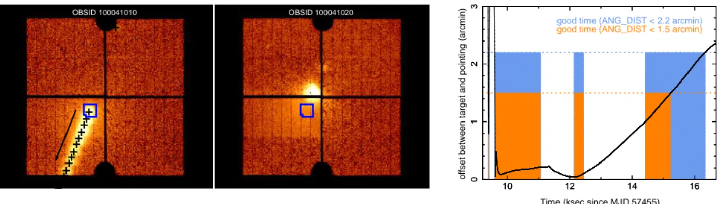
After the Perseus observations, Hitomi aimed at the SNR N132D for performance verification of the SXS and SXI using another line-rich source. The other detectors, the Hard X-ray Imager (HXI) and Soft Gamma-ray Detector (SGD), were not yet turned on. Unfortunately, the satellite attitude control sys-tem lost control about 30 minutes after the observation started due to problems in the star tracker system, as illustrated in fig-ure 1. Because of this, the SNR drifted out of the 3′
× 3′SXS FoV and remained out of view for the remainder of the observa-tion. Thanks to its larger FoV, the SXI was able to observe the source during the entire observation.
As this observation took place during the commissioning phase, several instrument settings were non-standard compared to expected science operation. First, the SXS gate valve was in the closed configuration to reduce the chance of molecu-lar contamination from spacecraft out-gassing. The gate valve had a ∼ 260µm thick Be window to allow observations while closed, but this absorbed almost all X-rays below ∼ 2 keV and reduced the effective area by ∼ 50% at higher energies (Eckart et al. 2016). Thus we limit our SXS analysis to the 2–10 keV regime. Second, while the SXS was close to thermal equilib-rium at this point in the commissioning phase (Fujimoto et al. 2016; Noda et al. 2016), no on-orbit, full-array energy scale (or gain) calibration had been performed with the filter-wheel cali-bration sources. The Modulated X-ray Source (MXS; de Vries et al. 2017) was also not available for contemporaneous gain measurement. A dedicated calibration pixel that was outside of the aperture and continuously illuminated by a collimated55Fe
source served as the only contemporaneous energy-scale refer-ence, and the time-dependent scaling required to correct its gain
was applied to each pixel in the array (Porter et al. 2016b). It was well known prior to launch that the time-dependent gain-correction function for this calibration pixel generally would not adequately correct the energy scale of the array pixels. In particular, the relationship between changes on the calibration pixel and on the array was not fixed, but rather depended on the temperatures of various shields and interfaces in the SXS dewar. Therefore, although the relative drift rates across the ar-ray were characterized during a later calibration with the filter-wheel55Fe source (Eckart et al. in prep.), changes in SXS
cry-ocooler settings between the N132D observation and that cali-bration limit the usefulness of that characterization.
In fact, the measured relative gain drift predicts a much larger energy-scale offset between the final two pointings of the Perseus Cluster than was actually observed. Using source-free SXS observations taken during the period with the same cry-ocooler settings as the N132D observation (2016 March 7-15) in order to circumvent this limitation, we measured the cen-ter of the Mn Kα instrumental line (Kilbourne et al. in prep.), and conclude that the SXS energy scale is shifted by at most +1 ± 0.5 eV at 5.9 keV (Eckart et al. in prep.). There are no sufficiently strong low-energy lines in the same data set, but extrapolating from Perseus Cluster observations, we estimate a gain shift of −2 ± 1 eV at 2 keV (Hitomi Collaboration, in prep. [Perseus cluster atomic data paper]). In the filter-wheel
55Fe data set, errors in the position of the Mn Kβ line ranged
from −0.6 to +0.2 eV across the array. Since this line is at 6.5 keV, less than 1 keV from the Mn Kα reference line, gain errors at other energies further from the reference may be sub-stantial. This is especially true in science data, for which drift of the energy scale can only be corrected via the data from the calibration pixel. To be conservative, we use a systematic gain error of ±2 eV at all energies in the analysis below.
We analyzed the cleaned event data of the final pipeline pro-cessing (Hitomi software version 6, CALDB version 7) with the standard screening for both SXS and SXI (Angelini et al. 2016), with one exception. To maximize the good SXS observ-ing time, we relaxed the requirement that eliminates data when the aimpoint is further than 1.′5 from the target position. Using a
maximum angular offset of 2.′2 ensures that at least 50% of the
SNR is still in the FoV, and it increases the good SXS exposure time from 2,610 s to 3,737 s (by 43%) and the total SXS counts in the 2–10 keV band from 198 to 233 (by 18%). Relaxing this criterion increased the counts in the FeXXVHeα band (de-fined in section 3.1) from 16 to 17, and in the SXVHeα band (defined in section 3.2) from 13 to 16. As we show in section 3, with the very low SXS background and very high spectral resolution, this small number of counts is sufficient to derive in-teresting constraints for the line centers. Some of the additional broad-band counts are from the region outside the N132D emis-sion peak, as shown in figure 2, so they are likely background
OBSID 100041010 OBSID 100041020 10 12 14 16 0 1 2 3 10 12 14 16 0 1 2 3
good time (ANG_DIST < 2.2 arcmin)
good time (ANG_DIST < 1.5 arcmin)
Time (ksec since MJD 57455)
offset between target and pointing (arcmin)
Fig. 1. (Left) SXI images in detector coordinates showing the two OBSIDs used in the SXI analysis. The blue square shows the SXS FoV. The arrow in the left panel shows the direction N132D drifted in the focal plane during that OBSID, with black crosses marking the source center in intervals of one hour. N132D was in the SXS FoV for only 3.7 ks of OBSID 100041010, and for none of OBSID 100041020. The remnant was still visible in SXI due to that detector’s larger FoV. (Right) Attitude of Hitomi during the first 7 ks of OBSID 100041010. The solid line shows ANG DIST, the angular distance in arcmin between the intended pointing and the actual pointing. Orange bins show the good time intervals of the default data filtering, which requires ANG DIST < 1.′5. Blue bins show the additional ∼ 43% of time added by relaxing this criterion to 2.′2. Blank times are excluded because of Earth occultation or South Atlantic Anomaly passage.
Fig. 2. Images of the SXS showing individual counts as a pixel on the sky. Blue boxes are counts included after relaxing the angular distance criterion. The red contours trace the Chandra emission, and the green circles show radii of 1.′5 and 2.′0 from the Chandra peak. The counts in Fe K (right) correspond well to the remnant extent, while some of the counts in the other bands are outside the bounds of the remnant.
counts. The extra counts in the lines are consistent with loca-tions in the remnant, also shown in figure 2; in particular, to the extent that we can infer locations from the ∼ 1′Hitomi PSF,
the S counts are found largely in the rim of the remnant, while the additional Fe K count (and all the Fe K counts) are concen-trated in the remnant center, consistent with what is seen with XMM-Newton (Behar et al. 2001).
We constructed an SXS source spectrum by extracting only GRADE Hp (high-resolution primary) events from the entire SXS field of view of OBSID 100041010, and created the re-distribution matrix file (RMF) with sxsrmf, using the medium size option. The ancillary response file (ARF) was generated with aharfgen, using a high-resolution Chandra image as input to the ray-tracing. A non-X-ray background (NXB) spectrum with the same sampling of magnetic cut-off rigidity as the ob-servation and with identical filtering as the source data (except for Earth elevation criteria) was extracted from the SXS archive NXB event file using sxsnxbgen. In the 2–10 keV band, we ex-pect 23.2 ± 0.6 NXB counts, about 10% of the observed count rate, and corresponding to ∼ 0.4 counts per spectral resolution element per 100 ks. In the narrow bands used for the analysis
that follows, the NXB count rate is less than 5% of the observed rate as the SXS NXB is almost featureless and nearly constant over the energy range (Eckart et al. in prep.).
For the SXI, both OBSIDs 100041010 and 100041020 were used, although for the former we enforced the requirement that the aimpoint be within 1.′5 of the target to eliminate
complica-tions in constructing a response for a source moving across the FoV. For OBSID 100041020, we used only times when the at-titude was stable, although the source was not at the expected aimpoint and was partially obstructed by the chip gaps (see fig-ure 1). The final good exposfig-ure time for the SXI was 35.4 ks.
An SXI spectrum was extracted from a 2.′5 radius circle with
center (RA,Dec) = (5h25m02.s2,−69◦38′39′′). The NXB
spec-trum was produced with sxinxbgen, using the entire SXI FoV excluding the source in order to increase the statistics. To prop-erly scale the NXB normalization between the full FoV and source region, the instrumental lines of Au Lα and Lβ were used, producing a scaling factor of 0.0070. RMF and ARF files were generated with and sxirmf and aharfgen, respectively.
3 SXS Spectral Analysis
With only 233 counts, the SXS spectrum is dominated by Poisson low-count statistics. In addition, with the SXS gate valve closed, the bright emission lines of C, O, Ne, and Mg be-low 2 keV are not observable. However, three emission features are easily seen in the full-band spectrum shown in figure 3, the Heα transition features of He-like S (∼ 2.45 keV), Ar (∼ 3.1 keV), and Fe (∼ 6.7 keV). These lines are clearly detected in previous observations dating back to BeppoSAX (Favata et al. 1997), although the combination of an extended source and lower sensitivity at these energies complicates their measure-ment by X-ray grating instrumeasure-ments like Chandra/HETGS and XMM-Newton/RGS. From narrow bands centered on each
ex-10 2 5 0 5 10 S XV K Ar XVII K Fe XXV K Energy (keV) Counts
Fig. 3. Full-band SXS spectrum of N132D, showing counts with Poisson er-rorbars from Gehrels (1986). The orange points show the total estimated background, which has not been subtracted. Both spectra are binned to 16 eV for display purposes.
pected line centroid, the total number of counts and estimated NXB counts are 16 total (0.30 ± 0.07 NXB) counts for SXV Heα; 14 total (0.28 ± 0.06 NXB) counts for ArXVIIHeα; and 17 total (0.8 ± 0.1 NXB) counts for FeXXVHeα. The signal-to-noise of these features and the underlying continuum is in-sufficient to obtain useful constraints on the metal abundance, temperature, or velocity broadening of the emitting plasma. However, as we show below, given a reasonable spectral model from other sources, the exquisite spectral resolution of SXS al-lows us to measure the line centers and thus the average line-of-sight Doppler velocity of two of these components, S and Fe.
All spectral fitting described below was performed with XSPEC v12.9.1d (Arnaud 1996), using atomic and non-equilibrium ionization (NEI) emissivity data from AtomDB v3.0.8 (Foster et al. 2012), and abundance ratios from Anders & Grevesse (1989). In each restricted fitting region, we allowed only the line-of-sight velocity and normalization of the appro-priate thermal component (described below) to vary in the ini-tial fit. While we include the cosmic X-ray background (CXB), it is negligible; a reasonable model for the 2–10 keV contribu-tion of the CXB power law component with Γ = 1.4, S(2–10 keV) = 5.4 × 10⁻¹⁵erg cm−2s−1arcmin−2(e.g., Ueda et al.
1999; Bautz et al. 2009) predicts a mean of 1.5 CXB counts across the entire band and less than 0.1 CXB counts in any of the narrow spectral analysis bands. This is less than 1% of the de-tected counts. Galactic foreground emission is negligible above 2 keV toward this direction (l = 280◦,b = −32.◦8).
3.1 Iron Region Spectral Analysis
Fe K emission in N132D has been explored previously (Favata et al. 1997; Behar et al. 2001; Xiao & Chen 2008; Yamaguchi et al. 2014), with the conclusion that this feature is dominated
by FeXXVHeα emission. The XMM-Newton/EPIC observa-tions are successfully fit above 2.5 keV with a two-temperature-component model withkT = 0.89 and 6.2 keV (Behar et al. 2001). The cooler component produces the strong soft emission lines seen with XMM-Newton/RGS, and the hotter component explains the Fe K emission. In particular, Behar et al. (2001) emphasize the lack of a temperature component at ∼ 1.5 keV to explain the lack of observed L-shell emission from Li-, Be-, and B-like Fe in the XMM-Newton spectrum. A recent study using 240 ks of Suzaku data combined with a 60 ks NuSTAR observa-tion (Bamba et al. 2017) has produced a two-component broad-band spectral model of N132D with a similar cool temperature (kT ≈ 0.8 keV) but that interprets the Fe K emission arising pri-marily from an over-ionized, recombining plasma component withkTe= 1.5 keV, kTinit> 20 keV, and relaxation timescale
net ≈ 10
12s cm−3. Crucially, the Suzaku data show a clear
detection of H-like Fe Lyα emission, indicating that an under-ionized (ionizing) plasma is unlikely to contribute significantly to the emission at these energies, and thus much of the otherwise unresolved Fe K emission is likely due to He-like Fe rather than lower ionization states.
These previous observations provide confidence that we know where the line centroid should be for the Fe K complex, and can cleanly measure the line-of-sight velocity. However, we emphasize that this is one possible interpretation of a plasma with strong FeXXVHeα and measurable FeXXVILyα emis-sion. A more complicated temperature structure, such as from multiple unassociated, spatially unresolved components, could produce a very different complex of lines in this spectral re-gion. We address this possibility further in section 5. To ease comparison to current work, we adopt the model from Bamba et al. (2017) as a baseline model, shown in figure 4 and table 3.1.
The FeXXVHeα complex, shown in figure 5, was fit within the energy range 6.45–6.80 keV. This range includes sufficient width to constrain the continuum and measure velocity shifts up to ∼ 7000 km s−1, but avoids contamination from a
possi-ble 6.4 keV Fe K line and any H-like Fe features. It is clear from figure 4 that in this very clean fitting region the model is dominated by emission from the recombining plasma com-ponent by at least a factor of 100 over the cooler collisional ionization equilibrium (CIE) component. Therefore, while we included the entire model with all components for the Fe region fit, we only allowed parameters related to the NEI component to vary. To allow for differences in the observed flux due to the smaller SXS FoV and attitude drift, we fixed the ratio of the CIE to NEI component normalizations to that derived by Bamba et al. (2017), and allowed the NEI flux to vary along with the line-of-sight velocity. The CIE component was mod-eled by a variable-abundance vapec model in XSPEC, while the NEI component was modeled by a variable-abundance
recom-2.3 2.4 2.5 2.6 0 5×10 −3 0.01 0.015 Si XIV S XV Si XIV NEI CIE 2.3 2.4 2.5 2.6 0 5×10 −3 0.01 0.015 6.20 6.4 6.6 6.8 7 10 −4 2×10 −4 3×10 −4 Fe I Fe XXV Fe XXVI CIE NEI 6.20 6.4 6.6 6.8 7 10 −4 2×10 −4 3×10 −4 Energy (keV)
Photon flux density (cm
−2
s
−1
keV
−1)
Fig. 4. N132D model spectrum, with contributions from individual compo-nents shown along with the total spectrum (black). All compocompo-nents are plot-ted with zero velocity and no line broadening. In the FeXXVHeα band (left), the NEI component (blue) dominates by a factor of ∼ 100 over the CIE com-ponent (orange). In the SXVHeα band (right), the CIE component is ∼ 10 times brighter than all other components. The gray shading indicates the bands used for spectral analysis; the S region is chosen to exclude contribu-tions from SiXIV, while the Fe region is chosen to exclude the bright neutral Fe K line (yellow) and the FeXXVIfeature, but include possible contributions from lower ionization states of Fe near 6.5 keV.
bining plasma model, vrnei. We included a single Gaussian broadening parameter to allow for thermal and turbulent broad-ening as well as unresolved bulk motion.
Parameter estimation was performed in two ways. First, maximum likelihood estimation was done by minimizing the fit statistic, using cstat in XSPEC, a modified Cash (1979) statistic. With the broadening width fixed at zero, this fitting revealed a highly non-monotonic parameter space for the ve-locity (see figure 6), likely due to the combination of low-count Poisson statistics in the data and discrete spectral features in the model. The best-fit velocity of vhelio = 1440km s−1 is
significantly larger than the value of the local LMC ISM sur-rounding N132D,vhelio,LMC= 275 ± 4km s−1(Vogt & Dopita
2011). Allowing a free broadening width eliminated this non-monotonicity (see figure 7), resulting in a best-fitvhelio= 1140
km s−1and broadening ofσ = 510 km s−1
.
Second, to fully explore parameter space, we performed Markov chain Monte Carlo (MCMC) simulations within XSPEC using Bayesian inference. These simulations were run with and without velocity broadening, using both a flat (uni-form) prior distribution and a Gaussian prior distribution for the broadening width. The width of the Gaussian prior distribution was chosen to reflect current upper limits on the velocity broad-ening. In particular, observations with CCD-based X-ray obser-vatories such as Suzaku (e.g. Bamba et al. 2017) have not found measurable broadening. The typical spectral resolution of such instruments near 6 keV is ∼ 150–180 eV FWHM, depending on the epoch of observation, with a typical 1-σ calibration
uncer-tainty of 5%2. This calibration uncertainty can be thought of as an upper limit on the detectable line broadening velocity. Since the broadening is a convolution, this extra velocity component adds in quadrature with the instrumental width. We find that a 5% increase on the 150–180 eV FWHM instrumental width is equivalent to an extra broadening component with FWHM of 48–58 eV, orσ = 900–1100 km s−1
in the center of our fit-ting band. We therefore adopted 1000 km s−1as a natural 1-σ
width to use for the Gaussian prior distribution. We performed MCMC simulations using both the flat, uninformative prior and the weakly informative Gaussian prior.
The MCMC results are consistent with the local cstat min-ima in velocity parameter space for fits with and without broad-ening, as shown by the MCMC posterior probability distribu-tions in figures 6 and 7. In particular, the complicated velocity posterior distribution shows up clearly in the MCMC runs with-out broadening, but with the most likely value (highest mode)
nearvhelio= 800km s−1instead of 1400 km s−1as found in
the cstat minimization. The MCMC chain steps shown in fig-ure 6 (right) indicate that the simulation is well-behaved and samples the posterior distribution adequately despite the multi-modal structure. The runs with broadening result in Gaussian posterior distributions with peak near 1000 km s−1. Using ei-ther a Gaussian or Cauchy form for the chain proposal distribu-tion produced the same results.
We used these posterior distributions to obtain central cred-ible intervals onvhelio. For the fit with no broadening, a
sin-gle interval is uninformative due to the complicated structure. We obtain a 68% credible interval of 730–1460 km s−1, 90%
interval of 440–1540 km s−1, and 95% interval of 160–1620
km s−1. A line-of-sight velocity consistent withv
helio,LMCis
ruled out at 93% confidence under this model. With broaden-ing, a single credible interval is sufficient to characterize the Gaussian-shaped distribution, and we find 90% credible inter-vals of 330–1780 km s−1for broadening with a Gaussian prior distribution, and 0–2090 km s−1 for a flat prior. The
conser-vative gain uncertainty of ± 2 eV (see section 2) produces a systematic uncertainty of ± 90 km s−1, well within the
statisti-cal uncertainty. It is apparent that imposing an flat, uninforma-tive prior on the broadening width distribution allows unrealis-tic values exceedingσ = 3000 km s−1with a broad tail to very
high values. This greatly exceeds the thermal width of an Fe emission feature at 2 keV (σ ∼ 50 km s−1), and requires either
extreme turbulence or very large bulk motions. If we adopt the results with the Gaussian prior, which has sufficient width to allow a blueshifted and redshifted component separated by up to ∼ 2000 km s−1, a mean line-of-sight velocity consistent with
vhelio,LMCis ruled out at 91% confidence under this model. The
model parameters are listed in table 3.1.
2See Table 3.2 and Figure 7.11 of the Suzaku Technical Description, ftp://legacy.gsfc.nasa.gov/suzaku/nra info/suzaku td xisfinal.pdf.
6.5 6.6 6.7 0 2 4 6 6.5 6.6 6.7 0 2 4 6 Fe XXV K model BG Energy (keV) Counts 2.42 2.44 2.46 0 2 4 6 2.42 2.44 2.46 0 2 4 6 S XV K Energy (keV) Counts
Fig. 5. SXS spectra of the (left) FeXXVHeα and (right) SXVHeα fitting regions. The data points are detected SXS counts with Poisson error bars from Gehrels (1986). In both panels, the blue shaded region shows the best-fit model, and the black shaded region, barely visible, shows the estimated total background. In the left panel, the dotted line shows the model with velocity fixed at vhelio,LMC=275 km s−1. The Fe spectrum is binned to 16 eV and S binned to 4 eV for display purposes.
Table 1. Results of SXS Spectral Fitting.∗
Model Parameter FeXXVfit SXVfit
no broadening with broadening† no broadening with broadening† N132D CIE plasma (vapec)
kT (keV) . . . 0.7 . . . . ZSi(solar) . . . 0.6 . . . . ZS(solar) . . . 0.9 . . . . ZFe(solar) . . . 0.4 . . . . vhelio(km s−1) . . . 0 . . . 210+370−380 520 +770 −620 σ (km s−1) . . . 0 . . . . 0 520+780 −340 flux, 2–10 keV‡ . . . 8.8. . . 5.6+2.9−1.9 5.5 +3.1 −1.8
flux, fitting band‡ . . . 0.006 . . . . 1.3+0.4
−0.2 1.3
+0.4 −0.2
N132D NEI plasma (vrnei)
kT (keV) . . . 1.5 . . . . kTinit(keV) . . . 80 . . . . net (10 12s cm−3) . . . 0.9 . . . . ZSi(solar) . . . 0.4 . . . . ZS(solar) . . . 0.4 . . . . ZFe(solar) . . . 0.5 . . . . vhelio(km s−1) 1440+100−1000 1140 +640 −810 1440 1140 σ (km s−1) 0 510+1060 −330 0 510 flux, 2–10 keV‡ 9.5+4.5 −3.0 9.7 +4.2 −3.2 6.1 6.2
flux, fitting band‡ 0.48+0.25−0.16 0.49 +0.24
−0.16 0.34 0.34
CXB power law
Γ . . . 1.54 . . . . flux, 2–10 keV‡ . . . 0.040 . . . .
flux, fitting band‡ . . . 0.0016 . . . . . . . 0.0006 . . . .
spectral fitting band . . . 6.45–6.80 keV . . . 2.40–2.48 keV . . . . C-stat / d.o.f. 107.9 / 696 106.5 / 695 61.0 / 157 59.1 / 156
goodness-of-fit (KS)§ 24% 20% 62% 31%
goodness-of-fit (CvM)§ 35% 21% 62% 46%
∗Unless noted otherwise, values without quoted uncertainties are fixed. Uncertainties are 90% confidence limits. †Results with broadening are from inference with a Gaussian prior with σ = 1000 km s−1.
‡Flux is given in units of 10−12erg cm−2s−1. The ratio of the vapec and vrnei component normalizations was fixed to that in Bamba et al. (2017).
§“Goodness-of-fit” is the percentage of simulated observations with lower fit statistic than the real data, as described in section 3.1.
0 500 1000 1500 2000 0 0.02 0.04 0.06 0.08 −90% +90% LMC Fe no broadening 0 500 1000 1500 2000 0 0.02 0.04 0.06 0.08 110 115 120 125 130 vhelio (km s−1)
vrnei model normalization
c−stat 0 50000 100000 150000 0 1000 2000 0 50000 100000 150000 MCMC chain step vhelio (km s −1 )
Fig. 6. (left) Posterior probability distributions of the vrnei model normalization (orange) and velocity (blue) from the Fe K region fitting without broadening, calculated from the MCMC analysis as described in the text. Points show sample MCMC chain steps, indicating that there is no correlation between the two parameters. The black line shows the cstat value from fit statistic minimization, as a function of best-fit velocity. One peak of the MCMC velocity distribution coincides with the best-fit velocity distribution, and other local peaks coincide with local cstat minima, indicating both maximum likelihood methods produce the same result. The dotted lines delineate the central 90% credible interval and note the local LMC velocity. (right) MCMC chain values for the Fe K velocity plotted against chain step, showing that the long-term variations of each chain are well-behaved and the posterior distribution is well-sampled. Vertical lines differentiate the eight individual 20,000-step simulation chains. Steps within chains are in time order with one out of every ten steps shown for clarity.
0 500 1000 1500 2000 2500 0 2000 4000 −90% +90% LMC Fe flat prior on broadening 0 500 1000 1500 2000 2500 0 2000 4000 108 110 112 114 vhelio (km s−1) line broadening σ (km s −1) c−stat 0 500 1000 1500 2000 2500 0 2000 4000 −90% +90% LMC Fe Gaussian prior on broadening 0 500 1000 1500 2000 2500 0 2000 4000 108 110 112 114 vhelio (km s−1) line broadening σ (km s −1) c−stat
Fig. 7. Posterior probability distributions of the vrnei model broadening width (orange) and velocity (blue) from the Fe K region fitting including line broadening. Notations are the same as in figure 6. The left panel shows results with flat prior on the line width, while the right panel shows results imposing a Gaussian prior with 1-σ width of 1000 km s−1. Both velocity distributions trace the cstat minimization well. The flat prior produces a broader posterior distribution.
The measured photon flux in the fitting band, 4.6+2.3
−1.4×
10−5 ph cm−2 s−1, is more than a factor of two higher than
previous estimates of the Fe Kα line flux, e.g. 1.83 ± 0.17 × 10⁻⁵ ph cm−2 s−1 (Yamaguchi et al. 2014; errors are 90%).
This is likely due to a combination of the Hitomi attitude uncer-tainty and the use of a broad-band X-ray image to produce the response files. While much of this broad-band X-ray emission is found in a shell with diameter ∼ 2′, the Fe Kα emission appears
centrally concentrated (e.g., Behar et al. 2001). Using the more spatially extended broad-band image produces a lower response as some of the PSF-broadened flux falls outside of the 3′× 3′
SXS FOV, thereby increasing the inferred model flux for a given count rate. Our inclusion of data with large pointing offset of up to 2.2′ and the large attitude drift undoubtedly exacerbate
this effect. For this reason, the flux calibration is so uncertain that a flat, uninformative prior is a good representation of our knowledge of the SXS effective area for this observation.
Once the minimum fit statistic and parameter distribution function were determined, we explored the effects of adjust-ing other vrnei parameters within a reasonable range of uncer-tainty. In addition, we ran fits testing plasma models with higher over-ionization (settingnet to a small value), under-ionization
(an ionizing plasma, settingkTinit< kT ), and collisional
ioniza-tion equilibrium (CIE, settingkTinit=kT ). The fit statistic was
consistent in all cases, indicating that we cannot distinguish be-tween various ionization states with the Hitomi/SXS data alone. In all cases, neither the best-fit velocity nor its posterior distribu-tion from the MCMC analysis changed appreciably, indicating that our results are insensitive to the exact emission model used so long as it is not highly complex.
Neither the XSPEC cstat statistic nor the MCMC analysis provides an estimate of the goodness of fit. We used two tests available in XSPEC, Kolmogorov-Smirnov (KS) and Cramer-von Mises (CvM), both of which treat the observed and model spectra as empirical distribution functions and compute a sta-tistical difference between the two. Drawing parameter values for velocity, normalization, and broadening width from the full posterior distributions, we performed 1000 simulations of the observed 3.7 ksec spectrum for the fits with and without broad-ening. These simulated spectra were then fit with the model, and the resulting KS and CvM test statistics were compared with the values from the original fits. For the fit without broadening, 24% of the realizations produced a smaller KS statistic than the best fit, and 35% produced a smaller CvM statistic. For the fits with broadening, the fractions were 20% for KS and 21% for CvM. We can only say that our best-fit models are not statisti-cally inconsistent with the data.
Since this asymmetric velocity structure is unexpected, we constrained a potential blue-shifted emission feature by adding a second vrnei component with identical model parameters. The velocity of the first component was fixed to the best-fit
value of 1140 km s−1, while that of the new component was
fixed to −590 km s−1, to force symmetry about v
helio,LMC.
The vrnei normalizations, initially equal, were allowed to vary independently. We find that a blue-shifted feature is allowed at up to 30% of the flux of the redshifted component, with a similar fit statistic and goodness-of-fit measure. Varying the blueshift within a reasonable range did not improve the fit or change the upper limit to its flux. The best-fit broadening width (σ ∼ 500 km s−1
or FWHM ∼ 1200 km s−1) allows some blueshifted component, but the emission-weighted mean veloc-ity is not centered on the LMC velocveloc-ity. We conclude that the bulk of the He-like-iron-bearing material is receding asymmet-rically, at a velocity ∼ 800 km s−1with respect to the swept-up
ISM surrounding N132D.
3.2 Sulfur Region Spectral Analysis
Spectral fitting of the SXVHeα line proceeded in a similar man-ner to the Fe K region. We restricted the eman-nergy range to 2.40– 2.48 keV, leaving 16 total counts of which 0.30 ± 0.07 (∼ 2%) are estimated to be from the NXB. Consistent with other re-cent work, we interpret the SXV Heα emission to arise pre-dominantly from a CIE plasma withkT ∼ 1 keV (Behar et al. 2001; Borkowski et al. 2007; Xiao & Chen 2008). In our base-line model, the CIE component dominates the NEI emission by a factor of ∼ 5–10 in this region. Thus we allowed some small contamination from the high-redshift NEI emission by freez-ing the velocity and broadenfreez-ing of the vrnei component to the best-fit values, and fixed the ratio of the vapec to vrnei normal-izations to that found by Bamba et al. (2017). Only the velocity and normalization of the CIE vapec component were allowed to vary in the initial fit, but as with the Fe fit, we included broad-ening with similar priors to explore the effect on the derived velocity. The S region spectrum and model are shown in figure 5, posterior probability distributions are shown in figure 8, and best-fit parameters are given in table 3.1.
Using the cstat maximum likelihood estimator, we obtain a best-fit line-of-sight velocity ofvhelio= 210km s−1with
broad-ening fixed at zero. Allowing a single broadbroad-ening component results invhelio= 520km s−1withσ = 520 km s−1. As with
the Fe fitting, the posterior distributions in figure 8 are consid-erably wider when broadening is included, with 90% credible intervals on vhelio of −170 to +580 km s−1 with no
broad-ening and −100 to +1290 km s−1 with a Gaussian prior on
broadening withσ = 1000 km s−1. Unlike for Fe, the
veloc-ity of the S component is completely unconstrained with a flat broadening prior. Our adopted SXS gain uncertainty of ± 2 eV (245 km s−1; see section 2) is again well within this
statisti-cal uncertainty, which itself is consistent with the lostatisti-cal LMC velocity of 275 km s−1.
−500 0 500 1000 1500 2000 0 0.05 0.1 0.15 0.2 −90% +90% LMC S no broadening −500 0 500 1000 1500 2000 0 0.05 0.1 0.15 0.2 65 70 75 80 vhelio (km s −1)
vapec model normalization
c−stat −500 0 500 1000 1500 2000 0 500 1000 1500 2000 −90% +90% LMC S Gaussian prior on broadening −500 0 500 1000 1500 2000 0 500 1000 1500 2000 60 65 70 vhelio (km s −1) line broadening σ (km s −1) c−stat
Fig. 8. Posterior probability distributions for the S region fit. In the left panel, vapec model broadening is fixed at zero, and the posterior model normalization is shown in orange. In the right panel, a Gaussian prior with width σ = 1000 km s−1is imposed on the broadening, and the posterior broadening distribution is shown in orange. The velocity posterior distribution is shown in blue in both panels. Other notations are the same as in figure 6. Both velocity posterior distributions are Gaussian in shape and trace the cstat minimization well. The model with broadening produces a broader distribution shifted to higher velocity, but still consistent with the local LMC velocity.
CIE component andkT , kTinit, net, and σ of the
recombin-ing plasma component to vary over a broad range as in the Fe region fitting described in the previous section. The best-fit ve-locity and credible intervals did not change. We performed the same goodness-of-fit tests to the S region fits as the Fe region fits, finding that 30–60% of the simulated datasets produced a smaller test statistic. The model is thus consistent with the data, and we conclude that the He-like-sulfur-bearing gas is consis-tent with being at rest relative to the local LMC ISM, if we assume that line broadening is small.
3.3 Argon Region Spectral Analysis
Spectral fitting of the ArXVIIHeα line is complicated by both the low number of total counts (14) and the estimated contri-butions from both CIE and NEI components. In fact, the Ar abundance is not constrained in either component, leading to a degeneracy between the normalization and abundance in each component and further difficulty fitting different velocities. As a simple test, we fixed the vapec and vrnei normalizations to the Bamba et al. (2017) values, fixed the Ar abundance to solar for both components, and fit a single line-of-sight velocity and normalization. The best-fit velocity isvhelio= 2400 km s−1,
with a 90% credible interval of 570–5900 km s−1. This is consistent with both velocity ranges of FeXXV and SXV. If the velocities are tied at the offset to the best-fit values so thatvvrnei = vvapec + 1200 km s−1, the fit statistic is only
slightly worse (cstat = 81.2 vs. 80.8), and the best-fit values
arevhelio= 1800km s−1 for the vrnei component and 600
km s−1for the vapec, with similar uncertainties. Given the
un-certainties in the model, we can only conclude that the ArXVII fit is consistent with the Fe and S line results.
4 SXI Spectral Analysis
For the following analysis, the same version of XSPEC, AtomDB, NEI emissivity data, and abundance tables were used as in the analysis of the SXS spectrum (see section 3). The NXB-subtracted spectrum is shown in figure 9. In the N132D observation, the event and split thresholds are 600 eV and 30 eV, respectively. Since charge from a detected X-rays may be split among multiple CCD pixels, the quantum efficiency (QE) can be affected by split events well above the event threshold. Given the limited amount of calibration information available in these early observations, we conservatively exclude the energy band below 2 keV in this study.
We detect emission lines at 2.456 ± 0.010 keV and 6.68 ± 0.04 keV, which correspond to the same Heα lines of S and Fe detected in SXS, respectively. The SXI is affected by light leak when the satellite is in daylight, which can result in an observed line center shift (Nakajima et al. in prep.). We investigated the line center shift in the N132D data, and confirmed that daylight illumination of the spacecraft has no effect. The SXVHeα line center is fully consistent with the centroid of the line complex measured with SXS (see figure 5). The FeXXVHeα line center is marginally consistent with SXS within the uncertainty (see figure 5), and likely includes some unresolved contribution from FeXXVILyα at ∼ 7 keV (see figure 4).
Following the SXS analysis, we adopted a spectral model with two thin-thermal plasmas, a low-temperature vapec and high-temperature vrnei. From the model of Bamba et al. (2017), we also include a 6.4 keV neutral Fe K line, a non-thermal component, and the CXB. In the SXI analysis, the nor-malizations of the two plasmas are set to be free and all the other thermal parameters are fixed to those of Bamba et al. (2017). The normalization of the FeIK line was tied to that
10 1 0 −5 1 0 −4 1 0 −3 0 .0 1 0 .1 1 1 0 C o u n ts s −1 ke V −1 Energy (keV) 5 1 2
Fig. 9. SXI spectrum of N132D. Black data points show the full spectrum, red show the scaled NXB spectrum, and blue show the NXB-subtracted spec-trum. Emission over the background is clearly seen above 10 keV.
of the vrnei component using the ratio of normalizations from Bamba et al. (2017). A power-law model was added for the possible non-thermal component, with both photon-index Γ and normalization allowed to vary. For the CXB, another power-law model with fixed parameters of Γ = 1.4 and surface brightness 5.4 × 10⁻¹⁵
erg cm−2s−1arcmin−2in the 2–10 keV band was used (Ueda et al. 1999; Bautz et al. 2009). This CXB intensity is expected from observations with previous X-ray imaging in-struments with similar PSF, and thus similar confusion limits. Since we are in the high-counts regime with at least 30 counts per spectral bin in the total (unsubtracted) source spectrum and high statistics in the NXB spectrum, we expect the background-subtracted spectral bins to be Gaussian distributed and useχ2
minimization. We obtain χ2/d.o.f.= 234/243 and an
accept-able fit at the 90% confidence level. The best-fit model with individual components is shown in figure 10. To check for po-tential bias in the use ofχ2 statistics, we perform the fit again
excluding the poorest statistical region above 9 keV, and obtain similar results.
The lower and higher temperature plasmas produce the ma-jority of the Heα lines of S and Fe, respectively, consistent with the result of the previous study (see also figure 4). The best-fit vapec normalization was 0.92 ± 0.03 of the value from Bamba et al. (2017), while the vrnei was 0.86 ± 0.10 of their best-fit value. The model best-fitting results in a non-thermal compo-nent with flux 1.3 ± 1.1 × 10⁻¹³erg cm−2s−1in the 2–10 keV
band. If we assume this non-thermal component exists, the fit constrains the photon index to be Γ< 3.0. With the SXI data in hand, we are unable to say conclusively that the non-thermal component is required, only that it is consistent with the ob-served spectrum. 10−4 10−3 0.01 0.1 Count s s −1 ke V −1 10 2 5 −4 −2 0 2 4 (da ta −m ode l)/ error Energy (keV)
Fig. 10. SXI spectrum of N132D fitted with the model discussed in the text, with individual components shown. Two thin-thermal plasma components are shown with orange (vapec) and red (vrnei) lines. The 6.4 keV Fe K line is shown in blue, the CXB power law component in green, and the marginally detected non-thermal component in magenta.
5 Discussion
We have revealed a significant redshift of the emission lines of He-like Fe, constraining the line-of-sight velocity to be ∼1100 km s−1, or ∼ 800 km s−1 faster than the local LMC ISM. The emission of SXVHeα, on the other hand, shows a ve-locity consistent with the radial veve-locity of the LMC ISM, albeit with large uncertainty, especially when broadening is included in the model. These results suggest different origins of the Fe and S emission: the former is dominated by the fast-moving ejecta and the latter by the swept-up ISM. This interpretation is consistent with the previous work by XMM-Newton, which revealed that the Fe emission has a centrally-filled morphology and the S emission is found along the outer shell (Behar et al. 2001).
This interpretation hinges on our assumed underlying emis-sion model. Previous results from XMM-Newton (Behar et al. 2001) and the detection of an FeXXVILyα line in the Suzaku spectrum (Bamba et al. 2017) suggest minor contamination from lower-energy, lower-ionization states of Fe. It is possible that the H-like Fe emission arises from a much hotter plasma that does not produce He-like emission, and the Fe K com-plex in question is produced by lower-temperature plasma un-resolved by both the Suzaku and Hitomi PSF. Although L-shell lines of lower-ionization Fe were not detected by (Behar et al. 2001), it is further possible that the L-shell energy band is domi-nated by the low temperature swept-up ISM component, hinder-ing detection of faint ejecta lines. We are unable to conclusively demonstrate the validity of our assumptions with existing X-ray data, and we stress that the discussion that follows assumes the Fe K emission is dominated by He-like Fe.
The best-fit broadening widths for both Fe K and S K, σ ∼ 500 km s−1
, greatly exceed thermal broadening at these temperatures. It is unclear whether the constraints on