Archetypes for histogram-valued data

(1)

Archetypal analysis for

histogram-valued data

An application to Italian school system in a

benchmarking perspective

Francesco Santelli

A thesis presented for the PhD in

Social Sciences and Statistics

Department Of Social Sciences

University Federico II of Naples

XXXI Ciclo

Supervisors:

Prof. Francesco Palumbo

Prof. Enrica Morlicchio

(2)

(3)

Introduction

The present work set itself in the recent debate about the paradigm shift in statistical learning. Such new paradim is, in the last years, developed mainly from the birth of Big Data. Big Data re-framed the way in which scientific research and the constitution of knowledge itself is performed, changing also the nature of the information categorization process (Boyd and Crawford,

2012). According to recent estimates, data scientists claim that the volume

of data would roughly double every two years thus reaching the 40 zettabytes (ZB) point by year 2020, considering that a zettabyte is a unit of measure, that amounts to one sextillion of bytes, or equivalently to one trillion of gy-gabytes, used in digital information system. Including in such estimate also the Internet of things (IoT) impact, it is likely that the data amount will reach 44 ZB by 2020. Big Data is not simply denoted by volume, but also from the variety and the complex nature of such data. The three defining characteristics of Big Data, as a matter of fact, are often assumed to be the three V : volume (the data growth and the constant increase of the run rates), variety (data come now from various and heterogeneous sources, and assume several natures), and velocity (the source speed of data flows is increased to

the point that real-time data are available) (Zikopoulos, Eaton, et al.,2011).

If taking under consideration only the amount of data, a particularly wide dataset made up by simple data points, can be considered as well as a Big Data case. More interesting, and at the same time more challenging, is the recent and common context in which data are retrieved from sources that are specifically suited for data with a more complex structure. Methodologi-cal and techniMethodologi-cal difficulties are a common problem in using statistiMethodologi-cal tools when facing increasing complexity in data. To give some examples, data from most used Social Networks (Facebook, Twitter, Instagram and so on) present various types of nature and attributes: associated with each post, there is the text contained in the post itself, the author, the hashtags, the date and the hour related to the post, the geographical location of the author, and even pictures or videos are allowed to be included in the posted content. Conceiving statistical tools able to properly analyze and interpret data so

(6)

complex and heterogenous, is a tough task. But the information potentially included in that composite data is often large enough to be advantageous, in terms of statistical learning, to design and to develop techniques adequate for Big, and complex, Data. For these reasons a recurring theme associated to the new paradigm is Big Data opportunities (Labrinidis and Jagadish,

2012): more data are constantly available, and these kind of data have not

been easily analyzed before, opening a wide space of research and innovation ahead. This leads to propose new methods for the treatment of this type of data. The core of the contribution of this thesis goes to such direction. Several domains have been deeply transformed by the arrival of Big Data, and some of them, like social network platforms (Facebook, Twitter, Insta-gram) could be seen as the perfect workshops in which new data structures are developed. Other domains, like Business Analytics (BA) or Information Technology (IT), have obtained great advantage from the wide use of Big Data. For some other fields, on the other hand, the connection with Big Data issues seems to be less obvious and less expected. With respect to such assertion, among more unexpected domains, it comes out as a partic-ularly interesting case the Big Data radical shift in education (D. M. West,

2012). The onset of Big Data has affected both the pupils’ learning

pro-cess itself and the evaluation propro-cess of the educational system. For the former, many of the typical traditional tests provide just little immediate feedback to students, whom often fail to take full advantage of digital re-sources, so the improvement of the learning process is not as good as it could be. For the latter, most common way to evaluate school system is to assess pupils’ skills and performances for what concerns several domains; tra-ditional school evaluation can suffer from several limitations if disregarding Big Data opportunities. In the following, the focus will be on this particular aspect. At International level, the Programme for International Students

As-sessment (OECD-PISA),https://www.oecd.org/pisa/, is the organization

that analyses, in a comparative fashion, pupil’s skills in many Countries. In Italy, the school system evaluation is responsibility of the Istituto nazionale per la valutazione del sistema educativo di istruzione e di formazione

(IN-VALSI), http://www.invalsi.it/invalsi/index.php. These, and other

similar organizations, are able to gather a huge amount of information and data of different nature; most of the time, in a trade-off between complexity and analysis capability, the choice is to analyze data reduced to a simpler form. For example, several tests related to the same domain are reduced to their mean values for more advanced analysis, and the same happens in comparing school performances, losing so the internal variation of the phe-nomena. It is clear, therefore, that complexity is an opportunity but also a threat. Consistently, most of the statistical learning techniques used in this

(7)

context are aimed to reduce such complexity, finding salient units and/or clusters of units that can be properly described.

In the wide set of unsupervised statistical learning techniques, a specific role

is played by Archetypal Analysis (Cutler and Breiman, 1994). Archetypes

result as very useful salient units especially in account of their properties and location. They are extreme units, belonging to the convex hull of data cloud, defined as a linear combination of data units, meanwhile each data unit can be expressed as a linear combination of the identified archetypes. Therefore, they act as well separated units with extreme/peculiar behavior, suited for benchmarking purpose, as already proposed in (Porzio, Ragozini,

and Vistocco, 2006, 2008). This techinque have been used as a statistical

tool to achieve a benchmarking analysi,s in a quantitative internal

perspec-tive (Kelly, 2004; Smith, 1990), given that the aim, in the school system

assessment, is to find excellence standards and worst performances in a pub-lic sector. Archetypes have been already proposed and discussed for complex data, especially in Symbolic Data Analysis framework (SDA) (Billard and

Diday, 2006). Within this approach, the symbolic data table is an

aggrega-tion of simple points into hypercubes (broadly defined). This more complex data-matrix structure leads to define the intent as the set of characteristic descriptions, in the symbolic object, that defines a concept. Given the intent, the extent is the set of units in the data belonging to the concept accord-ing to the description (set of characteristics) and with respect to a rule of association. For this reason, in SDA, the core of the analysis is on the unit of second level (categories, classes or concepts) where units of the first level are aggregated into units of higher level. So, for example, based on given characterisics that are the intent, birds (individual units) can be grouped, using extent association, in species of birds (second level units). This ap-proach allows to retain much more information from original data, allowing for complex unit to present an internal variation and structure. Several on-tologies have been proposed for Symbolic Data (Noirhomme-Fraiture and

Brito,2011), and within this classification the focus will be, in this context,

on Histogram Symbolic Object, and on the relationship between Histogram-valued data and Interval-Histogram-valued data. In such SDA perspective, the proposed methodological approach refers to statistical learning techniques. The aim is to describe the aggregation of individual pupils’ scores to an higher level, obtaining scores distributions rather than mean values for each school, and then analyze them by means of Histogram Archetypes, under the assumption that the loss of information to simplify data structure for further analysis is not always necessary and worthy in this case. Keeping the natural complex-ity of data is, from the viewpoint of this work, a potential added value to the interpretative power of the analysis.

(8)

A review about archetypal analysis with a focus on archetypes for complex data will be presented, for a proper discussion about the analytical develop-ment of the techniques. A particular emphasis will be given to the derivation of prototypes and archetypoids from archetypes. The methodological inno-vation, and the definition of the archetypes for histogram-valued data, will be presented after this section. Histogram-valued data have been already widely discussed and analysed in literature, especially for what concerns how to measure distance and/or dissimilarity among them. For this reason, a wide review about histogram distances/dissimilarities measures is presented in 2.1.2. Once a distance is defined and choosen, it is possible to develop and then perform clustering procedures for histogram-valued data, and a

re-view about this topic is given in 2.2. Among all the available functions to

calculate distance between histograms, particular emphasis will be given to the distances derived from the Wasserstein distance, that uses a function of centers and radii of histogram bins, in a similar way in which interval-valued data are expressed within SDA approach. This allows to exploit the inti-mate connection, between histogram-valued data and interval-valued data. The new proposed technique will be tested first on a toy example. In the following, the real data application is presented, using histogram archetypes identification as a tool to analyze data retrieved from INVALSI test. The archetypes identified will act as initial intents in the Symbolic Data Anal-ysis approach, and the categorization of school-units in the space spanned by the archetypes will be the way in which extent allocation is performed. This work, seeks, first of all, to accomplish a task of practical nature: to create a space in which is possible to categorize Italian schools according to their reading/writing and mathematics skills using a distribution of pupils’ scores rather than mean values. Then, for what concerns the methodological task, the aim is to to develop an extension of archetypal analysis (Cutler and

Breiman, 1994) to deal with histogram-valued data as defined in Symbolic

Data Analysis, creating so a proper tool to face the former real-data issue. The work is structured as follows: in the first chapter an overview over sta-tistical learning and its last changes in the Big Data era will be discussed, deepening the new role of educational assessment in recent years given the increasing data complexity. In the second chapter histogram-valued data will be reviewed in a SDA perspective, with particular emphasis on the wide set of available dissimilarity measures and on several unsupervised statistical learning techniques. The role of archetypes is analyzed and discussed in the third chapter, highlighting the usefulness of archetypal analysis is an use-ful tool in benchmarking evaluation. The extension of archetypal analysis to histogram-valued data is derived in the fourth chapter, presenting results based on a toy example to discuss properties, location and algorithm issues.

(9)

Data structure and data building procedure from INVALSI test is presented in the last chapter. Archetypes for histogram-valued data are so identified and then used as benchmarking tool for schools, based on distribution scores. In the Conclusions section, some hints about further developments, in partic-ular for what concerns symbolic data archetypes, are proposed to deal with unanswered questions that this work still has left open.

(10)

(11)

Chapter 1 Statistical learning: challenges

and perspectives in Big Data

era

1.1 Statistical learning: definition and aim

The development of new statistical tools, as well as the improvement of tech-nical/technological instruments, has brought growing interest in last years. Statistical Learning plays a main role in such scenario. It is at the intersec-tion of statistics with other sciences in a multidisciplinary approach, since concepts, procedures and definitions are coming from several domains, even if converging somehow to similar results. This has lead to a very heteroge-neous and diverse theoretical foundations in terms of thorough formalization. However, what all the Statistical Learning topics have in common is, for sure,

the well-defined 4 phases (Berk, 2016) that can be assumed as the standard

framework in which researchers perform their steps of analysis in order to extract useful information from data by means of statistical tools:

1 Data collection

It includes all the possible procedures in order to retrieve data. It is possible to collect new data with an ad-hoc survey, re-use old data, purchase data from other sources and so on.

2 Data management Often called also ”Data wrangling”. It consists of a series of actions or steps performed on data to organize, verify, trans-form, integrate, and extract even new data in an appropriate output

(12)

3 Data analysis it is the main core of the procedure, and aims to extract advantageous patterns from data, in terms of knowledge.

4 Interpretation of results It is related to the explanation, both from an analytic and from a substantial perspective, of the detected patterns, These four steps are widely formalized in quantitative approaches broadly speaking, even if researchers belong to different fields. Researchers adopting different theoretical background have, likely, used divergent terminology for each part of each phase. Further, certain developments has been proposed by scientists working in industrial framework and business environment. They, in general, use terms that are not the same of the ones used by academics. This issue is an additional element that increases the heterogeneity into re-search phases definition and standardization. For the purpose of this work the first task is, due to this troublesome and somehow confusing framework, to define what is Statistical Learning in a quite accurate way and, as a consequence, to decide to what extent statistical techniques will be dis-cussed in next sections and to understand the dynamic role of Statistical Learning in Big Data era. It will be defined mainly for its role in quantita-tive research and will be compared to the concepts of Data Mining and Machine Learning .

Statistical Learning

As pointed out by several authors (e.g. Vapnik, 2000), a great

revolu-tion in statistics has happened starting from the 1960s. The Fisher’s paradigm, developed in the 1920s, has the focus on the parameters estimation: the researcher has to know the exact number of these pa-rameters to carry out a proper statistical analysis. The analysis about causal - effect relationships between variables can be faced, in this framework, by means of parameters estimation; parametric statistics is the way in which the effect size is calculated, given that predictors-responses relationship is assumed to be known. As a general idea, classic statistics, both frequentist and Bayesian, was considered first of all a branch of mathematics, that evolved as a sub-topic using as main theoretical framework the theory of probability, and as tool various optimization algorithms. Scientific community agrees about the most important proposals that reasonably started an innovation in statistics field:

i Tikhonov Phillips regularization (Phillips,1962) or, after the work

of Arthur E. Hoerl (Hoerl and Kennard, 1970), ridge regression.

It is the most commonly used method of regularization of ill-posed problems.

(13)

ii Development of non-parametric statistics methods (Conover,1999), introduced by Parzen, Rosenblatt, and Chentsov. Inference pro-cedures whose validity do not rely on a specific model for the theoretical population distribution are called distribution-free in-ference procedures. Non-parametric refers to the properties of the inference problem itself. The term distribution-free applies to the methodological properties that are involved in solving inference problem.

iii Formalization of the law of large numbers in functional space and its relation to the learning processes by Vapnik and Chervonenkis (1971).

iv Development of algorithmic complexity and its relationship with inductive statistical inference, mainly proposed by Kolmogorov,

Solomonoff, and Chaitin (M. Li and Vitanyi, 2008).

New concepts and new techniques came out from these ideas, and the combination of the statistic domain with other fields created new ap-proaches. But the main core of the statistical learning is unquestionably the following: What can we learn from data? What do data tell us?. As conclusive remark, moving from the classic paradigm to the mod-ern approach to face statistic issues, a recent definition of Statistical Learning that summarizes its aims and its development as an analytical

procedure, is proposed by Bousquet (2004):

”The main goal of statistical learning theory is to provide a framework for studying the problem of inference, that is of gaining knowledge, making predictions, making decisions or constructing models from a set of data. This is studied in a statistical framework, that is there are assumptions of statistical nature about the underlying phenomena (in the way the data is generated).”

Data Mining

Data Minin aims to extract useful information from large data sets

or databases (Hand, Mannila, and P. Smyth, 2001). It is a general

and rough definition, therefore it includes elements from statistics, ma-chine learning, data management and databases, pattern recognition, artificial intelligence, and other areas. Lying at the intersection of all the previous domains, it has developed is own methods and working tools, but preserving some features from all the mentioned fields. Data Mining approach has been conceived to be used when the data set is

(14)

massive, complicated, and/or may have problematic issues (for example in case of more variables than observations). Sometimes, the acronym KDD (Knowledge Discovery in Database) is used as synonym of Data Mining. Often, Data Mining is associated with the so-called big data

(Han, Pei, and Kamber, 2011). The term big data, used for the first

time in 1941 according to the Oxford English Dictionary, was preceded by very large databases (VLDBs) which were managed using database management systems (DBMS). During the 1990s, it was proofed that digital storage was by far more cost-effective than paper storage (Morris

and Truskowski,2003). Since then, year by year, the storage capacity of

electronic devices has increased quickly and sharply, big data have be-come more accessible and widespread, and Data Mining has established itself has a key role paradigm. In this sense, a first difference can be highlighted from Statistical Learning: while Data Mining is consistent and suitable almost exclusively when dealing with big data, Statistical Learning is a more flexible approach for what concerns data size, cause it is designed to extract usefull patterns from data even when dealing with a small dataset. Data that can be considered ”small” due to their size, are indeed suited to be analyzed by means of classic statistical in-ference. Also the steps to carry out in order to perform an exhaustive analysis are different in their definition, even if they can be somehow interchangeable from a content point of view. According to a general and validated standard of the middle 90s (Fayyad, Piatetsky-Shapiro,

and P. Smyth,1996), these phases can be summarized in 5 big steps:

1 Data Selection 2 Pre-processing 3 Transformation

4 Proper Data Mining Analysis 5 Interpretation/evaluation

A more recent formalization (Han, Pei, and Kamber,2011) is even more

focused about the term data, giving it the maximum emphasis: 1 Data Cleaning

2 Data Integration 3 Data Selection 4 Data Transformation 5 Data Mining

(15)

6 Pattern Evaluation 7 Knowledge Presentation

Making a comparison between these Data Mining steps and the Sta-tistical Learning ones, sum differences arise. In Data Mining steps no theoretical formalization or analytical hypothesis to be confirmed/dis-confirmed are made. Data Mining analysis is, explicitly, approaching data with no previous formalized hypothesis from an analytical point of view, giving to this analysis an exclusively exploratory nature, while Statistical Learning can be both exploratory or confirmatory. On the other hand, the phase of data collection in Statistical Learning, is de-signed also taking into account the concepts of target population and, if necessary, several explicit research questions.

Machine Learning

Machine learning has been born as a field of computer science that gives computer systems the ability to ”learn”; therefore, computers are able progressively to improve performance on a specific task or to achieve a given goal. It is done by means of an efficient utilization of data and

without being explicitly programmed for these purpose (Samuel,1959),

but allowing computers to learn, gradually but automatically, without constant human interaction. Most of the time, the crucial part is to As well as for Statistical Learning and for Data Mining, also for Machine Learning there are some essential components that can be expressed explicitly as 3 main steps to carry out a Machine Learning procedure

(Domingos,2012):

1 Representation

A classifier, that is a function that transforms input data into output category, must be represented in a formal language that the computer system can handle properly. Formalize a set of classifiers that the learner (computer system) can learn is crucial. Usually, a classifier makes use of some sort of ”training data”, on which it trains its skills to figure out the best rule of classification. The representation space is also known as basically the space of allowed models (the hypothesis space).

2 Evaluation

An Evaluation function has the role to make an objective com-parison between classifiers, in order to figure out which ones are good and which are performing poorly, and possibly to establish a ranking between them. This function is named, when discussed in

(16)

different contexts, as utility function, loss function, scoring func-tion, or fitness function. Evaluation allows to test a chosen model even against data that has never been used for training. In this phase, at the end of the evaluation, additional hyper - parame-ters can be estimated. These hyper - parameparame-ters estimation is often called tuning, and it refers to some aspects of the procedure that are considered to be known in advance, in order to start the representation phase. A few parameters are so usually implicitly assumed fixed when machine learning procedure has started, and at this stage is a worthy to go back to the beginning and test those assumptions, and eventually try other values.

3 Optimization

This last step is the phase when one can searches for the space of represented models to obtain better evaluations. The choice of optimization technique is crucial to the efficiency of the algorithm; it is the strategy how it is expected to reach the best model. Given these features, Machine Learning approach is able to elaborate several powerful and useful tools to improve performances of computer systems overall. Therefore, several findings coming from machine learn-ing field can be exploited also by researchers uslearn-ing a different approach, like Statistical Learning or Data Mining.

Traditionally, there have been two fundamentally different types of

tasks in Machine Learning (Chapelle, Sch¨olkopf, and Zien, 2009). The

first one is supervised learning. Within this approach, given a set of input variables, the aim is to use such variables to obtain a good previ-sion about a set of output variables. The utopian goal to be achieved is to approximate the mapping function so well that once input variables are given, no errors occur in finding output variables values. Output variables are often called also targets or labels. It is called supervised learning because the whole process of the algorithm learning directly from the training set is made in a similar way in which teacher super-vises a learning process. He knows the right answer (output), so the algorithm iteratively makes predictions based on the input using train-ing data, and it is corrected by the teacher. Learntrain-ing process stops definitively when the algorithm achieves a level performance that suits with a predetermined threshold. When the output is a set of continuous observations, the task leads to an analysis that falls in the regression family; when the output is a set of discrete - categorical observations, the task is solved as a classification problem.

(17)

as intended in supervised learning. Thus, the goal for unsupervised learning is to explicitly understand and model the underlying struc-ture (in terms of distribution or patterns) in data. All the observations are considered to be input, and no learning process is carried out to improve algorithm performance, given that there no teacher interfer-ence in suggesting the correct output. Computational procedures are left to their own to extract useful information and interesting struc-ture to interpret from data. Some authors put the emphasis on the opportunity to exploit this kind of approach to figure out the random variables that has likely generated the observed data. Other techniques are quantile estimation, clustering, outlier detection, and dimensional-ity reduction. As last remark, is important to point out a pretty recent

branch; Semi-Supervised Learning (SSL) (X. Zhu, 2006). It is, very

intuitively, half-way between Supervised Learning and Unsupervised Learning. In this case, the algorithm faces some observation with no labels, usually in a pretty large dataset, while some others are target units provided with labels. Data matrix is therefore divided into two parts: a certain number of observations providing output labels, and certain observations where examples are without labels. So, SSL can be assumed to be a mixture of both approaches. A good example of real data scenario, is a images archive in which only few of the pictures provide a label, (e.g. mouse, cat, bird, dog) and a large part of them are not labelled. Due to this data structure, a mixture of supervised and unsupervised techniques can be used in this case.

Table 1.1summarizes the most important features of the three previously

described frameworks, stressing out similarities, differences and interconnec-tions.

The tool proposed in this work, can be framed in the wide family of Statistical Learning. Since it does not require labelled units, it will be com-pared to other methods in the groups of Unsupervised Statistical Learning. Therefore we will focus, in the following, only on techniques belonging to this group, in order to make an exhaustive comparison with Archetypical Analysis for Histogram Data. Therefore, a section aimed to describe and

introduce what are distributional data 2, as particular case of symbolic data

analysis (SDA), is presented in the following section 1.4. Further, it will be

deepen the relationship between interval-valued data and histogram-valued data within SDA approach, to exploit their intimate connection to discuss the statistical development of archetypal analysis.

(18)

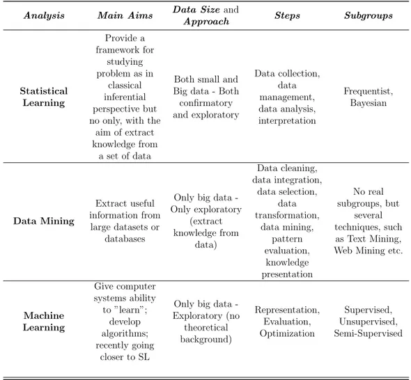
Table 1.1 Comparison between Statistical Learning, Data Mining and Ma-chine Learning

Analysis Main Aims Data Size and

Approach Steps Subgroups

Statistical Learning Provide a framework for studying problem as in classical inferential perspective but no only, with the

aim of extract knowledge from

a set of data

Both small and Big data - Both confirmatory and exploratory Data collection, data management, data analysis, interpretation Frequentist, Bayesian Data Mining Extract useful information from large datasets or databases

Only big data -Only exploratory (extract knowledge from data) Data cleaning, data integration, data selection, data transformation, data mining, pattern evaluation, knowledge presentation No real subgroups, but several techniques, such as Text Mining, Web Mining etc.

Machine Learning Give computer systems ability to ”learn”; develop algorithms; recently going closer to SL

Only big data -Exploratory (no theoretical background) Representation, Evaluation, Optimization Supervised, Unsupervised, Semi-Supervised

(19)

1.2 Statistical learning methodological

chal-lenges for Big Data

The development of the data-driven decision-making (DDDM) (Provost and

Fawcett, 2013) approach involves making decisions that are based on

ob-jective data analyses, in the sense that business governance decisions are undertaken only if backed up with verifiable data. This approach excludes so the influence of intuitive decisions or decisions based on observation alone. Big Data are the core of several DDDM analyses, increasing the size and the heterogeneity of available data to be used in such analyses. With such vast amounts of data now available, and estimating an exponential increase of that amount in the next years, companies in almost every sector are deepen-ing techniques and methodologies to exploit data information for competitive

advantage (Mallinger and Stefl, 2015). So, bbbb the paradigm shift in

sta-tistical learning has been encouraged not only by academics and researchers, but also by the expectation of businessmen and entrepreneurs, that have been involved in this fast and radical change, and are facing this increasing amount of data playing an active role. In literature, the wide use of big data analysis in order to obtain predictive power and so gaining advantages in terms of revenues, is often called as Big Data Predictive Analytics (BDPA) (Dubey

et al., 2017). To deal with the recent availability of big data, new

perspec-tives about data analysis have been inspired from several fields, leading to the development of new (or modified) statistical techniques. Therefore, new theoretical framework has been developed, as well as new ways to accomplish practical analyses. Thus, both innovations, theoretical and practical, have lead to a paradigm shift in data analytics. As pointed out by Sinan Aral in

Cukier, 2010.

”Revolutions in science have often been preceded by revolutions in measurement.”

Therefore, it is reasonable to assume that the creation of new ways to store, measure, analyse, interpret (in one word, conceive) data is the basis that

stays at the foundations of a new paradigm (Kitchin, 2014). Some authors

have claimed that this new paradigm is the establishment of “the end of the

theory” (Anderson, 2008). This debate is centered around the data-driven

approach as a result of big data era, with a reborn of an empiricism that does allow researchers to mine and retrieve information from data without making explicit theoretical hypotheses. This is an epistemological controversial, that points out how statistics as a whole has to face a new paradigm. According

(20)

to Kitchin, 2014, the strong emphasis on big-data-driven analyses has sev-eral properties, or features, that help to overcome sevsev-eral shortcomings of traditional deductive approach:

Given that n → ∞, in big data framework it is possible to represent a whole domain and, consistently, obtain results belonging to the entire population.

There is less space for a priori hypothesis, and statistical models are less useful in this context.

Analysis is without sampling design and/or questionnaire design po-tential biases. Data are able to have a meaningful and truthful trait by themselves.

To the extreme, data meaning transcends context or domain-specific knowledge, thus anyone familiar with statistics and visualization could

be able to interpret them in an exhaustive way. If the analysis is

carried out taking into account mainly information included in data and retrieved directly from them, it means that context knowledge takes second place.

Thus, given all these factors, some questions come out about the role and the validity of the techniques embedded in the original inductive statistics tool-box. A major case is the wide discussion over the validity of the p-value in big data scenario. Proper ad-hoc developments and possible solutions can be

found in Hofmann,2015. Null hypothesis significance testing (NHST) is the

classical way in which inductive statistics confirms or disconfirms underlying hypothesis. The controversy around it, and as a result around p-value issues,

has been broadly discussed already in Nickerson, 2000. In case of n → ∞,

in the new paradigm some authors suggest to move from classical NHST in-terpretation of confidence interval and significance in general into confidence intervals for effect sizes, which are considered presumably the measures of

maximum information density (Howell,2011). Classical statistical inference,

in such paradigm, seems so to have lost the predominant role with its tradi-tional tools. Generally speaking, the interest has moved towards techniques that are able to reduce the data complexity, rather than found significant relationships or differences. This is mainly due to the fact that in ase of big data analysis the following conditions are true: target population is not defined in advance as in the traditional way, sampling theory has lost its dominant role as in classical inference procedures, p-value and NHST have to be used carefully ( due to the fact that when n → ∞ and so even very

(21)

small discrepancies should be significant), data sources and data nature are

numerous and heterogeneous. As also pointed out in Franke et al., 2016,

it is almost obvious that in such scenario the focus of statistical analyses is on dimensionality reduction and in finding salient units to summarize main patterns. This work tries to give a contribution in such direction.

1.3 Big Data: a very brief history

As claimed by Zikopoulos, Eaton, et al.,2011:

“In short, the term Big Data applies to information that cant be processed or analyzed using traditional processes or tools. In-creasingly, organizations today are facing more and more Big Data challenges.”

Which kind of organizations are we talking about? Who was the first com-pany to make aware use of big data? Who was the first scholar to come out with a formal definition of big data? The answers to these questions are neither obvious nor easy. Probably, not even so useful. As said, the paradigm shift has been pretty fast and driven by a key development of available technology, which has affected everybody, academy and companies. A brief history of big data is useful to figure out the general path, and to understand what are the new challenges in terms of fields of application.

According to some authors, for example Barnes, 2013, the issues related to

modern big data framework and paradigm shift are, overall, a prosecution of past debates around several statistical themes. He has framed its specula-tions in his own geographic field research. By the way, given that big data are usually generated continuously, quickly and in large numbers, some fields can be considered as the most important natural sources of big data. In the following, 5 of the most relevant sources for big data are summarized:

Media technology. Data are complex (images, videos, sounds) and are generated very fast by electronic devices. A key role is played by social media platforms (Facebook, Twitter, Instagram and so on).

Cloud platforms. These platforms are designed for storing massive amount of data. Cloud platforms can be private, public or third party. Web in general. This is probably the most obvious, still the most important. Most of the data available in the net are free and retrievable. Internet of Things (IoT). Data generated from the IoT devices and their interconnections. IoT is a system of interrelated computing devices,

(22)

mechanical and digital machines, that are provided with the ability to transfer data over a network without requiring human-to-human or human-to-computer interaction.

Databases. In traditional form and in recent form. Structured or un-structured. For the most part, structured data are related to infor-mation with a very high degree of organization, whereas unstructured data is essentially the opposite.

In general, electronic devices like phones or IoT devices, produce massive, dynamic flows of heterogeneous, fine-grained, relational data. From a gen-eral perspective, it has been natural for companies acting in these fields to experiment an initial connection with big data analytics; academics involved in researches in that fields, as well, have conceived the new paradigm way earlier than others. Big data have, from that moment on, moved and influ-enced more fields year by year. Experts familiar with big data analytics have been able to apply the big data opportunities to new domains of application. For example, studies to improve benchmarking in medical sector have been

proposed in Jee and G.-H. Kim, 2013. The main purpose of the study is to

explore how and when use big data in order to effectively reduce healthcare concerns; especially for what concerns the selection of appropriate treatment paths, improvement of healthcare systems, and so on. For other public

sec-tors, a wide review can be found in (G.-H. Kim, Trimi, and Chung, 2014),

with a particular emphasis on enhancing government transparency and bal-ancing social communities. Governments and official institutions have avail-ability of a huge amount of data, especially collected in traditional forms, i.e. census data collection, but also an increasing capability to collect and analyze data that come from more recent sources, such as administrative sources. Data of different form (traditional, structured, unstructured, semi-structured, complex and so on), even if gathered from different sources, can belong to the same public sector, and their simultaneous analysis in order to obtain an exhaustive information retrieve process, is a hard challenge to face. The efficient use of big data analytics could provide sustainable solutions for the present state of art, and suggest future decisions to undertake, making a more aware use of information from policy makers. In the next section, challenges of the use of big data in educational sector will be deepen.

1.3.1 Big data in education and massive testing

In the contemporary era of big data, authors interested about the relation-ships between the paradigm shift regarding innovative data analytics and educational system, often refers to the the concept of big educational data.

(23)

In Macfadyen, Dawson, et al., 2014, Learning Analytics (LA) is defined as the possibility of implementing assessments and feedbacks in real-time evalu-ation systems. Learning analytics provides higher educevalu-ation helpful insights that could advice strategic decision-making regarding resources distribution to obtain educational best-performances. Further, the aim in this context is to process data at scale that are focused mainly on improvement of pupils’

learning and to the development of self regulated learning skills, under

the assumption that to improve cognitive skills it is necessary to customize learning process with respect to teachers and students needs and require-ments.However, also in this field, to accomplish these kinds of aims, a shift in culture is needed: from assessment - for - accountability to assessment

for learning (Hui, G. T. Brown, and S. W. M. Chan, 2017). In the former,

the evaluation is made because it is just a duty to accomplish, also because there is a law that makes it mandatory, and so people involved in a given system are aware that they have to carry out a process of evaluation. In the latter, efforts are made to use evaluation findings to undertake new policies, with the aim to improve future learning processes in school system. The new possibility to make use of big data analytics tools has become the major

innovation in order to reach that cultural change. In Manyika et al., 2011 it

has been outlined how data in general expands the capacity and ability of organizations, even public sectors, to make sense of complex environments, and educational system belongs without any doubt to the group of complex environments. Due to budget restrictions and increasing heterogeneity in learners, scholastic programmes and teachers’ background, several authors has claimed that using Learning Analytics in big data era is not a potential advantageous option but indeed an imperative that each organization has to

pursue (Macfadyen and Dawson, 2012). This kind of approach will lead to

optimize educational systems, making an efficient use of funds allocated for schools, highlighting good and bad practices mining information from data

(Mining, 2012). A key role in that sense is played by Learning Management

Systems (LMSs) (M. Brown,2011). Several researchers and technical reports

corroborates how learning management systems have the ability to increase student sense of community (both at scholastic and university level). Fur-ther, they can help to provide support in learning communities and enhance student engagement and success.

One of the most important and well-known source of big data in

educa-tion is worldwide the PISA assessment in OECD organizaeduca-tion framework 1.

Its main aim is to assess, by means of standardized and comparable tests, pupils’ learning/cognitive skills across the world. The core of PISA tasks can

1

(24)

be summarized with the words of OECD secretary-general Angel Gurra 2_:

”Quality education is the most valuable asset for present and future generations. Achieving it requires a strong commitment from everyone, including governments, teachers, parents and stu-dents themselves. The OECD is contributing to this goal through PISA, which monitors results in education within an agreed frame-work, allowing for valid international comparisons. By showing that some countries succeed in providing both high quality and equitable learning outcomes, PISA sets ambitious goals for oth-ers.”

These ambitious goals can be seen as benchmarking best-performances to look forward. As well as scholastic performances in terms of proficiency by itself, PISA tests data are also addressed to figure out how specific sociolog-ical, cultural, economical and demographic variables are able to affect the overall pupils’ results.

From all these hints and previous researches, it is clear that:

i Big data are available also in educational system, both from official institutions (such data from Minister of Education) as well as from tests to assess pupils’ skills.

ii New statistical learning paradigms go in parallel with new cultural framework in education: from assessment - for - accountability to as-sessment - for - learning.

iii It is becoming crucial to adopt decisions based on big data analytics, and expectations are that policy makers use findings from big data in conscious way. From policy makers perspective, it is not only advanta-geous to use such findings, but somehow mandatory nowadays.

iv Learning processes can be improved if results are correctly used and interpreted, leading to a customization in learning processes.

v Proficiency tests like PISA, the one carried out by OECD, but many others all around the world, are crucial sources of big data in education, and proper tools should be created and checked to analyze such tests. This work aims to address the last item since it presents a new tool to study complex data in education, showing it in action on real data and in particular to the Italian case of proficiency scores grouped by school.

2

(25)

1.4 Introduction to Symbolic Data Analysis

If data are made up by n objects or individuals, where each generic unit i is defined by a set of collected values from different variables of size k,

with a generic variable j, data matrix has the classic structure X(n,k) (1.1).

In contrast, symbolic data with measurements on k random variables are

k-dimensional hypercubes (or hyperrectangles) in Rk, or a Cartesian

prod-uct of k distributions, broadly defined (Billard and Diday, 2006). A single

point unit is therefore a special, and the simplest, case of symbolic data, that

leads to the described classic form of matrix (1.1) SDA provides a framework

for the representation and interpretation of data that comprehends inherent variability. Units under analysis in this approach, usually called entities, are therefore not single elements, but groups (or clusters, or set of units) gathered taking into account some given criteria. This leads to consider that there is an internal variation within each variable for each group. Furthermore, when dealing with concepts, such as animal species, pathologies description, ath-letes types, and so on, data involve an intrinsic variability that can not be neglected.

Each observation in SDA has, thus, a more complex structure, with this internal variation that has to be taken into account; while dealing with sim-ple points, only variation between observations is the core of the analysis. In SDA approach, the intrisic and comprehensive structure of observations leads to deal with within variation, as additional source of variability. From an interpretative point of view, symbolic objects plays a key role in statis-tics for complex data, cause they are suited to model concepts. This is a notion that has been developed inside Formal Concept Analysis (FCA), that is a framework laying mainly on the borders of Ontology and Information Systems, of which the first founder is considered Rudolf Wille in the early

80s (Wille, 1982). The original motivation of FCA was the aim to find for

real-world situations and contexts a confirm of mathematical order theory. FCA deals with structured data which describe relationship between units and a peculiar set of attributes/characteristics. FCA aims to produce two different kinds of output from the input data. One is a concept lattice, that is an agglomeration of concepts described in formal way contained in the data, usually hierarchically ordered using subconcept-superconcept relation

(Belohlavek, 2008). Such formal concepts are intended as representation of,

basically, natural concepts that human beings have in mind in an intuitively way, such as “mammal organism”, “electric car”, “number divisible by 2 and 5”, and so on. The second finding of FCA is the attribute implications, that describes the way in which a particular dependency, included in data, comes from formal concepts; e.g., “respondent with age under 15 are at high

(26)

schools”, “all mammals in data have 4 feet”, and so on. Many authors tried to figure out a valide hierarchical structure for the framework (i.e. Priss,

2006); to be more precise, in FCA formal concepts are defined to be a pair

(E, I), where E is a set of objects (called the extent ) and I is a set of at-tributes (the intent ). A category is a specific value assumed by a categorical variables, that so defines a group of units belonging to the same kind (such as birds of the same species). A class is a set of units, that are analyzed in the same context and once merged together form an unique dataset. Concepts are therefore the more complex structure in this theoretical thinking, and that’s where the significant role of Symbolic Objects come from.

From a pure philosophical and ontological point of view, authors claim (Bock

and Diday, 2000), that a great advantage of symbolic data analysis is that

symbolic objects thus defined are able to make a synthesis of the following different theoretical tendencies that are cornerstones in the ontological tra-dition:

Aristotelian Tradition

The link is in the fact that symbolic concepts can have the explana-tory power of logical descriptions of the concepts that they represent, given that concepts are characterised by logical conjunction of several properties.

Adansonian Tradition

Since the units of all the extension of a symbolic object are similar in the sense that they satisfy the same properties as much as possible, even if not necessarily Boolean ones. In that sense, the concepts that they represent are polythetic, so they cannot be defined by only a conjunction of properties, but members of same group will share most of the properties. This because in Adansonian Tradition a concept is characterised by a set of similar individual.

Rosch prototypes

Cause their membership function is able to provide prototypical in-stances characterized by the most representative attributes and individ-uals. So, prototypes will be the typical-type inside a given community, according to its features able to represent the category.

Wille property (FCA)

This property refers to the fact that an object is wholly described by

means of a Galois lattice (Ganter and Wille, 1996) Given that SDA is

derived directly from FCA, the so - called “complete symbolic objects” of SDA can be proved to be a Galois lattice, so this property is satisfied.

(27)

Symbolic data can be of different natures: intervals, histograms, distribu-tions, lists of values, taxonomies and so on. According to the given na-ture of the data, different techniques and approaches are developed in order to analyze them, and some examples of well - known symbolic data are in

(1.2), showing different kind of visual representation. A formal definition

of symbolic variable in presented in Bock and Diday, 2000. A

comprehen-sive ontology of the different nature of symbolic variables is proposed by

Noirhomme-Fraiture and Brito, 2011, where variables are first of all divided

between numerical and categorical, and then hierarchically partitioned due

to their nature, as depicted in 1.1.

Figure 1.1: Ontology of symbolic variables, taken from Noirhomme-Fraiture

and Brito, 2011.

In case of interval data, i.e. _{data expressed by interval of R, a pair}

of numbers [a, b] represents all the numbers a ≤ x ≤ b. One of the first proposed formalization to deal with such data was the interval arithmetic

(Moore, Kearfott, and Cloud, 1979), that has introduced and defined

al-gebraic properties and has proposed metric for such data. In particular, authors have started to conceive the fuzzy set theory (Moore and Lodwick,

2003) linked to the analysis of interval data. In case of categorical data,

a remarkable approach is the one related to compositional data (Aitchison,

1982). A compositional data point is a representation of a part of a whole,

like percentages, probabilities or proportions. Usually it is represented by a positive real vector with as many parts as considered. For example, if we look at the elements that compose the Planet Earth structure, we see that in first place there is iron (32.1% ), followed by oxygen (30.1% ), silicon (15.1% ), magnesium (13.9% ), while all the others elements account for 8.8% . There-fore, a compositional way to represent the data point ”Earth” is vector of 5 elements: [0.321, 0.301, 0.151, 0.139, 0.08]. A dataset of compositional data,

(28)

(a) ZoomStar for different kind of Symbolic data (9 interval data, 3 multinomial or distributional data) in cars dataset. Credits to the R package symbolicDA

(b) Histogram-value data of some countries by age and gender, represented by means of Histogram. Credits to the R package HistDAWass

(29)

in this example, will be made up by a different in each row , resulting then in a vector of length 5 as observed value .

In the following section, the algebra and the features of distributional/his-togram valued data will be deepen.

(30)

(31)

Chapter 2 Elements of Distributional and

Histogram-valued Data

2.1 Distributional Data and Histogram-valued

data in SDA

Distributional Data are a specific kind of data embedded in SDA. Each ob-servation is defined by a distribution, in the wide sense of the term. It can be a frequency distribution, a density, a histogram-valued data or a quantile function. Such data are assumed to be a realization of a numeric modal symbolic variable. In particular, modal variables can model the description of an individual, of a group, or of a concept, by probability distributions,

frequencies or, in general, by random variables (Irpino and Verde, 2015).

For example, data retrieved from official statistics as macrodata, are usually described by means of basic statistics. When estimating a parameter, the estimation is presented under the distribution of such estimation in several samples. In these cases, even if we are observing a single variable, the proper expression of such variable is not a single value but instead a multi-valued quantity.

According to the literature (Bock and Diday,2000, Noirhomme-Fraiture and

Brito,2011), for histogram symbolic data we consider the situation in which

the support is continuous and finite, and each observed value is an histogram

developed over such continuous finite support, as in 1.2. To deepen the

structure of numerical nature of symbolic variables, each quantitative vari-able, from a general perspective, may then be single-valued (real or integer) as in the in classical framework, if it exspresses one single value per observa-tion. Moving to the proper domain of SDA, a variable is multi-valued if its values are a finite vector of numbers belonging to a finite numerical support.

(32)

Further, interval variable occurs if its values are intervals (Moore, Kearfott,

and Cloud, 1979). Usually, when dealing with an empirical distribution over

a set of subintervals, the variable is called a histogram-valued variable. Let’s define X as the variable, D as its underlying domain and R as its range, i.e. where is theoretically possible to express its values. Given a set of statis-tical units of size n, S = (s1, s2, ..., sn), in SDA framework, is possible to sum

up the information contained in S by means of an application, leading to the symbolic variable X made up by p different variables, and with i = 1, ..., n:

X : S → D such that si → X(si) = α (2.1)

where α is the single numeric result of the application and D ⊆ R. It means that, with such application to S, all the values of the range R are still plausible, and are equal to the entire domain D. This is, given that only one α is the outcome, the simplest case of SDA, when it becomes a single standard numeric variable with only one realization for each observation.

When, on the other hand, values of X(si) are finite sets of αi, (2.1) becomes:

X : S → R such that si → X(si) = (α(1i), α(2i), ..., α(pi)) (2.2)

leading to a finite set of realization for each observation i. The defined

vari-able deriving from (2.2) is a multi-valued ones, so. The application creates

a finite set of values that describe the statistical unit. In case of interval-valued data, the application leads to:

X : S → R such that si → X(si) = [li, ui] (2.3)

I is in this case a (n × p) matrix containing the values of p interval variables on S. Therefore, each p-tuple of intervals Ii = (I(i,1), I(i,2), ..., I(i,p)) defines

a specific si ∈ S. Lastly, histogram-valued data are in this approach made

up by aggregating microdata in several intervals (or bins) inside lower bound

and upper bound [li, ui], providing more information than interval data about

data distribution.

X : S → R such that si → X(si) = [Ii1(p1), Ii2(p2), ..., Iik(pk)] (2.4)

In this context, [Ii1, Ii2, ..., Iik] are the set of sub-intervals, associated with the

observed frequencies (p1, p2, ..., pk). Therefore, it could be deepen the

analy-sis of internal variation between the maximum and the minimum value of the

distribution, while in interval data in (2.3) is not possible to make specific

assumption about frequency distribution, but only about general distribution between boundaries. Further, the usually hypothesis made for in histogram-valued data, is that in each subinterval data are uniformly distributed. Of

(33)

course, if there is only one bin in the histogram structure, (2.4) simplifies

in (2.3), and therefore interval-valued data are a special case of

histogram-valued data.

2.1.1 Main statistics for histogram-valued data

The issue of histogram-valued data, and symbolic data in general, when try-ing to calculate basic descriptive statistics, is the nature itself of such data

(Irpino and Verde, 2015). Each descriptive statistic has to take into account

the degree of internal variation that exists inside observations, while in single-valued data only between observations variation is considered. So, questions arise about to the extent to which classical formalization and classical con-cepts of descriptive statistics can be adopted in case of distributional data. The central core of the different approach is, then, the dispersion evaluation

inside each observation. As introduced in 2.1 and formalized in (2.4), inside

each bin (sub-interval) of the histogram data are considered to be distributed as an uniform random variable. So data are equally spread from lower bound of the bin to the upper bound of such bin. Formally, for each h interval where h : (I1, I2, ..., Ih, ..., Ik): φiX = X j<h pji+ phi· x − lji uji− lji where (j = 1, ..., k) (2.5)

where φi is the density distribution for the variable X calculated in i. We,

thereafter, consider the definition proposed in (ibid.) for distributional

sym-bolic variable:

Definition 2.1.1. A modal variable is called a distributional symbolic

vari-able if for all i the measure φi has a given density φi, and so is possible to

simplify the relationship as: Xi = φi.

The debate about univariate and bivariate statistics for histogram-valued data is a consequence of the starting approach and the theorized paradigm that is behind the formalization of such distributional data. In SDA a com-mon groundwork is that there are two different level of real data collection

(Bock and Diday, 2000). First level, the lowest one, is related to elementary

units. Aggregating together micro-data from basic units leads to obtain up-per level data. This kind of histogram-data are so considered a generalization of observed values in a group of lower-level units. The analysis procedure that moves the computation from first level to second level has been deepen

(34)

assumptions are expressed about a generic set N formed by a number n of elementary units. It can be fully described by a distribution-valued variable

X, with Xi = φi. Going straightforward to the statistics, it implies that the

mean, the variance and the standard deviation are the result of such statis-tics computed on a mixture of n density functions, one for each observation in the set N containing 1-level units. Usually, if all units are equally likely

to be present in N , weights used to create the mixture are all equal to _n1.

As presented in (Fr¨uhwirth-Schnatter, 2006), resulting mean of the mixture

Pn i=1 1 nφi = φ is: E(X) = µ = n X i=1 1 nµi (2.6)

Further, variance is defined as:

E[(X − µ)2] = σ2 = n X i=1 1 n(µ 2 i + σ 2 i) − µ 2 _(2.7)

In this approach, symbolic distributional data are suited to represent real situation in which group of individuals are the basis to form an upper level entity (employees nested in companies, pupils nested in schools and so on). It is, of course, a context that happen pretty often, therefore the 2-level paradigm has a wide range of possible application in real life, cause data that are naturally organized in hierarchical order are not uncommon. Fur-ther, if previous knowledge are available, is possible to change the weights to calculate the φ mixture giving more importance to groups that are known, for example, to be larger. Anyway, univariate statistics thus conceived are implicitly assuming that there is no significant difference between individuals inside the same group, or, at least, this kind of paradigm is not able to catch such heterogeneity. Indeed, switching values assigned to different individuals belonging to the same group, overall means and variance don’t change. This framework does not allow to compare individuals aside from their groups. In descriptive statistics context, mean (as expected value) can assume sev-eral definition and formalization to extend straightforward its properties and formalization to different kind of data. If we take into account recent develop-ments and formalization of Frechet mean (Ginestet, Simmons, and Kolaczyk,

2012; Nielsen and Bhatia, 2013) such that:

Definition 2.1.2. with n elements described by the variable X, a di distance

between two descriptions and a set of n real numbers Z = (z1, ..., zn), a

Frechet type mean (known as barycenter ) MF ris the argmin of the following

function: MF r= arg min x n X i=1 zidi2(xi, X) (2.8)

(35)

The minimization problem in 2.8, is a generalization problem of finding an entity of central tendency in a cluster of points (also called centroid ). Other kind of means, such as harmonic or geometric means, are just the

ex-tension of the 2.1.2 using different kind of distance di.

Chisini mean (Graziani and Veronese, 2009) applies another approach to

the definition of a mean. Often authors refers to the Chisini mean as

rep-resentative or substitutive mean (Dodd, 1940), due to its definition that is

considered to be useful in practical context. Formally:

Definition 2.1.3. a Chisini mean of single-valued variable X and a function F such that F (x1, ..., xi, ...xn) applied to a set of n object, the mean is defined

as:

F (x1, ..., xi, ...xn) = F (Mchisini, ..., Mchisini, ..., Mchisini) (2.9)

where (Mchisini, ..., Mchisini, ..., Mchisini) is a vector that is the mere repetition

of the Chisini mean n times.

Due to some analytical issues, the equation in (2.9), could not have a

finite solution, and further the Chisini mean could be external to the interval

of observations [xmin, ..., xmax]. Consequently, usually some constraints are

imposed to the function F in order to obtain an unique final solution to the minimization problem.

It has to be pointed out that, to extend both Chisini and Frechet means to distributional variables, first step is to define a proper distance measure between distribution (as histogram-valued data). Several dissimilarity and distance measures between such symbolic data have been proposed (J. Kim,

2009) and compared to each other by several authors. The underlying idea

about the overall comparison of two histogram-valued data in SDA is that the comparison has to take into account way more statistical aspects than in the comparison between two single-valued data. For example, given the different internal variation inside each distributional observation, two his-tograms could share even same mean and/or median, but nevertheless have a dissimilarity (or a distance) > 0. This can be due to a different degree of dispersion, in terms of variation, around a fixed central tendency index. Therefore, the basic idea behind distributional distances is that they should be able to compare much part of distributions as possible.

Some of such dissimilarity measures come from the extension of a given dis-similarity measure suited for interval-valued data, and then developed to deal with histogram-valued data. The underline assumption is that is

pos-sible moving from (2.3) and extend that formalization to (2.4), and so that

if a measure is valid to compare two intervals, it is as well a proper choice to compare two groups of intervals (each of them being an histogram). To

(36)

formalize such kind of measures embedded in this approach, in the following we define intersection and union between histogram objects taking into ac-count their relative frequencies p linked to the nb number of bins. For this formalization, histograms are assumed to be adequately transformed in order to have exactly same sub-intervals.

Definition 2.1.4. For two different histogram object Hist1and Hist2, where

for each bin there are relative frequencies such that Hist1 → (p(1,1), p(1,2), ..., p(1,nb))

and Hist2 → (p(2,1), p(2,2), ..., p(2,nb)), intersection between them is defined as:

Hist1∩ Hist2 = p1,i∩ p2,i, with i = 1, ..., nb (2.10)

where each p1,i∩ p2,i = min

1,...,i,...,nb(p1,i, p2,i) (2.11)

Therefore, from (2.11) we formalize the concept of intersection as a

com-parison, bin by bin, of their respective density, and considering only the amount of shared density. From a graphical point of view, such shared

den-sity is the only part in which histograms bins overlap2.1.

Further, union between histogram objects is defined consequently as:

Definition 2.1.5. For two different histogram object Hist1and Hist2, where

for each bin there are relative frequencies such that Hist1 → (p(1,1), p(1,2), ..., p(1,nb))

and Hist2 → (p(2,1), p(2,2), ..., p(2,nb)), union between them is defined as:

Hist1∪ Hist2 = p1,i∪ p2,i, with i = 1, ..., nb (2.12)

where each p1,i∪ p2,i = max

1,...,i,...,nb(p1,i, p2,i) (2.13)

So, union thus defined leads to compare as well bins densities one by one of both histogram, but the result is the maximum value that such density shows. It is worthy to note that the sum of across bins densities in case of union is ≥ 1, while on the other hand sum of such densities in case of intersection is ≤ 1.

2.1.2 Main dissimilarity/distance measures for

histogram-valued data

Some dissimilarity measures take into account, in their calculation, elements from both intersection and union between histograms, and that’s why is use-ful to introduce them as part of histogram algebra. Further, some extensions of dissimilarity measures that developed from interval to continuous data, include concept of mean and standard deviation derived from formalization

(37)

Figure 2.1: Two histograms and their overlapping densities. Intersection as

defined in (2.1.4) is the purple part where they overlap, union as defined in

(38)

of Billard and Diday (2003). It starts from the general assumption of uni-form distribution in each sub-interval. So, to compute the mean inside each

of them it has to be applied a simple arithmetic mean between boundaries li

and ui. Formally:

Definition 2.1.6. Given an histogram object Hist that is made up by nb

number of bins and as in2.3 with li the lower bound of such bins and ui the

upper bound, mean according to Billard is defined as:

MHist = nb X i=1 li+ li+1 2 pi (2.14)

Therefore, as mentioned, mean in (2.14) is a weighted mean (using

ob-served density) of central values across bins. Standard deviation start from

same assumption, and as formalized in (J. Kim,2009):

Definition 2.1.7. SDH. = v u u t nb X i=1 (li− MH.)2+ (li− MH.)(ui− MH.) + (ui− MH.)2 3 pi (2.15)

These formalization are valid in case of natural histogram-valued data. When dealing with objects coming instead from a previous procedure of union or intersection of histogram objects, such definitions need a correction due

to the fact that, as mentioned, (2.6) has to hold thatPnb

i=1pi = 1. In case of

union as defined in (2.1.5) such sum isPnb

i=1pi > 1 and in case of intersection

from (2.1.4), Pnb

i=1pi < 1. Therefore, we introduce the quantity p∗ that is

the normalization of such sum in order to obtainPnb

i=1pi = 1.

p∗_(Hist

1∪Hist2)i =

p(Hist1∪Hist2)i

Pnb

i=1p(Hist1∪Hist2)i

(2.16)

p∗_(Hist₁_∩Hist₂_)i = p(Hist1∩Hist2)i

Pnb

i=1p(Hist1∩Hist2)i

(2.17) Therefore, mean and standard deviation of objects derived from union or

intersection of histograms will take into account definitions in2.16and2.17to

have estimation of such univariate statistics consistent with usual properties. Definition 2.1.8. Mean for an histogram-valued object derived from union or intersection of simple histogram-valued objects are computed as:

M_{(Hist1∪Hist}∗ ₂₎ = nb X i=1 li+ li+1 2 p ∗ (Hist1∪Hist2)i (2.18)