Technical Report CoSBi 19/2007
Simplifying the Stochastic Petri Nets
Formalism for Representing Biological
Phenomena
Ivan Mura
The Microsoft Research - University of Trento Centre for Computational and Systems Biology
Simplifying the Stochastic Petri Net Formalism
for Representing Biological Phenomena
Ivan Mura
The Microsoft Research - University of Trento Centre for Computational and Systems Biology
mura@cosbi.eu
Abstract
This paper proposes a simplification of the stochastic Petri nets graphical notation with the purpose of defining a more compact and clearer graphical way of building formal models of biological phenom-ena. Three biological examples are first presented, then modeled with the classical SPN modeling formalism, and their key modeling patterns distilled to identify the main features that need to be represented in a stochastic model. The key features are then the object of the original part of the paper, in which a simplified and more concise, although formal, graphical notation, is proposed, and applied to the selected examples. The paper demonstrates the effectiveness of the simplified notation in producing more compact and understandable models of biological phenomena, still retaining the nice properties of Stochastic Petri Nets, i.e., their flexible abstraction level and formal semantics.
1
Introduction
Many different languages and tools are being used in Systems Biology to formalize in a structured way characteristics of biological phenomena and to produce models amenable to qualitative and quantitative analysis. Just to mention some of them, systems of coupled ordinary differential equations, statistical tools, statecharts, process algebra based languages and stochastic state-based formalisms such as Petri nets, are all subject of active research and application. Each of them meets some needs of this scientific field, with relative merits and weaknesses.
Several of the tools mentioned above only have a short history of appli-cation to the biological domain. Indeed, statecharts [11], process algebras [3] and Petri nets [18] were initially proposed as tools for representing con-current systems in computer science domains, and their applicability to the modeling and analysis of biological phenomena has only started in recent years.
We shall focus in this paper on stochastic Petri net (SPN, hereafter) modeling formalisms, for which the first example of application to biology dates to less than 10 years ago [10]. SPN models have since then been ap-plied to various biological research problems, and several papers have been published showing their applicability, see for instance [19, 20, 16, 17]. More-over, other types of Petri nets based formalisms, such as Hybrid Petri Nets, are also being used for the analysis of biological systems, see for instance [15, 21].
A whole family of SPN formalisms has been developed in the computer science community. Generalized Stochastic Petri Nets [14], Colored Petri nets [13], Stochastic Activity Networks [7], Stochastic Reward Nets [6], Stochastic Well-Formed Nets [5], just to mention some of them, have been proposed, and various tools developed to provide graphical user interfaces and analytical and simulation support to model definition and solution. Many of these proposals originated from attempts to limit the sometime cumbersome graphical notation of basic Petri nets, with the addition of more expressive modeling constructs. Quite interestingly, there has been a scant transfer of such higher level SPNs into the research communities of biologists, apart some exceptions, see for instance [10]. In particular, the possibilities offered by the explicit representation of the so-called marking-dependence have not been consistently exploited yet for the modeling of biological systems. Because of this, models tend to be larger, less readable and less structured than they could be.
eas-ily stretch state-based modeling tools to the limits of their capabilities, and the term state-space explosion is a very appropriate way to describe the combinatorial growth of the size of the stochastic process underlying the user-defined models. Such stochastic process, usually an continuous-time Markov chain, is the actual object of the model evaluation step (conducted either analytically or via simulation). However, for a tool using a graphical representation formalism, such as Petri nets, dealing with big size mod-els also poses challenges because user-defined modmod-els may quickly become unmanageable and unreadable by people other than the author. We will present in this paper some examples of toy systems and will demonstrate the level of intricacy that their SPN models can exhibit. This issue has led to various attempts to add expressiveness to Petri net tools, so to provide compact representation of complex behaviors, notably exploiting symmetries and regularities (see for instance Colored Petri Nets and Well-Formed Nets) and introducing marking dependent constructs that allow capturing into higher level mathematical constructs quantitative behaviors and constraints otherwise represented with additional graphical elements.
The primary objectives of this paper is to simplify, still with keeping un-changed the formal semantics of the models, the graphical notation of SPNs, so that it will be easier to build formal models that suit the needs of biolo-gists. To this goal, this paper proposes to get rid of all of the unnecessary graphical elements that get usually included in Petri net models of biolog-ical systems and that are actually not carrying any particular information associated to them. In this simplification process, we will be considering the standard representation practices of biologists, who have developed a semi-standardized graphical notation to model the available information about the known interactions that exist between biochemical species. Also, to fur-ther streamline models, we will convey into the simplified graphical notation some of the most expressive features of high-level SPN formalisms.
We will approach the simplification process in the paper by first describ-ing threecase studies of biological phenomena and modeling them with the basic SPN modeling constructs. We will then use those three examples to support the identification of the aspects of the notation that can be object of the simplification. Finally, we will apply the simplified notation to the three case studies to visually compare and comment on the different form of the original and of the simplified models.
The rest of this paper is organized as follows. We first introduce in Section 2 the three biological case studies we will be using throughout the paper. Then, we briefly recall the key elements of the SPN modeling formal-ism in Section 3 and apply the formalformal-ism to model the three case studies in
Section 4. Drawing from the typical features of biological systems that get modeled in the three examples, we present in Section 5 the simplified no-tation, whose application is demonstrated in Section 6. Finally, we provide some concluding remarks, comparison with other recent attempts to define a notation for systems biology and directions for future work in Section 7.
2
Biological examples
2.1 The MAPK signaling cascade
We describe in this section a simple instance of the mytogen-activated pro-tein kinase (MAPK), a signaling cascade whose intermediate results cause the sequential stimulation of several protein kinases [12]. The stages of this signaling cascade contribute to the amplification and specificity of the transmitted signals that eventually activate various regulatory molecules in the cytoplasm and in the nucleus. Initiation of cellular processes such as differentiation and proliferation, as well as non-nuclear oncogenesis are all affected by the MAPK signaling cascade.
The following is a simplified view of the intra-cellular MAPK cascade. The signal transmission involves three protein kinases, called MAPKKK, MAPKK and MAPK. MAPKKK is a MAPK kinase kinase, which, when active, is able to perform two steps of addition of one phosphate group (-PO3) to the MAPK kinase MAPKK. Doubly phosphorylated molecules
of MAPKK are in turn able to perform two steps of addition of a phos-phate group to molecules of MAPK. The doubly phosphorylated molecules of MAPK represent the final product of this signaling cascade.
Signals that initiate the cascade are not precisely known yet. It is assumed that MAPKKK is activated and inactivated by two enzymes E1 and E2, respectively. Moreover, each phosphorylation step of MAPKK and MAPK is reversible, in that specific phosphatases are in fact competing with the phosphorylation process, removing phosphate groups from MAPKK and MAPK.
2.2 E. coli heat-shock circuit
A variety of different stresses, including both heat and chemical shock, lead E. coli to activate a response that is initiated through the expression of genes coding for theσ32 protein [19]. Proteinσ32is an unstable sigma factor with a short half-life on the order of one minute, and it is able to complex with polymerase to form theσ32holoenzyme. Under normal circumstances,σ32is
out competed by sigma factorσ70, which results in low levels ofσ32mediated
response. However, under heat shock conditions, the concentration of σ32 increases and theσ32holoenzyme starts to actively transcribe various genes
coding for heat shock response proteins.
The heat shock response proteins, primarily DnaK, DnaJ and GrpE act as chaperones for misfolded/aberrant proteins. Moreover, it has been shown [8] that these three proteins are able to complex and the resulting complex can bind σ32 molecules. When bound to this complex, σ32 is presented to anotherσ32regulated protein, named FtsH, for degradation. This
degrada-tion pathway provides a means to maintain the concentradegrada-tion of σ32 to its
physiologically appropriate level.
2.3 Chemotaxis in E. coli
Chemotaxis is the ability of bacteria to move toward attractants (e.g. food or light) or away from repellents (e.g. poisonous substances). For the sake of simplicity, in the following we shall stick to the case when chemotaxis is directed to food sources. The chemotactical behavior has been subject to extensive studies in many organisms, notably in Escherichia coli, and has been found to be the result of evolution of a comparatively simple pathway [4]. The concentration level of the active (phosphorylated) form of a single protein, called CheY, is able to control the rotation sense of the flagellar motors in E. coli. The higher the concentration of phosphorylated CheY, the more frequently the bacteria tumbles (clockwise rotation of the motors). The lower the concentration of phosphorylated CheY, the more frequently the bacteria steadily swims in a precise direction (counter clockwise rotation of the flagellar motors). Dephosphorylation (inactivation) of CheY is mediated by a protein called CheZ.
The phosphorylation of the effector CheY in the bacteria cytoplasm is controlled by the presence of the active (phosphorylated) form of a histi-dine kinase CheA, which gets activated in the inner part of specific cross-membrane receptors. The external part of the receptors is able to bound the attractant molecules. The bound or unbound state of the external part of receptors changes the probability of activation of the internal part of the receptor. Such activation results in the auto phosphorylation of CheA molecules in the cytoplasm due of allosteric effects. Specifically, binding of a ligand molecule to the receptor reduces the probability of self activation of CheA. Active CheA molecules are able to transfer a phosphate group to an inactive (not phosphorylated) molecule of protein CheY. Because the phos-phorylated molecules of CheY increase the clockwise rotation of flagellar
motors and thus bacteria tumbling frequency, in an area poor of attractant the bacteria tend to tumble, whereas when a gradient of attractant is en-countered E. coli increases its swimming frequency to actively search for the source of food.
Moreover, E. coli chemotactical pathway also endows the bacteria with the ability of adapt to the conditions of the environment, meaning that the bacteria will tend over time to become insensitive to a stable concentration of the ligand. This behavior is mediated by another part of the chemotacti-cal pathway, which acts on the probability of self phosphorylation of CheA. Specifically, a phosphorylated molecule of CheA is able to transfer a phos-phate group to an inactive molecule of protein CheB. The active molecules of CheB are able to remove one methyl group (-CH3) from the receptors, which have four methylation sites. Each removal of one methyl group in-duces small structural changes in the receptor, which result in a reduced propensity for CheA self activation. However, active CheB molecules are able to cause this methylation only on active receptors. Therefore, under a condition of scarce ligand concentration, the tumbling frequency tends to decrease because the self phosphorylation of CheA is progressively in-hibited on unbound receptors and the bacteria starts swimming. Another process operates on receptors, mediated by protein CheR. CheR is able to add phosphate groups to inactive receptors. Therefore, in a condition of ligand abundance the swimming of bacteria is progressively reduced and the bacteria tend to tumble more and thus stop in the rich area.
Spontaneous de-phopshorylation (inactivation) of active molecules of protein CheB also occurs in the cytoplasm.
3
Petri net modeling formalism
Many variants of modeling notations exist for SPNs (a comprehensive list can be found at the web site [1] maintained by the University of Hamburg), therefore we shall first describe in this section the precise notation we will be using, to make sure that no ambiguities exist in the interpretation of the models. Before entering into the details of the modeled examples we shall also briefly recall the classical interpretation of Petri net modeling elements in biology.
We shall use the basic elements of Petri nets, i.e. places, transitions, arcs and tokens with following the standard graphical notation reported in Figure 3. The rules to compose correct SPN models from the basic modeling elements are the following ones:
Figure 1: Basic Petri net modeling elements
• tokens are only contained into places;
• arcs can only connect a place to a transitions or a transition to a place, i.e., the graph that represents the structure of the net is a bipartite one.
The number of tokens inside a place defines themarking of the place. The marking of the Petri net model is the vector that collects all the markings of the places in the model. A transition is said to be enabled if each of its input places, i.e. the places from which an arc exists going from the place to the transition, contain at least one token. An enabled transition fires in a random time. We shall stick to a specific distribution of the random variable representing the firing time: the negative exponential, completely described by a single parameterλ, called the rate.
The firing of a transition atomically removes one token from each input place of the transition and deposits one token in each of theoutput places of the transition, i.e. those places for which an arc exists going from the transi-tion to the place. Conflicts among enabled transitransi-tions, i.e. those situatransi-tions in which multiple transitions are enabled and these transitions share some input places, are resolved by using a race policy, i.e. the shortest random time among those of all enabled transitions is the one that determines which transition will fire. After the firing, the marking of the net is changed, a new set of transitions may be enabled for firing and if conflict still exist, a new race will occur. If an enabled transition gets disabled from a conflicting one, the memory of the elapsed time it has been enabled is lost, and at the next enabling a new random firing time will be sampled from the negative expo-nential distribution of the transition. However, notice that this rule, albeit useful for understanding the rules of concurrent firing, is unessential because of the memoryless property of the negative exponential distributions.
We shall also consider here theinhibitory arc, which can only link a place to a transition, and allows testing the marking of another place. All input places connected to the transition through inhibitory arcs must be empty for the transition to be enabled. The graphical representation of an inhibitory
arc is shown in the next picture.
Figure 2: Inhibitory arc notation
Moreover, we shall also allow arcs (normal and inhibitory ones) having assigned positive integerweights, (default 1, not indicated) which enrich the possibility of controlling the enabling of transitions and the token flow after transition firing. Specifically, a transition will be enabled if all the input places connected through normal arcs contain at least as many tokens as the weight of the connecting arc, and all places connected through inhibitory arcs contain less tokens that the weight of the connecting arc. When a transition fires, it removes from each input place as many tokens as the weight of the connecting arc, and puts as many tokens as the weight of the connecting arc inside each output place.
It is worthwhile observing the relative simplicity of the modeling for-malism, which deploys very few elements and at the same time is able to represent many complex behaviors. On the other hand, its simplicity makes the size of models to grow quickly as the system to be modeled gets complex and the readability (and consequently maintainability and verifiability) of models is impaired by a forest of arcs.
3.1 Petri net models for biological phenomena
Being an abstract modeling formalism, Petri nets per se do not refer to any specific aspect of the biological domain, but rather a meaning has to be associated by to modeler to places, tokens and transitions. In the context of biological phenomena, the classical interpretation of Petri net elements is the following one:
• Places represent chemical species or more complex biological entities as well, such as as ribosomes, receptors, genes.
• Tokens inside a place (the marking of the place) model the number of molecules of the species or of the entity represented by the place. Notice that tokens are anonymous entities that do not carry any qual-ifying information, and thus the molecule or the biological entity they
represent changes as they move from a place to another1. Notice that tokens are not always graphically depicted, apart from the cases in which there are a few of them, but rather they are associated to places when providing the initial state of the models.
• Transitions represent biochemical reactions. The exponential rate as-sociated to a transition expresses the speed at which a reaction occurs. By default, the firing follows the infinite server semantics, meaning that, if the number of tokens in the input places allows for multiple reactions to proceed concurrently, the rate of the reaction is multiplied by the number of the reactions, which is indeed quite a simple way of modeling chemical reactions obeying the mass-action law.
4
SPN modeling of biological examples
In this section, we shall use Stochastic Petri Nets formalism described above to define models of the selected examples of biological phenomena.
4.1 MAPK cascade model
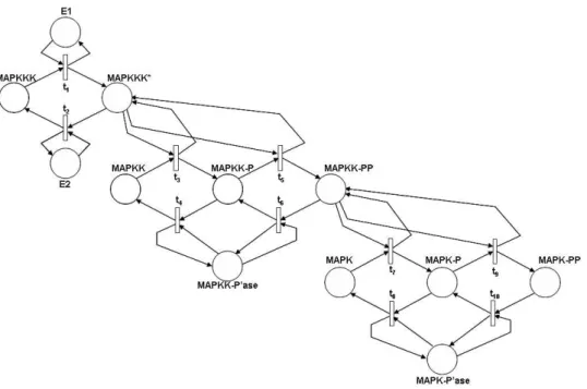
An SPN model of the MAPK cascade needs to account for the different biochemical species and their various phosphorylation states. Thus, the model proposed in Figure 3 has one place for E1, E2, MAPKKK and for its active state MAPKKK∗, MAPKK and its two phosphorylation stages MAPKK-P and MAPKK-PP, MAPK and its two phosphorylation stages MAPK-P and MAPK-PP. Moreover, the two placesM AP KK− P′ase and
M AP K − P′ase are also introduced to model the MAPKK and MAPK
phosphatases.
In the model, tokens contained in a place named X (the marking of X) represent the molecules of biochemical species X. Transitionst1andt2model
the activation and deactivation of MAPKKK, respectively. Each firing of transitiont1moves one token from placeM AP KKK to place M AP KKK∗. Moreover, because this biochemical transformation is actually driven by the presence of the signal E1, the place E1 is an input place for t1 as well. However, because E1 is not affected by the activation of MAPKKK, place E1 is also an output place for t1, which means that the marking of place
E1 will be not changed by the firing of the transitions. In quite a similar
1Some Petri net modeling formalisms (for instance Colored Petri Nets [13]) allow for
way, firings of transition t2 move tokens from place M AP KKK∗ to place
M AP KKK with sensing the state of place E2.
Figure 3: SPN model of MAPK cascade
The active molecules of MAPKKK mediate the addition of phosphate groups to MAPKK molecules. The two transitions t3 and t5 model the
addition of one phosphate group to molecules of MAPKK with moving one token from place M AP KK to M AP KK− P , and of one phosphate group to the already phosphorylated MAPKK with moving one token from place M AP KK− P to place M AP KK − P P , respectively. Because the addition of each phosphate group is mediated by the active form of MAPKKK, both the two transitions sense the status of placeM AP KKK∗.
The process of MAPKK dephosphorylation competes with the activity of transitions t3 and t5. Transitions t4 and t6 move tokes in the opposite direction, from places M AP KK− P to place M AP KK and from place M AP KK−P P to place M AP KK −P , respectively. Because the process is mediated by the MAPKK phosphatase, the two transitions sense the status of placeM AP KK− P′ase.
The final stage of the cascade, which changes the state of MAPK, is analogous to the previous one. The two transitions t7 and t9 model the addition of the first and of the second phosphate group to MAPK, and the
two transitionst8 and t10 model the removal of the phosphate groups. The
addition is mediated by the doubly phopshorylated form of MAPKK and the removal by the MAPK phosphatase, which is modeled in the SPN by the arcs from/to placesM AP KK− P P and M AP K − P′ase.
4.2 σ32 pathway model
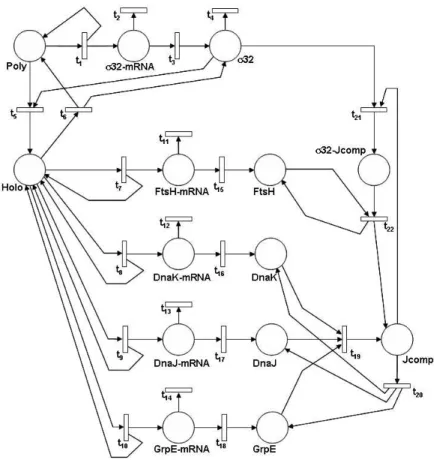
An SPN model of theσ32pathway described in Section 2.2 is shown in Figure
4. This model is largely taken, with slight modifications, from the one by Srivastava et al. presented in [19]. In this example, the places of the model account for the proteins composing in the pathway, plus their mRNAs and finally the polymerase and the σ32 holoenzyme. For the sake of simplicity,
we shall not consider the processes of nucleus/cytoplasm translocations and will make the assumption that each mRNA molecule is either degraded or translated into the encoded protein, but the translation may occur only once and after that the mRNA molecule is degraded anyway.
Tokens in placeP oly represent molecules of DNA polymerase. A molecule of polymerase activates the transcription of the gene (not represented in the model) coding for theσ32factor, and transition t1 models the transcription event. Obviously, polymerase is not consumed in the process and therefore place P oly is also an output place of transition t1.
Tokens in placeσ32− mRN A represent molecules of the mRNA for σ32. Transition t2 represents the degradation of a σ32 mRNA molecule, and the competing transition t3 models the translation of the σ32 mRNA molecule
into the protein. Tokens in placeσ32 model the molecules of σ32 in the cell and transitiont4 represents the degradation ofσ32.
Transition t5 andt6 model the complexation and decomplexation ofσ32
and polymerase molecules, respectively. The output of a complexation event is one molecule of theσ32holoenzyme, which is represented in the model by a token in placeHolo.
The holoenzyme activates the transcription of genes coding for Ftsh, DnaK, DnaJ and GrpE proteins, which is captured in the model through transitions t7, t8, . . . , t10. Each of these transition outputs one token
rep-resenting one molecule of mRNA, which is deposited in the relevant place. Again, the molecules of the holoenzyme are not consumed in this process, and thus the place Holo is an output place for transitions t7, t8, . . . , t10.
Transitionst11, t12, . . . , t14 model the degradation of the mRNA molecules, whereas transitions t15, t16, . . . , t18 represent the translation of the mRNA molecules into the respective proteins.
Figure 4: SPN model ofσ32 stress response pathway
DnaK, DnaJ and GrpE, which form a complex whose molecules are repre-sented in the model by tokens contained in placeJ comp. Molecules of Jcomp are able to boundσ32 molecules, a complexation represented by transition t21 and the resulting complex gets degraded, through the action of protein
FtsH, resulting in the destruction of the boundσ32 molecule. Transitiont22
represents in the model this degradation: it takes in input the F tsH and σ32− Jcomp places and produces one token representing one molecule of the
Jcomp complex and one token representing one FtsH molecule.
4.3 Chemotaxis model
Let us now define a model of the chemotactical pathway in E. coli. First of all, given that the purpose of this paper is to discuss graphical syntax of Petri net models and not to build comprehensive models of biological
phenomena, we shall make a simplifying assumption on the chemotactical pathway described in Section 2.3. Specifically, we shall assume that unbound receptors are always in the active state, whereas bound ones can only be in the inactive state. Notice that, actually both ligand bound and unbound receptors can activate CheA, though with different probabilities.
Again, we will represent the concentration of every biochemical species involved in the pathway through their number of molecules, which will be tokens contained into places, and we also represent receptors in their various states through tokens contained in places. We shall use one place for each different species, thus the model will have a place for the ligand molecules, for molecules of proteins CheA, CheB, CheY, CheZ and CheR. Moreover, several of these species exist in different forms or states, each of them in-volved in a specific biochemical transformation. Therefore, we shall have different places for the tokens representing molecules of active (phosphory-lated) and inactive proteins, as well as for representing receptors that are bound to a ligand molecule or that are free. Finally, receptors can be chem-ically modified by the addition of methyl groups, and the various stages of methylation must be tracked as well in the model, again with the addition of specific places.
The model shown in Figure 5 provides a possible SPN representation of the chemotactical pathway. The lower part of the model represents the evolution of the receptors. Tokens in placesU 0, U 1, . . . , U 4 count the num-ber of receptors that are not bound to a ligand molecule and that have had the addition of 0, 1, 2, . . . , 4 methyl groups, respectively, whereas tokens in placesB0, B1, . . . , B4 represent the number of receptors that are bound to ligand molecules and that are in the various methylation stages. Transitions t1, t3,t5, t7 and t9 model the binding of a ligand molecule to an unbound
receptor. When such a binding occur, the number of receptor methylations is unaffected, therefore each of these transitions removes one token from the input place Lig and one token from the input place U i and deposits one token in the placeBi. The unbinding of the ligand molecules from receptors is modeled by transitions t2,t4,t6,t8 and t10, which put back the receptor in the unbound state (one token in removed from a place Bi and put in the corresponding placeU i) and deposits the token representing the ligand molecule in placeLig.
Addition of methyl groups to receptors is modeled by transitions t11, t12,. . . , t14. Because such an addition is mediated by protein CheR, the
CheR place is an input place for each of those transitions. Moreover, because CheR is not actually modified at the end of the methylation process, place CheR is also an output place for the transitions. Since CheR only modifies
Figure 5: SPN model of E. coli chemotactical pathway
inactive receptors and we made the assumption that bound receptors are always active, transitions t11, t12,. . . , t14 are only changing the marking of
placesB0, B1, . . . , B4.
The removal of methyl groups from receptors is modeled by transitions t15, t16, . . . , t18. These transformations are mediated by the molecules of the
active form of protein CheB, which in the SPN model are represented by the tokens contained in place Che + P . In the SPN model, each of the transitionst15, t16, . . . , t18takes a token from placeCheB + P , and deposits
one token in that same place after the firing, as the active molecules of CheB do not actually modify their state in this biochemical process.
The upper part of the model represents the process of phosphorylation and dephosphorylation of proteins CheB and CheY. The phosphorylation of one molecule of CheB occurs for the transfer of a phosphate group from an active receptor (unbound receptor, in our model). Because unbound re-ceptors may exist in each of the five methylation states, the five distinct transitionst19, t20, . . . , t23 are introduced in the model to represent the
ac-tivation of molecules of protein CheB. Each of these transitions moves one token from place CheB to place CheB + P , and senses the number of ac-tive receptors represented by the number of tokens in placesU 0, U 1, . . . , U 4. Transitiont29models the spontaneous loss of the phosphate group of active
molecules of protein CheB, by moving one token from place CheB + P to place CheB. The model of CheY phosphorylation process is quite analo-gous to the one of protein CheB. Transitions t24, t25, . . . , t28 represent the
addition of the phosphate group, whereas transitiont30 models the dephos-phorylation of protein CheY, which is mediated by protein CheZ.
5
Simplifying the modeling formalism
This section has the purpose of conducting a critical review of the elements that were included in the SPN models previously presented, to pinpoint the key aspects that are encountered when modeling biological systems. Identifying such aspects is important to us because we want to approach the process of defining a modified version of Petri net modeling formalisms, and precisely one that better fits the domain under consideration.
We need to have in mind two very precise criteria when defining such simplification and evenly important when evaluating its adequacy. The first criterion stems from the overall objective of this process, that is to simplify the notation. The reason why we believe this is important is that, as we have seen with our simple examples, even toy models of very small systems tend to become graphically complex and thus understanding and further refinement of models is difficult. The second criterion is given by an informaldistance metric, according to which a graphical notation that is closer to the typical way biologists describe their models would be preferred.
It is important here to remark that the success of SPN based formalisms in biology is based on their graphical notation, however, such notation was defined in a totally different domain, and therefore it can be improved to better suit the needs of this new application domain. In our context, one approach to make model construction easier and to facilitate the definition of compact models is to provide adequate graphical notation for the most
commonly found aspects that need to be modeled. This is the approach we shall follow in the rest of this document. For this reason, we have presented three different examples taken from biology, to provide an initial body of problems that helps in identifying a list of key modeling aspects to drive the simplification process. At the same time, we want to retain the other nice features of SPN, in particular their formal semantics, which can be given in terms of the underlying Markov chain, as well as their flexible abstraction level.
At the lowest level of abstraction in our models we found biochemistry. In all of the three examples, molecules of chemical species change their state, complex/decomplex among them or get transformed into new species. A very nice syntax exist for describing biochemical reactions, to which we will resort in the following. A biochemical reaction in which molecules of chemical species A are transformed into molecules of chemical species B is commonly described as follows:
[A]−→ [B]k (1)
where the square brackets indicates that the speed of the reaction is depen-dent on the concentrations of the reactants, as dictated by the mass-action law, andk is providing the speed of the reaction. In fact, transformation (1) is to be read in terms of concentrations rather than in terms of molecules, and its semantics is formally given by the following system of two ordinary differential equations that rules the evolution over time of the concentration of A and B:
d
dt[A] = −k[A] (2) d
dt[B] = k[A]
Apart from the initial system state, the description provided in (1) con-tains all the information necessary to build the structure of a stochastic Petri net model for the chemical reaction and to define the rates of transitions. An equivalent SPN model is shown in Figure 6: The ratek∗ of transitiont1
is obtained fromk through a linear transformation that accounts for the vol-ume, and therefore for the number of molecules, in which the reaction takes places. The mathematical details of this continuous to discrete transforma-tion have been worked out in [9] for various types of biochemical reactransforma-tions that can be expressed with the syntax used in (1). If the stoichiometry of the reaction is different than the obvious one, integer weights can be assigned to arcs to indicate it.
Given that there is a precise and mathematically correct way of trans-forming biochemical reactions into discrete systems that can be modeled with Petri nets, we can focus our attention on the graphical notation used in SPN to model reactions. First of all, let us observe that the graphi-cal definition of the stochastic Petri net model shown in Figure 6 is not a complete model, because the transition rate is not provided, and the model needs to be complemented with a mapping between transitions and rates. This is done to avoid burdening the visual representation of model struc-ture with quantitative information, whose format can be quite cumbersome. Also, notice that the box representing the transition does not provides any information about the system. Its name is a simple tag that could be as-sociated to the arcs. Therefore, we can remove the transition and simply connect a graphical element representing species A to a graphical element representing species B with a tagged direct arc, without loosing any infor-mation, as shown in Figure 7, where the named boxes replace the places
Figure 7: Simplified model for reaction (1)
and we let tokens be contained inside boxes. It is worthwhile remarking that such kind of graphical notation is quite commonly used by biologists in their cartoons describing molecular reactions. Thanks to the freedom of selection of the abstraction level, with the same notation we will represent the transformations affecting more complex entities, such as genes being ac-tivated for transcription, trans-membrane receptors being modified by extra or intra cellular binding with ligands, phosphorylation of proteins.
We will make the tag name optional. Indeed, especially in big models, it can be boring to have to assign a name to every possible reaction. In case the tag name is missing, a specific reaction can be identified by the name of reactants and the direction of the reaction itself.
We define the precise semantics of the model in Figure 7 to be the same as the one of the model in Figure 6. This is equivalent to say that, given the
same assignment of tokens in the places and in the corresponding boxes, the evolution over time of the number of tokens in the places of the model in Figure 6 and the evolution over time of the number of tokens in the boxes of the model in Figure 7 is the same continuous time Markov chain (CTMC), which we show as an example in Figure 8 for the initial state where three molecules of A and zero molecules of B are in the system at time t = 0. Notice that the rate of the CTMC transitions accounts for the multiplicity
Figure 8: CTMC for the models in Figures in 6 and 7
of the reactant molecules, according to the mass-action law. We shall always assume this semantics of the firing in our simplified notation, as this is the default for the speed of biochemical transformations. The mapping giving the association between the transition name and its rate is still needed, as it was in the original Petri net model. The stoichiometry of the reaction can be associated to the arc as an additional tag, possibly formed by a list of numbers if needed2.
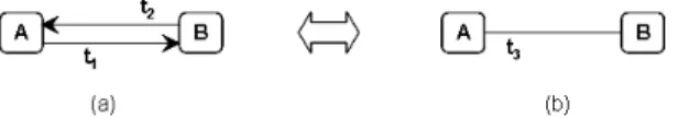
As we can observe in all of the three examples, biochemical reactions often proceed in both directions, with species A becoming species B and vice versa, normally with different rates. These reactions can be described with the following syntax:
[A] −→ [B]k1 (3) [B] −→ [A]k2
As we can see from the models in Figure 3, 4 and 5, modeling such bidirectional transformations with Petri nets requires introducing two tran-sitions, as shown in Figure 9. By applying the simplification we have in-troduced, the SPN in Figure 9 would be redrawn as the one in Figure 10, part (a). We can introduce a further simplification of notation by using non oriented arcs to represent the bi-directionality of the transformation, as shown in the same Figure 10, in part (b). Notice that we changed the tag associated to the arc to avoid any ambiguities. We shall use the more
2For instance, if n molecules of A are needed to generate m molecules of B – where n
and m are relatively prime with each other – a tag of the form n, m will be associated to the arc.
Figure 9: SPN for a bidirectional transition
Figure 10: Simplified model for reactions (3)
compact form shown in part (b) of Figure 10 to represent bidirectional re-actions whose rates are only dependent on the number of reactants through the mass-action law. We shall leave to the definition of the mapping between arcs and rates the task of specifying the two rates that are needed to get a fully defined stochastic model.
Let us now consider the more interesting case when a reaction is involving multiple reactants, the simplest form being the one described through the biochemical reaction syntax shown in formula (4).
[A] + [B]−→ [C]k (4) We have similar reactions in our examples, for instance in Figure 4, where the polymerase is binding to the σ32 factor. A classical Petri net model for
this reaction looks like the one shown in Figure 11. By applying the same
Figure 11: SPN model for reaction (4)
rationale of our transformation, we can simplify the SPN model in Figure 11 by removing the transition t1 and introducing a single direct hyperarc
going from A and B to C, as depicted in Figure 12, part (a). Similarly, a bidirectional reaction in which one molecule of C can decomplex back
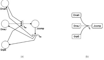
into one molecule of A and one molecule of B will be depicted with using a non oriented hyperarc connecting A and B boxes to the C box, as in Figure 12, part (b). It is worthwhile remarking that this graphical notation
Figure 12: Simplified models for reactions involving multiple reactants will reduce significantly the number of objects to be included in the model, making it much easier to draw and understand. For instance, consider the model of the biochemical reversible reaction for the σ32 pathway example, in which molecules of the three species DnaK, DnaJ and GrpE complex to form molecules of species Jcomp. We show in Figure 13 the original SPN model (a) and the simplified one (b) that would be obtained by using the notation defined in this paper. The simplified model has five elements, four
Figure 13: Comparison of original SPN and simplified models for the species and one hyperarc for the two reactions, whereas the original SPN one has 4 places, two transitions and eight direct arcs.
Consider now how to model thecreation of molecules of a species. This is of course a necessity to define proper boundaries to the biological phe-nomenon being modeled. Actually, molecules are not created, they just move
from an environment that is outside the scope of the model or are originated from a biochemical transformation that is not included in the model. The same applies to thedegradation processes, which make molecule disappear. For instance, in the model for theσ32 pathway we have represented the
re-sult of gene transcription and the degradation of mRNA molecules as input and output flows of tokens, entering and leaving the model. We will model these processes in our simplified notation as shown in Figure 14. We will
Figure 14: Creation and destruction processes
use the empty set symbol∅ symbol at the beginning of the arc (a) or at the end of the arc (b) to explicitly represent the fact that molecules are coming from or going to the outside of the model, respectively.
Let us now move to the most common case of biochemical transforma-tion involving chemical species which is favored, stimulated or catalyzed by another chemical species, which is however not changed in the reaction itself. A simple example of such reaction is one in which molecules of a chemical species A are transformed into molecules of species B with the intervention of molecules of species C. We have many examples in our modeled cases: MAPK being phosphorylated by active MAPKK, the σ32-Jcomp complex being degraded with the support of FtsH, CheY being deactivated by CheZ. In a standard SPN model, all the species involved in a reaction have to be linked to the transitions in which the species are involved. If the number of one of the species that participates in the reaction is not changed by the reaction, then the place that contains the tokens representing the molecules of that species will be both an input and an output place for the transition, as shown in Figure 15. This form of a reaction is not only the most common one, it is indeed a more precise way of modeling biological transformations. In fact, at a lower level of detail, very often biochemical transformations rely on molecular interaction to change one species into another. The majority of the arcs that we had to introduce in the SPN models of our examples are needed to account for this type of third-party molecular interaction. It can be argued that all species participating in a reaction will be changed by the reaction itself and that a model such as the one shown in Figure 15 is a very
Figure 15: SPN model of a catalysis reaction
abstract one. In fact, as described by the Michaelis-Menten dynamics of the reaction, an intermediate stage of the reaction exists, in which molecules of species CheY+P and CheY form a complex, they interact and then split to generate the two final molecules product of the reaction. However, the abstraction of the reaction described by the model in Figure 15 is commonly used in biology, primarily because the details of the Michaelis-Menten dy-namics are difficult to determine and not always known. At any rate, we shall keep in our simplified notation the possibility of modeling the reaction at both the levels of abstraction.
To simplify the notation shown in Figure 15, we will simply eliminate the loop of arcs that join place CheY to the transition modeling the traction, and shall put another tag with name of CheY on the arc representing the reaction, with also using a small arrow to indicate that CheZ is participating in the reaction, as shown in Figure 16. Notice that the model in Figure 15
Figure 16: Simplified model of a catalysis reaction
is telling us that species CheZ is involved in the reaction, but it is specifying anything about how the dynamics of the reaction is affected. We will leave this specification to the definition of the mapping between arcs and rates. The default will be to assume a classical mass-action law dynamics, i.e. in the form [CheY + P ] + [CheZ]−→ [CheY ]+[CheZ], but nothing prevent usk from allowing the CheY related rate of the transformation to be expressed by a generic function of the amount of tokens contained in placeCheY . Indeed,
the possibility of having generic marking-dependent functions in the tran-sition rates allows for introducing higher levels of abstractions in modeling biochemical reactions. Even if the details of the dynamics are not precisely known, it may still be feasible to determine by experiments of to postulate a concentration-dependent function that describes it. Whenever such de-scriptive function is available, it can be included into stochastic models as the ones we are considering here. It is worthwhile observing that, because of their usefulness in managing abstraction levels and making models more compact, generic marking dependencies are supported by many variants of SPNs, see for instance [6, 7].
We will allow also in the notation to represent, in quite a similar way, a negative effect of a biochemical species on the speed of the reaction, com-monly referred as a repression effect. We have not an examples of such repression in our examples, at least at the level of abstraction we selected for modeling the systems. Moreover, notice that a repression acting on a reaction is often indicative of a positive effect on the reverse reaction. How-ever, biologists often use in their notation the explicit representation of such a dependence in the dynamics of reactions, as we shall allow representing it as well in our formalism. We will represent the repression that a species X actuates on a reaction transforming A in B as shown in Figure 17, in which a tag is associated to arc representing the reaction and we use the arc ending with a bar to adhere to the biological notation. The semantics of the model
Figure 17: Simplified model of a catalysis reaction
shown in Figure 17 can be given in terms of an SPN only if the function of X that is actually expressing the intensity of the repression is taking values in the set 0, 1 and is non a non decreasing one. Indeed, in this case, there is an equivalent SPN that can model the repression through an inhibitory arc. In the more general (and interesting case), the semantics of the model can only be given in terms of an equivalent CTMC that has no counterpart in an SPN model (notice this only true for the specific class of SPNs we have been using in this paper, while more expressive SPN formalisms are able to handle this with marking-dependence features). Let us denote by
f (·) : N → R the function of the number of molecules of X that expresses the intensity of the repression, and let A0,B0 and X0 be initial number of molecules of species A, B and X, respectively. Then, the CTMC whose state space is the set E defined as follows:
E = {(i, j) | 0 ≤ i ≤ A0, B0 ≤ j ≤ A0+B0}
and whose entry kq~n, ~mk of the infinitesimal generator matrix Q, where ~n, ~m∈ E, is as follows: q~n, ~m= k∗· n1· f (X0) ifn1=m1+ 1∧ n2 =m2− 1 −k∗· n1· f (X0) if~n = ~m 0 otherwise
is the one equivalent to the model in Figure 17 and uniquely defines its semantics in terms of the evolution of the number of molecules over time from the initial state defined byA0,B0 and X0.
If multiple species are involved in a reaction, we will simply make the tag to be a list of all of them. Finally, we would like to observe that this modeling notation is pretty in line with the typical way biologists graphically describe the influence of a species X on a reaction between species Y and Z. This is indeed normally depicted with a direct arc coming from X into the arc linking Y and Z. We are proposing here a very similar graphical syntax, in which however just the final part of the arc is shown to avoid burdening models.
6
Simplifying the example models
In this section, we shall revise the SPN models of the biological examples defined in Section 4 and will apply the simplifications defined in Section 5. As we will see, the size of the models is greatly reduced and their readability improved. We shall comment on the results of such simplifications in next section.
6.1 MAPK model revisited
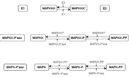
Figure 18 shows the MAPK cascade model, which has been obtained from the SPN model in Figure 3 by applying the simplifications proposed in Sec-tion 5. The model has 12 boxes, one for each biochemical species and 10 direct arcs, one for each reaction that can take place in the system. For the sake of simplicity, we are not associating tag names to the arcs.
Figure 18: Simplified MAPK model
Notice that we used a pair of direct arcs to model each of the five re-versible reaction, rather than using non oriented arcs. The reason is that the two side of the reaction have a dependence from two distinct chemical species (represented with the two small arcs and the tags), so this represen-tation is more informative that the one that uses a single non oriented arc and puts the two tags together.
It is also worthwhile observing that, by getting rid of useless arcs, this simplified model makes easier to understand that 4 out of the 12 biochem-ical species are not actually being changed by any transformation and that they can be removed from the model. Indeed, E1, E2, MAPKK-P’ase and MAPK-P’ase are indeed shown as isolated boxes. This means that what-ever type of function is used to express their influence on the reactions that modify the other species, the number of molecules of E1, E2, MAPKK-P’ase and MAPK-P’ase are playing into this function the role of constants rather than variables.
6.2 σ32 pathway model revisited
We show in Figure 19 the simplified model for the σ32 pathway. The new model has 12 boxes, the same number as the one of the places in the original SPN, but only 15 arcs and 2 hyperarcs, whereas the original SPN has 51 arcs and also 21 transitions. For the sake of simplicity, we are not associating tag names to the arcs.
Figure 19: Simplifiedσ32 pathway model
identifying the causality of events happening in the system, as it is easy to locate parts of it whose evolution starts only after some species are created. For instance, it is easy to understand that the mRNA transcription of the stress response proteins, which only starts afterσ32has been produced.
6.3 Chemotaxis model revisited
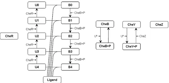
The SPN chemotaxis model provided in Figure 5 is dramatically reduced by the simplifications we propose in this paper. The 112 arcs of the SPN are reduced to 12 arcs and 5 hyperarcs in the simplified model and the 30 transitions of the SPN model do not appear anymore in the model in Figure 20. Notice that we have used the compact form U∗ to denote list of tags U0, U1, . . . , U4.
This example is indeed a very appropriate one to highlight the usefulness of explicit marking dependence in the models rather than representing it through arcs. In this particular case, the evolution of CheB and CheY is dependent on the marking of places U0, U1, . . . , U4. However, the function
that express such dependence is nothing else than the one given by the mass-action law. Indeed, the rate of the remass-action from CheB to CheB+P would be given by a functionf (·) : N5→ R defined as follows:
f (#CheB, #U0, #U1, #U2, #U3, #U4) =k∗· #CheB · 4
X
i=0
#Ui (5)
where #X denotes the number of molecules of species X and k∗ is the constant rate of the recation. Because in an SPN model such function is
Figure 20: Simplified chemotaxis model
not allowed, we need to split it into the 5 terms of the sum, and assign each term to a separate transition whose firing rate is defined according to the mass-action law. Consequently, we also need to add 4 arcs for each transition. With an explicit marking dependent function such as the one in formula (5), we can represent all of these arcs with a single one with the proper annotation.
7
Conclusions and future work
The simplifications we proposed in this paper are dealing with the graphical notation of a very popular modeling tool, which was first proposed in com-puter science to formally represent and analyze concurrent systems. The original Petri net variants did not account for time, which was added lately with the purpose of capturing the randomness of events occurrence times. A simple and mathematically tractable solution framework, provided by the theory of Markov chains, exists for stochastic Petri net models in which randomness is expressed through the negative exponential distribution of events occurrence times. Because of their graphical appeal, the existence of well-proved solution algorithms for their underlying stochastic processes, and the way they easily lend themselves to solution through simulation ap-proaches, the stochastic variants of Petri nets have been quite successful in various domains, including computer science, telecommunications, work-flow management, and more recently biology.
We proposed a simplification of the graphical formalism of SPNs, which aims at reducing the size of models by eliminating unnecessary graphical el-ements and at the same time including in models more expressive constructs that allow for expressing dependences of reaction dynamics from biochemical entities not modified in the reaction itself. The effectiveness of the simpli-fied notation in managing model conciseness has been demonstrated through the application to three case studies, for which a comparison between the SPN and the simplified models has been provided. Besides the significant reduction of the number of graphical elements contained in the model, the simplification we proposed also makes models more understandable as it helps highlighting the existing causality relations.
It is worthwhile comparing the objective of this paper with the recent proposals for the definition of a standardized graphical notation for systems biology, such as those ones put forward by the Systems Biology Graphical Notation (SBGN) international project [2]. The SBGN is still in a pro-posal phase, and a set of possible graphical notations are being compared to evaluate their respective merits and weaknesses. One difference between the approach we took and the SBGN proposals is related to the number of distinct modeling elements that are used to build the models. We propose to use only two graphical elements, namely boxes and hyperarcs, with the number of tokens being just an extra tag associated to places. Other ap-proaches being considered in the SGBN consider more graphical elements with specialized meanings, such as different form of boxes to represent com-pounds, arcs ending with various types of arrows to represent different types of dependences of reactions on biochemical species. We decided to take a minimalist approach to make models simpler to draw and more intuitive to understand, and our formalism can be also directly mapped into an existing modeling formalism with a formal semantics.
Because of its simplicity, it would be very easy to build a graphical user interface to support the editing of models based on the graphical formalism described in this paper. Moreover, because the semantics of the model is precisely described in terms of stochastic Petri nets and thus in terms of continuous time Markov chains, it will be also easy to create a layer of interpretation of the models into existing Gillespie-based simulators and Markov solution tools. These tasks will be the subject of our future work.
References
[2] http://www.sbgn.org.
[3] J. C. M. Baeten. A brief history of process algebra. Theoretical Com-puter Science, 335(2-3):131–146, 2005.
[4] David F. Blair. How bacteria sense and swim. Annual Review of Mi-crobiology, 49:498–522, 1995.
[5] Giovanni Chiola, Claude Dutheillet, Giuliana Franceschinis, and Serge Haddad. Stochastic well-formed colored nets and symmetric model-ing applications. IEEE Transactions on Computers, 42(11):1343–1360, 1993.
[6] Gianfranco Ciardo, Jogesh K. Muppala, and Kishor S. Trivedi. SPNP: Stochastic petri net package. In International Workshop on Petri Nets and Performance Models (PNPM’89), pages 142–151, 1989.
[7] Graham Clark, Tod Courtney, David Daly, Dan Deavours, Salem De-risavi, Jay M. Doyle, William H. Sanders, and Patrick Webster. The M¨obius modeling tool. In International Workshop on Petri Nets and Performance Models (PNPM’01), pages 241–250, Los Alamitos, CA, USA, 2001. IEEE Computer Society.
[8] J. Gamer, G. Multhaup, T. Tomoyasu, J. S. McCarty, S. R¨udiger, H. J. Sch¨onfeld, C. Schirra, H. Bujard, and B. Bukau. A cycle of binding and release of the DnaK, DnaJ and GrpE chaperones regulates activity of the Escherichia coli heat shock transcription factorσ32.EMBO Journal, 15(3):607–617, February 1996.
[9] Daniel Gillespie. Exact stochastic simulation of coupled chemical reac-tions. The Journal of Physical Chemistry, 81(25):2340–2361, 1977. [10] Peter J. E. Goss and Jean Peccoud. Quantitative modeling of stochastic
systems in molecular biology by using stochastic Petri nets.Proceedings of the The National Academy of Sciences, 95(12):6750–6755, June 1998. [11] David Harel. Statecharts: A visual formalism for complex systems.
Science of Computer Programming, 8(3):231–274, June 1987.
[12] Chi-Jing F. Huang and Ferrel James Jr. Ultrasensitivity in the mitogen-activated protein kinase cascade. Proceedings of the The National Academy of Sciences, 93(19):10078–10083, September 1996.
[13] Kurt Jensen. An introduction to the practical use of coloured petri nets. In W. Reisig and G. Rozenberg, editors, Lectures on Petri Nets II: Applications, volume 1492 of Lecture Notes in Computer Science, pages 237–292. Springer-Verlag, 1998.
[14] Marco Ajmone Marsan, Gianni Conte, and Gianfranco Balbo. A class of generalized stochastic Petri nets for the performance evaluation of mul-tiprocessor systems.ACM Transactions on Computer Systems, 2(2):93– 122, 1984.
[15] Hiroshi Matsuno, Yukiko Tanaka, Hitoshi Aoshima, Atsushi Doi, Mika Matsui, and Satoru Miyano. Using Petri net tools to study properties and dynamics of biological systems. In Silico Biology, 3(3):389–404, 2003.
[16] Torsten Nutsch, Dieter Oesterhelt, Ernst Dieter Gilles, and Wolfgang Marwan. A quantitative model of the switch cycle of an archaeal flagel-lar motor and its sensory control.Biophysical Journal, 89(4):2307–2323, October 2005.
[17] Mor Peleg, Daniel Rubin, and Russ B. Altman. Using Petri net tools to study properties and dynamics of biological systems. Journal of the American Medical Informatics Association, 12(2):181–199, 2005. [18] Wolfgang Reisig. Petri Nets: An Introduction, volume 4 of EATCS
Monographs in Theoretical Computer Science. Springer, 1985.
[19] R. Srivastava, M. S. Peterson, and W. E. Bentley. Stochastic kinetic analysis of Escherichia coli stress circuit using σ32 targeted antisense.
Biotechnology & Bioengineering, 75(1):120–129, October 2001.
[20] Dimitra Tsavachidou and Michael N. Liebman. Modeling and simu-lation of pathways in menopause. Journal of the American Medical Informatics Association, 9(5):461–471, 2002.
[21] Ranjith Vasireddy and Somenath Biswas. Modeling gene regulatory network in fission yeast cell cycle using hybrid Petri nets. In ICONIP - International Conference on Neural Information Processing, pages 1310–1315, 2004.