On the coupling of mechanics with bioelectricity and its role in morphogenesis

royalsocietypublishing.org/journal/rsif

Research

Cite this article: Leronni A, Bardella L,

Dorfmann L, Pietak A, Levin M. 2020 On the

coupling of mechanics with bioelectricity and

its role in morphogenesis. J. R. Soc. Interface

17: 20200177.

http://dx.doi.org/10.1098/rsif.2020.0177

Received: 16 March 2020

Accepted: 4 May 2020

Subject Category:

Life Sciences–Engineering interface

Subject Areas:

biophysics, biomechanics, bioengineering

Keywords:

bioelectricity, osmotic stress, electrostatic

stress, mechanical stress, mechanosensitive

ion channels, morphogenesis

Author for correspondence:

A. Leronni

e-mail: a.leronni@unibs.it

Electronic supplementary material is available

online at https://doi.org/10.6084/m9.figshare.

c.4977707.

On the coupling of mechanics

with bioelectricity and its role

in morphogenesis

A. Leronni

_{, L. Bardella}

_{, L. Dorfmann}

_{, A. Pietak}

_{and M. Levin}

1_{Department of Civil, Environmental, Architectural Engineering and Mathematics, University of Brescia,}

25123 Brescia, Italy

2_{Department of Civil and Environmental Engineering, Tufts University, Medford, MA 02155, USA} 3_{Department of Biomedical Engineering, Tufts University, Medford, MA 02155, USA}

4_{Allen Discovery Center, Tufts University, Medford, MA 02155, USA}

AL, 0000-0003-2134-9976; LB, 0000-0002-6042-0600; LD, 0000-0002-9665-0272; AP, 0000-0002-0246-0612; ML, 0000-0001-7292-8084

The role of endogenous bioelectricity in morphogenesis has recently been explored through the finite volume-based code BioElectric Tissue Simulation Engine. We extend this platform to electrostatic and osmotic forces due to bio-electrical ion fluxes, causing cell cluster deformation. We further account for mechanosensitive ion channels, which, gated by membrane tension, modulate ion fluxes and, ultimately, bioelectrical forces. We illustrate the potentialities of this combined model of actuation and sensing with reference to cancer progression, osmoregulation, symmetry breaking and long-range signalling. This suggests control strategies for the manipulation of cell networks in vivo.

1. Introduction

Traditionally, morphogenesis has been studied from a biochemical perspective. The pivotal contribution of Turing [1] proposes that chemical patterns generated through reaction and diffusion of chemical substances instruct embryo develop-ment. The work of Wolpert [2] suggests that the concentration gradient of morphogens provides positional information towards cell pattern formation.

However, as envisaged in [1], it is nowadays established that both biomecha-nical forces, including the osmotic pressure given by species concentrations, and bioelectricity, regulating the electrodiffusion of species, are fundamental in mor-phogenesis. Here, bioelectricity refers to signals generated by electrodiffusion of ions setting the voltage across the cell membrane (the membrane potential).

Bioelectrical signals in non-excitable cells influence formation and regulation of patterns [3–6]. In particular, Pietak & Levin [7] investigate the role of bioelectri-city in morphogenesis through the finite volume-based simulator BioElectric Tissue Simulation Engine (BETSE). By extending the BETSE platform to biochemi-cal regulatory networks, Pietak & Levin [8] model the dynamics by which the membrane potential controls, and is affected by, specific signalling chemicals on cellular and tissue-level scales. This approach has begun to identify interven-tions controlling complex morphogenesis of whole organs, such as repairing defects in a developing frog brain that would otherwise result from exposure to teratogens [9].

In BETSE, bioelectricity is described in terms of the evolution of electric potential and concentrations of ions across a cell network and its environment. Each cell communicates with the extracellular space through its membrane: passively, via voltage-gated or ligand-gated ion channels, and actively, via ion pumps. Moreover, cells passively exchange signals via voltage-gated gap junctions. Finally, passive transport occurs in the extracellular environment. Ion fluxes lead to membrane depolarization or hyperpolarization, that is, to increment or decrement of the membrane potential.

Along with electrical and chemical factors, force and stress fields play a role in morphogenesis [10–16]. However, in BETSE, cell mechanics has so far been

limited to a simplistic framework. Here, we explore the inter-play of electrostatic, osmotic and mechanical phenomena in biological cell clusters, inspired by recent theories coupling electrodiffusion and elasticity [17,18]. These have been fos-tered by the emergence of soft smart materials for sensing and actuation in robotics and biomedicine [19–21]. Specifi-cally, imbalance of charge and concentrations generates electrostatic and osmotic forces, impacting the mechanical behaviour of the cluster. By resorting to the soft robotics terminology, cells are actuated by endogenous bioelectricity.

Moreover, cells sense mechanical stimuli through several molecular structures [22]. Here, we account for mechanosensi-tive ion channels, whose activation depends on the membrane mechanics [23], where larger tension increases the opening probability [24]. This, in turn, alters transmembrane ion fluxes, and consequently the membrane potential. Ultimately, the latter qualifies both as an instructor and as a readout of the mechanical state of the cluster.

This investigation represents a first step towards a rigorous integration of bioelectricity with mechanobiology. Such integration has the potential to help understanding embryo-genesis, control of regeneration, and the transformation towards, or normalization of, cancer [25,26]. In the long term, unveiling the multiscale interconnections of electrostatic, osmotic and mechanical signals may be of great importance for the design of engineered living systems [27].

2. Bio-actuation: how bioelectrical forces shape

the multicellular mechanical response

We consider a cluster of closely packed cells, as depicted in figure 1. Ion channels allow for ion transport between the intra-cellular space and the thin extraintra-cellular space separating neighbouring cells. Ion fluxes also occur freely in the extracellu-lar space, which is connected to a global environment surrounding the cluster. Here, we focus only on the physical role of ions as carriers of charge and mass (thus disregarding any chemical processes) through the Nernst–Planck description of ion electrodiffusion [7].

We assume for the cluster mechanics a Cauchy continuum description, and neglect the thin extracellular space in evaluat-ing the electrostatic and osmotic forces exchanged by cells. Since the timescale associated with transport of ions is much

longer than that to achieve mechanical equilibrium [28], we neglect inertial effects in the linear momentum balance, which, in the absence of body forces, reads

r ! s ¼ 0, (2:1) where r! and σ denote divergence and total stress tensor (as · indicates single contraction product, such that (r ! s)j; sij,i).

In the framework for synthetic materials that inspired us [18] σreads

s ¼ smþ seþ so,

with σm, σeand σodenoting mechanical, electrostatic and osmotic

stresses, respectively.

In this first contribution on the interaction between bioe-lectricity and mechanobiology, we assume isotropic linear elasticity within a small deformation framework, such that the mechanical stress reads

sm¼ 2m1 þ l(tr 1)I, (2:2)

where μ = E/[2(1 + ν)] and λ = Eν/[(1 + ν) (1− 2ν)] are the Lamé parameters (with E the Young modulus and ν the Poisson ratio), tr denotes the trace operator, I is the second-order identity tensor and ε is the small strain tensor, which in turn is

1 ¼1₂[(ru) þ (ru)T], (2:3) with u denoting the displacement vector and (ru)ij; ui,jits

gradient. Henceforth, we consider spatially uniform elastic moduli, referring to the effective behaviour of closely packed cells of given cytoskeleton and anchoring junctions.

For an isotropic linear dielectric, the electrostatic (or Maxwell) stress reads [29]

se¼ 10 1rE $ E %1₂(E ! E)I

! "

,

in which⊗ indicates the tensor product (i.e. (E ⊗ E)ij≡ EiEj),

ε0 and εr are the vacuum and relative permittivities, and

E ¼ %rc is the electric field, with ψ denoting the electric potential. We consider the electrostatic stress across neigh-bouring membranes only, because elsewhere the electric field is irrelevant [7]. cytoskeleton anchoring junction cell extracellular space extracellular space mechanosensitive channel lipid bilayer intracellular space p n n r (b) (a)

Figure 1. Cell cluster (a) and equilibrium of a membrane patch (b).

roy

alsocietypublishing.org/journal/rsif

J.

R.

Soc.

Interfa

ce

17

:20200177

For suitably small ion concentrations, the osmotic stress is linear [28]:

so¼ %RTX i

(ci% c0i)I ; %RT(c % c0)I ; %poI, (2:4)

in which R is the gas constant, T is the absolute temperature, ciis the intracellular concentration of the ion species i and c is

the sum of intracellular ion concentrations (the osmotic concen-tration), with c0

i and c0their spatially uniform initial values;

finally, porepresents the osmotic pressure.

We disregard the explicit modelling of water flow allowed by aquaporins [30], whereby this is phenomenologically described by σo, which is, as σe, an active stress to be equilibrated

by σm through equation (2.1), thus coupling bioelectricity

and mechanics.

Under small strains, we compute the electrostatic and osmotic stresses in terms of membrane potential and ion con-centrations. Then, we introduce electrostatic and osmotic body forces fe¼ r ! se[29] and fo¼ r ! so, such that

f ¼ feþ fo¼ r ! (seþ so)

and equilibrium (2.1) becomes

r ! smþ f ¼ 0: (2:5)

By combining equations (2.2), (2.3) and (2.5), we obtain the following Cauchy–Navier equations:

r ! [mru þ m(ru)Tþ l(r ! u)I] þ f(E, c) ¼ 0: (2:6) We refer to the in-plane behaviour of a monolayer of cells, and assume that its mechanics is adequately described by either plane stress or plane strain states, whereby the real scenario lies in between. Hence, equation (2.6) consists of two coupled equations, to be solved in terms of f for the in-plane displacement components uxand uy.

Since electrodiffusion is time-dependent, f varies in time, leading to a time-varying mechanical response. We adopt a partly explicit time-integration scheme in which, at each step, we compute the displacement increment from equation (2.6) by evaluating f as a function of E and c at the beginning of the step; then, we employ the mechanical fields to update the bioelectrical fields at the following step, as illustrated in §3.

Equation (2.6) needs boundary conditions, which should be either kinematic

u ¼ !u on Su, (2:7)

with !u denoting the imposed displacement, or static tm; n ! sm¼ !tm on St, (2:8)

with !tm denoting the imposed mechanical traction.

In equations (2.7) and (2.8), Su and St are

complemen-tary parts of the total boundary S. In this investigation, we restrict attention to homogeneous mechanical boundary conditions, implying either !u ¼ 0 or !tm¼ 0, which are

suit-able for a cluster surrounded by a relatively stiff or compliant environment, respectively.

As detailed in the electronic supplementary material, to solve equation (2.6) we adopt the finite volume method, whereby each cell is discretized by a finite domain of regular hexagonal shape, and undergoes uniform displacements, strains and stresses.

3. Bio-sensing: how mechanosensitive ion

channels sense the cell membrane mechanics

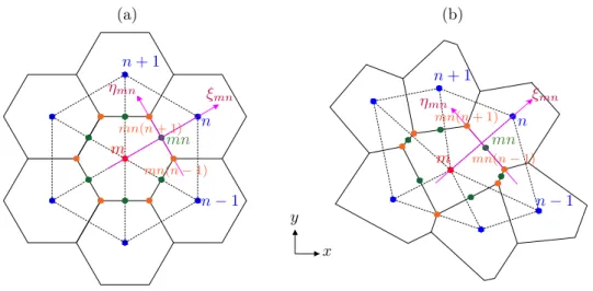
Mechanosensitive ion channels (MCs) respond to the mech-anics of the cell membrane [23]. Here, we assume that, for a given membrane mechanical state, MCs instantaneously reach their steady-state open probability. Moreover, as pro-posed by Wiggins & Phillips [24], we adopt the following energy form governing the MC behaviour:

G ¼1_{2 C}KU2

% nA, (3:1)

which depends on the hydrophobic mismatch 2U between chan-nel and membrane (figure 2) and on the membrane tension n; moreover, C ¼ 2pR and A ¼ pR2 _{are the circumference and}

area of the channel, whose radius is R, and K is the effective elas-tic modulus of the membrane, resulting from the hydrophobic mismatch linear elastic problem. As in figure 2, 2U = tm− W,

in which tmis the membrane thickness and W is the channel

hydrophobic length.

Wiggins & Phillips [24] consider the channel as a two-state system, which may be either closed, with radius RC,

or open, with radius RO. Hence, by expressing equation

(3.1) in terms of R and imposing G(RO) ¼ G(RC), the

opening membrane tension results nopen¼ KU 2

ROþ RC: (3:2)

The open state is energetically favoured when n > nopen. Then,

one resorts to the Boltzmann distribution for the channel

U W t_m

membrane

channel

Figure 2. Geometry of the channel–membrane system (adapted from Wiggins & Phillips [24]).

roy

alsocietypublishing.org/journal/rsif

J.

R.

Soc.

Interfa

ce

17

:20200177

open probability popen, increasing with n and being half if

n = nopen:

popen¼ 1

1 þ exp [p(R2

O% R2C)(nopen% n)=(kT)] , (3:3)

with k the Boltzmann constant.

In this work, we neglect interactions of neighbour MCs, thus assuming the following relation for the membrane diffusivity of the ion species i:

Di

mem¼ Dimem,0þ DiMCpopen(n), (3:4)

where Di

mem,0is the diffusivity in the absence of open MCs

and Di

MCis the additional diffusivity for all available

chan-nels open. The diffusivity Di

mem governs the transmembrane

electrodiffusion by entering the Goldman–Hodgkin–Katz flux equation, as implemented in BETSE [7].

We remark that MCs may exhibit an inactivated state [31,32], whose effect would impact our model by reducing the membrane diffusivity. Albeit relevant to quantitatively solve specific problems, accounting for this would not change the qualitative outcome of our investigation.

As bioelectricity influences biomechanics through the active stresses entering f in equation (2.6), biomechanics influences bioelectricity through MC gating. As already men-tioned, in our resolution strategy, we assume a simple partly explicit algorithm in which, at time t, we employ E and c to evaluate f. By choosing a suitably small time step Δt, solving equation (2.6) provides σm(t + Δt), which determines n as

follows, and finally Di

memthrough equations (3.3) and (3.4).

We treat the cell membrane as a structural membrane sub-ject to a pressure difference Δp, having principal curvature radii r1and r2. Equilibrium establishes that [10]

n ¼ Dp_rr1r2

1þ r2: (3:5)

In our framework, each cell experiences a uniform intracellu-lar mechanical pressure p = (tr σm)/3, while the extracellular

mechanical pressure vanishes, since the extracellular space is continuous and connected with the environment surrounding the cluster, and hence relatively free to accom-modate deformation. In the adopted small strains setting, balance equations are written on the undeformed configur-ation, such that r1 and r2 are the initial curvature radii.

Moreover, as illustrated in figure 1, to obtain an average mem-brane tension, we consider a cell of in-plane circular shape with radius r1= r, such that, the out-of-plane radius being

r2→∞, equation (3.5) particularizes to

n ¼ pr: (3:6)

The membrane equibiaxial tension state underlying equation (3.5) relies on the relatively small bending and shear stiffnesses of the membrane [10], the former conferred by the inner cytoskeleton and the surrounding glycocalyx, the latter resulting from the liquid-like behaviour of lipid molecules, freely flowing within the membrane surface. We remark that in patch clamp electrophysiology, used to investigate MC gating, equation (3.5) is also adopted to esti-mate n resulting from an applied pressure and a measured geometry [33]. This experimental technique circumvents known issues in singling out the tension felt by membranes in intact animal cells [34].

In the electronic supplementary material, we determine n on the basis of two richer models. First, we consider the case of plant cells, where the plasma membrane, in which MCs are embedded [32,35], is surrounded by a stiff cell wall, contributing to the mechanics of the cluster in place of the anchoring junctions. Second, back to the case of animal cells, we account for the through-the-thickness membrane stretch and for the transmembrane electric field; this analysis establishes the validity of equation (3.6).

4. Simulations

We consider four initial boundary-value problems relevant to morphogenesis. We limit our simulations to relatively short time intervals, such that the cluster evolution involves suitably small strains.

To simplify the interpretation of the results, we focus on a minimum number of ion species, that is, sodium ions Na+

and potassium ions K+_{, whose electrochemical potential}

gra-dients are directed outside and inside the cell, respectively. Depolarization of specific regions is triggered by increasing the membrane diffusivity to Na+_{, and hyperpolarization}

is obtained through K+_{-selective or cation non-selective}

chan-nels. Generic charge-balancing anions M− _{and fixed}

negatively charged proteins P− _{contribute as well to the}

membrane potential. Chloride ions could be considered for specific applications: accounting for their inflow would provide an osmotic effect qualitatively similar to Na+_{, along}

with a polarization effect similar to that due to the outflow of K+_{. Calcium is present at very small concentrations in}

cells and signals by virtue of its chemical nature: hence, it would not play a relevant role in our model.

As shown in [7], voltage-gated ion channels and gap junc-tions are involved in bioelectrical signalling. In the following, we provide only some comments about their possible quali-tative effect in our simulations, where we restrict attention to MCs, which are the most relevant when investigating the interplay between mechanics and bioelectricity.

4.1. Model parameters

The simulations are conducted at body temperature T = 310 K. Unless otherwise specified, we adopt the following model parameters.

We select a Young modulus E = 1.6 kPa, as obtained through indentation tests on healthy human cervical epithelial cells [36]. By assuming nearly incompressible material behav-iour, we set Poisson ratio ν = 0.49. As relative permittivity of the cell membrane we adopt εr= 3, as measured in [37].

The initial intracellular concentrations are: c0 Naþ ¼

10 mol m%3_{, c}0

Kþ¼ 140 mol m%3, c0P% ¼ 135 mol m%3 and

c0

M%¼ 15 mol m%3. The initial extracellular concentrations

are: c0

Naþ ¼ 145 mol m%3, c0_Kþ¼ 5 mol m%3, c0_P% ¼ 10 mol m%3

and c0

M%¼ 140 mol m%3. The adopted Na+ and K+

concen-trations are in the ranges of those found in physiological conditions in mammalian cells. Both inside and outside cells, the initial osmotic concentration is uniform and equal to c0₌

300 mol m−3_{, whereas the free charge r ¼ F}P

izici (with zi

denoting the valency of the ion i) is zero, corresponding to null active stresses. Hence, the initial configuration is unde-formed. Note that this does not correspond to physiological conditions, characterized by a resting membrane potential [7] and residual mechanical stresses [38].

roy

alsocietypublishing.org/journal/rsif

J.

R.

Soc.

Interfa

ce

17

:20200177

The diffusivity Di

mem,0of all mobile ions is 10−18m2s−1

[7], except for specific regions where we increase DNaþ

mem;0 as

a convenient way to trigger depolarization.

With reference to a MC of large conductance, we use RO¼ 3:5 nm and RC¼ 2:3 nm as open and closed radii

[24]. By considering a 1,2-dioleoyl-sn-glycero-3-phosphocholine lipid, abundant in lipid bilayers, the effective elastic modulus of the membrane and the hydrophobic mismatch are K = 27kT nm−3 and 2U =−0.4 nm, respectively [24]. Therefore,

the opening tension (3.2) results nopen= 0.19kT nm−2=

0.8 mN m−1, which agrees with experiments [39]. Finally, we adopt an in-plane cell radius r = 5 μm.

4.2. Simulation 1: cancer progression

We deal with a circular cluster of diameter of about 150 μm, composed of approximately 175 cells. We posit plane stress

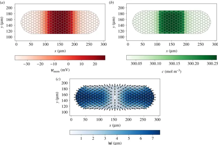
0 50 100 150 20 40 60 80 100 120 140 20 40 60 80 100 120 140 y ( mm) 20 40 60 80 100 120 140 20 40 60 80 100 120 140 y ( mm) 20 40 60 80 100 120 140 20 40 60 80 100 120 140 y ( mm) x (mm) 0 50 x (mm) 100 150 0 50 100 150 x (mm) 0 50 x (mm) 100 150 0 50 100 150 x (mm) 0 50 x (mm) 100 150 −20 0 20 40 ymem (mV) 300.1 300.2 300.3 c (mol m–3₎ 2 4 6 8 |f_e| (nN) |f_o| (nN) |u| (mm) 10 20 30 1 2 3 0 100 200 300 p (Pa ) (e) ( f ) (b) (a) (c) (d)

Figure 3. Membrane potential ψ

(x) (a), osmotic concentration c(x) (b), electrostatic force f

(x) (c), osmotic force f

(x) (d), displacement vector u(x) (e) and

mechanical pressure p(x) (f ) at t = 10 s. The central depolarized region, in which ions accumulate, is expanded by osmotic forces.

roy

alsocietypublishing.org/journal/rsif

J.

R.

Soc.

Interfa

ce

17

:20200177

state and, with reference to equation (2.7), we enforce !

u ¼ 0 on S ; Su.

We assume that a region of diameter of about 50 μm in the centre of the cluster consists of cancerous cells, which are typically characterized by a depolarized membrane potential [40]. This may be due to large intracellular Na+

level [41] and high expression of Na+_{channels [42]. To}

repro-duce this situation, we choose to increase DNa+

mem,0 in the

central region, thus therein setting DNa+

mem,0= 50 × 10−18m2s− 1_{. Owing to structural modifications of the cytoskeleton,}

can-cerous cells often appear softer than healthy ones [43]; thus, we adopt E = 1.4 kPa for them [36]. Figure 3 illustrates the results of the simulation at t = 10 s.

In the cancerous region, a depolarized membrane potential ψmemand an increased osmotic concentration c are originated

from the influx of Na+_{. The results show that ψ}

memreaches

the steady state in some milliseconds, while c continuously increases in the internal region during the simulation. Indeed, at steady-state membrane potential (as given by the Goldman–Hodgkin–Katz voltage equation) the net transmem-brane electric current is zero, while individual transmemtransmem-brane ion fluxes (as given by the Goldman–Hodgkin–Katz flux equation) are in general non-vanishing [7].

The depolarized region and the surrounding cluster attract each other by the electrostatic force fe. Simultaneously,

the strong gradient of c between the two regions generates a large outward osmotic force fo. An outward fo also arises at

the cluster boundary because of the difference in c between the boundary cells and the surrounding environment, the latter being progressively ion-depleted. Considering that fe

rapidly reaches a steady state, inspection of figure 3c,d suggests that osmotic stresses are more relevant than electro-static stresses in a long-lasting process as morphogenesis.

Due to the fofield, we register a large positive mechanical

pressure p in the cancerous region, and a smaller negative p in the healthy cells, compressed by the expansion of the tumour mass. The qualitative expansion of the inner region is inde-pendent of the mechanical boundary condition applied to the cluster, as this affects the qualitative deformation of the healthy cells, that would for instance expand if we applied !tm¼ 0 on S ; St.

To conclude, this simulation suggests that the depolarized state of cancerous cells may result in an osmotically driven expansion of the tumour, which is enhanced by their large compliance. Note that osmosis has already been related to cancer progression in the literature. Specifically, Stroka et al. [44] demonstrate that differential osmosis through the leading and trailing edges of a single tumour cell in a narrow channel promotes cell migration; Hui et al. [45] show that migration of individual cancer cells in a confined environment, driven by osmotic concentration gradients, is reduced by abating the concentration of aquaporins, suggesting that cancer progression might be hampered by reducing transmembrane osmosis.

Finally, we add that if gap junctions were accounted for, they would result in some transport of Na+_{from the inner region to}

the surrounding, that is, to a reduction of local depolarization accompanied with an increase of depolarized area.

4.3. Simulation 2: osmoregulation

We investigate the role of MCs as osmoregulators. We consider the same benchmark of Simulation 1, and additionally account

for either K+_{-selective MCs,}1 _{with D}Kþ

MC¼ 10%16m2s%1, or

cation non-selective MCs,2_{allowing transport of both K}+_and

Na+_{, with D}Kþ

MC¼ DNaMCþ¼ 10%16m2s%1. In figure 4, we

rep-resent ψmem(t), c(t) and p(t) for the innermost cell of the

cluster, comparing the responses obtained by accounting or not for MCs.

Without MCs, ψmem is nearly constant, whereas c and p

increase about linearly. With K+_{-selective MCs, when p, and}

hence the membrane tension, becomes sufficiently large, channels open, such that ψmem nonlinearly decreases and c

increases less than linearly, since the inflow of Na+_{due to the}

high DNaþ

mem competes with the outflow of K+ through MCs.

This effect hinders the increase of fo, such that, at the end of

the simulation, the value of p is about half of that in the absence of MCs. Given the selected diffusivities, we observe the same qualitative behaviour, though milder, in the case of cation non-selective MCs. 2 4 6 8 10 10 20 30 40 50 t (s) t (s) t (s) without MCs with K+ _{-sel. MCs}

with cation non-sel. MCs

2 4 6 8 10 2 4 6 8 10 300.0 300.1 300.2 300.3 300.4 _{without MCs} 100 200 300 400 p (P a) without MCs ymem (mV) c (mol m –3) with K+ _{-sel. MCs} with K+ _{-sel. MCs}

with cation non-sel. MCs

with cation non-sel. MCs

(b) (a)

(c)

Figure 4. Membrane potential ψ

(t) (a), osmotic concentration c(t) (b)

and mechanical pressure p(t) (c) in the innermost cell of the cluster. The

activation of MCs reduces ψ

and the increase rate of c and p.

roy

alsocietypublishing.org/journal/rsif

J.

R.

Soc.

Interfa

ce

17

:20200177

The foregoing negative feedback loop (where negative refers to the pressure reduction due to channel opening) represents a possible mechanism for cells to regulate osmotic pressure and, hence, their volume. Notably, MCs in bacteria, despite being non-selective to cations and anions [23], are hypoth-esized to operate as ‘safety valves’ to prevent the membrane failure when osmotic shock occurs [39]. The role of MCs as reg-ulators of cell volume in vertebrates is still debated, although several TRP channels exhibit osmosensitivity [34].

Furthermore, this simulation suggests that genetically modifying cells to induce a high expression of K+_-selective

MCs could help to restore the membrane potential of cancer-ous cells to its normal value, thereby hampering cancer progression. Importantly, Chernet & Levin [40] have shown that an artificial hyperpolarization obtained by overexpres-sing specific ion channels can inhibit tumour formation. Beside tumour cells, also embryonic and stem cells tend to be more depolarized than others [46], such that their activity could potentially be guided through the aforementioned control plans.

We finally note that accounting for voltage-gated K+

-selective or cation non--selective channels in place of the corre-sponding MCs would have the same qualitative effect on this benchmark, since pressurized regions are also depolarized.

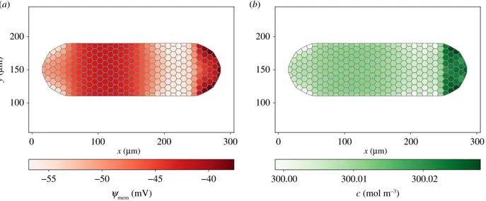
4.4. Simulation 3: symmetry breaking

In the ion flux model of left–right asymmetry [47], the asym-metric expression of K+ _{channels and H}+ _{pumps leads to}

ψmemdifferences between left and right sides of the embryo,

which in turn cause an asymmetric gene expression. Here,

we show that an asymmetric expression of K+_{-selective MCs}

can mechanically induce asymmetric patterning.

We consider the elongated cluster in figure 5, with major axis of about 300 μm along the x-direction and minor axis of about 100 μm along the y-direction, consisting of approximately 300 cells. Under plane stress, with reference to equations (2.7) and (2.8), we impose !u ¼ 0 on the straight top and bottom sides, along with !tm¼ 0 on the curved left and right boundaries.

In the central region V ¼ {100 , x , 200 mm, 8y} we set DNaþ

mem;0= 10−17m2s−1.

As shown in figure 5, ψmem and c are symmetric in the

absence of MCs, with V strongly depolarized for the influx of Na+_{. Osmotic forces at the boundary of V determine a}

horizontal symmetric elongation. If K+_{-selective MCs (with D}Kþ

MC¼ 10%16m2s−1) are present

only in the right half part of V, a local hyperpolarization occurs, as represented in figure 6. Eventually, the asymmetric expression of MCs is responsible of a ‘left–right asymmetry’ in the cell migration pattern: indeed, the vertical line corre-sponding to nil horizontal displacement is at the left of the mid-axis, and left side cells migrate slightly more than right side cells.

Figure 7 represents, as functions of t, the maxima of |ux|

at the left and right sides of the cluster, ul

x and urx,

respect-ively. After MCs activate, ul

x(t) becomes progressively larger

than ur

x(t), with both being reduced with respect to the case

without MCs.

In conclusion, differently from previous literature (see [47] and references therein), where left–right asymmetry of organs arises from asymmetric gene expression, here asymmetric pat-terning is originated by physical forces. In both cases, though, ion channels are fundamental in modulating the phenomenon. 0 50 100 150 200 250 300 0 50 100 150 200 250 300 100 120 140 160 180 200 −30 −20 −10 0 10 20 300.05 300.10 300.15 300.20 300.25 0 50 100 150 200 250 300 1 2 3 4 5 6 7 y ( mm) 100 120 140 160 180 200 y ( mm) 100 120 140 160 180 200 y ( mm) x (mm) x (mm) x (mm) |u| (mm) ymem (mV) c (mol m–3₎ (b) (a) (c)

Figure 5. Membrane potential ψ

(x) (a), osmotic concentration c(x) (b) and displacement vector u(x) (c) at t = 10 s, without MCs. The central depolarized

region, in which ions accumulate, determines a symmetric horizontal elongation of the cluster.

roy

alsocietypublishing.org/journal/rsif

J.

R.

Soc.

Interfa

ce

17

:20200177

Finally, we also argue that additional osmotically driven asymmetric morphogenesis should occur in the case of spatially non-uniform mechanical properties.

4.5. Simulation 4: long-range bioelectric signalling

Non-local bioelectrics (that is, the functional impact of the elec-trical state of cells at long distance from a morphogenetic event in vivo) is involved in tumorigenesis [48], brain patterning [49] and planarian regeneration [50]. Here, we explore whether and how long-range bioelectric signalling is mediated by cluster mechanics.

We deal with the same geometry of Simulation 3, but, under plane strain, we impose !u ¼ 0 on the curved left boundary, along with !tm¼ 0 on the rest of the boundary. In

the rightmost region of the domain Vr¼ {x . 250 mm, 8y}

we select DNa+

mem,0= 2 × 10−18m2s−1. We perform two 5 s

long analyses, one without MCs, and one with uniformly distributed K+_{-selective MCs featuring D}Kþ

MC¼ 10%17m2s%1.

Without MCs, as shown in figure 8,Vrappears depolarized.

The large gradient of c between Vr and the ion-depleted

environment produces large osmotic forces at the right end, determining a rightward expansion. The mechanical pressure field is non-trivial, being large in the depolarized region, redu-cing in the inner cluster region and then increasing again near the fixed left end.

As represented in figure 9, the MC opening produces a hyperpolarization of cells, which is larger near the curved boundaries, where p is larger. While in Simulations 2 and 3 the initial depolarization is reduced by the local opening of MCs, here MCs also open outside the depolarized region (that is, non-locally). This results in the hyperpolarization of the left end region, located far from the imposed bioelectrical perturbation. Note that, under plane stress, this long-range effect would be largely mitigated by the stress relaxation due to the free out-of-plane strain component.

To conclude, Simulation 4 highlights a possible case in which long-range bioelectric signalling, mediated by biome-chanical properties, occurs. Specifically, MCs-driven long-range signalling is most likely to be induced in cluster regions attracting larger mechanical stresses, thereby promoting MC opening. This may be due to specific mechanical boundary conditions or spatially variable mechanical properties. More-over, while in Simulations 2 and 3 MCs trigger a negative feedback loop by acting, respectively, as regulators of p (figure 4) and ux(figure 7), this simulation exhibits a positive

0 50 100 150 200 250 300 0 50 100 150 200 250 300 100 120 140 160 180 200 −30 −20 −10 0 10 20 300.025 300.050 300.075 300.100 300.125 300.150 300.175 300.200 300.225 0 50 100 150 200 250 300 1 2 3 4 5 6 7 y ( mm) 100 120 140 160 180 200 y ( mm) 100 120 140 160 180 200 y ( mm) x (mm) x (mm) x (mm) |u| (mm) ymem (mV) c (mol m–3₎ (b) (a) (c)

Figure 6. Membrane potential ψ

(x) (a), osmotic concentration c(x) (b) and displacement vector u(x) (c) at t = 10 s, with MCs. The asymmetric expression of

MCs determines a symmetry breaking in the migration pattern.

2 4 6 8 10 2 4 6 8 ur x ur x u1 x u1 x without MCs with MCs with MCs |ux | ( mm) t (s) ∫

Figure 7. Maxima of |u

| at the right and left sides of the cluster. They

pro-gressively diverge in time because of the asymmetric distribution of MCs.

roy

alsocietypublishing.org/journal/rsif

J.

R.

Soc.

Interfa

ce

17

:20200177

feedback loop, where the displacement field increases because of channel opening (figure 10). This is ultimately due to non-local signalling, and specifically to the emergence of a region, in the centre-left part of the cluster (figure 9), where ψmemis

larger, thereby producing further expansion forces.

5. Concluding remarks

The behaviour of bioelectric networks in tissues is complex; thus, the use of quantitative, bio-realistic simulators is essential to understand the dynamics of such signals and to infer interven-tions driving cellular systems to biomedically desirable states. The BioElectric Tissue Simulation Engine is a finite volume multi-physics simulator developed in [7] to model bioelectrical interactions in cell clusters, which we have here extended to

mechanics. On the one hand, the existence of electric fields and ion concentration gradients originates electrostatic and osmotic forces, which in turn, by equilibrium, lead to a mechanical stress field and, hence, to deformation. On the other hand, the mechanics of the cell membrane impacts the opening of ion channels, which are responsible for the transmembrane electrodiffusion, eventually modulating bioelectrical forces.

Our simulations show that osmotic forces induce an expan-sion of depolarized regions (such as tumour, embryonic and stem cell ensembles), while electrostatic forces are negligible. We suggest that overexpressing K+_{-selective MCs in}

depolar-ized cells could help to hinder cancer progression or to regulate the activity of embryonic and stem cells. Moreover, K+_{-selective MCs may be exploited to obtain asymmetric}

pat-terning, or to induce non-local bioelectric signals in regions

ymem (mV) c (mol m –3₎ 0 100 200 300 x (µm) 0 100 x (µm) 200 300 0 100 200 300 x (µm) 0 100 x (µm) 200 300 0 100 200 300 x (µm) 0 100 x (µm) 200 300 100 150 200 100 150 200 100 150 200 100 150 200 y (µm) 100 150 200 y (µm) 100 150 200 y (µm) −40 −35 −30 −25 −20 300.01 300.02 300.03 300.04 0 0.04 0.08 0.12 0 5 10 15 |f_o| (nN) |f_e| (nN) 0.5 1.0 1.5 2.0 |u| (µm) −100 0 100 200 300 p (Pa) (e) ( f ) (b) (a) (c) (d)

Figure 8. Membrane potential ψ

(x) (a), osmotic concentration c(x) (b), electrostatic force f

(x) (c), osmotic force f

(x) (d), displacement vector u(x) (e) and

mechanical pressure p(x) (f) at t = 5 s, without MCs. Osmotic forces at the right end produce a rightward elongation of the cluster and large mechanical pressure

near the fixed left end.

roy

alsocietypublishing.org/journal/rsif

J.

R.

Soc.

Interfa

ce

17

:20200177

with larger mechanical stress, as it may occur under specific constraints. Such constraints may even allow K+_-selective

MCs to trigger a positive feedback loop that amplifies the mech-anical response, while MCs usually establish negative feedback loops that regularize the global mechanical behaviour.

In this work, we have investigated a mechanism of mutual coupling between bioelectromechanical actuation and sensing, which may inspire the design of biological smart soft robots with physically integrated control structures [51,52]. However, relevant tasks should be accomplished to achieve this goal. On the experimental side, the suggested intervention strategies should be verified, by resorting to in vivo manipulation of ion channels through pharmacological or optogenetic techniques, and quantification of correspond-ing membrane potential variations, includcorrespond-ing long-range signalling. On the modelling side, the extension to large deformations is a crucial step for the following reasons.

First, finite deformations would permit the accurate inves-tigation of long-lasting morphogenetic events involving non-regular cell clusters. Moreover, finite deformations would allow modelling growth by introducing a suitable active strain contribution to the deformation gradient [53]. This would pro-vide insight on the mechanics of bioelectricity-driven regeneration, towards illustrating the ability of some biological systems to maintain a complex anatomical state despite drastic injury—a kind of homeostatic process [54]. Indeed, bioelectric

patterns and long-range signalling seem to be implicated in regeneration, as in planaria [50].

Furthermore, large deformations are necessary to intro-duce more appropriate mechanical constitutive laws, eventually accounting for the cell’s internal structure. For instance, the mechanics of the cytoskeleton could be described by leveraging on a statistical treatment of cross-linked polymers [55] or on a soft tensegrity structure model [56]. Lastly, large deformations would enable a more accurate evaluation of the cell membrane tension through the avail-ability of its local curvature on the deformed configuration.

Further ongoing work deals with osmotically driven water fluxes, both across the membrane via aquaporins [30] and freely in the extracellular space, by resorting to a poroelastic framework in which volumetric deformations depend on water flow [57].

Finally, the inclusion of voltage-gated ion channels, gap junc-tions and bio-actuation proteins, such as prestins (converting the membrane potential to force in the surrounding membrane [58]), would allow the investigation of further nonlinear feedback loops that might be exploited by cells in morphogenesis and fine-tuned in synthetic biology applications.

Data accessibility. The code mecBETSE developed within this

investi-gation is freely available at https://gitlab.com/betse/mecbetse.

Authors’ contributions.A.L. developed the theory, aided by L.B., L.D. and

A.P. A.L. extended the BETSE code under the guidance of A.P. and performed the numerical simulations; A.L. wrote the manuscript, aided by L.B. with relevant suggestions by M.L., A.P. and L.D. L.D., L.B. and M.L. supervised the project.

Competing interests.The authors declare no competing interests.

Funding.Work done within a research project financed by the Italian

Ministry of Education, University and Research (MIUR). The work of L.D. was supported in part by a Distinguished Visiting Fellowship awarded by the Royal Academy of Engineering, London, UK. M.L. gratefully acknowledges support by an Allen Discovery Center award from the Paul G. Allen Frontiers Group (12171).

Acknowledgements.L.D. acknowledges the Visiting Prof. appointment

provided by the University of Brescia.

Endnotes

1_K+_{-selective MCs are, for example, TREK and TRAAK channels,}

which can be found in eukaryotes [23].

2_{Cation non-selective MCs are, for example, the eukaryotic Piezo}

channels [31]. 0 100 200 300 100 150 200 100 150 200 −55 −50 −45 −40 300.00 300.01 300.02 y ( m m) x (mm) 0 100 x (mm) 200 300 ymem (mV) c (mol m–3) (b) (a)

Figure 9. Membrane potential ψ

(x) (a) and osmotic concentration c(x) (b) at t = 5 s, with MCs. These open because of the osmotic forces at the right end, and

trigger a change in ψ

near the fixed left end.

1 2 3 4 5 1 2 3 t (s) ux (m m) without MCs with MCs

Figure 10. Maximum of u

as a function of t. It increases more rapidly after

MCs activate.

roy

alsocietypublishing.org/journal/rsif

J.

R.

Soc.

Interfa

ce

17

:20200177

References

1. Turing AM. 1952 The chemical basis of morphogenesis. Phil. Trans. R. Soc. B 237, 37–72. (doi:10.1098/rstb.1952.0012)

2. Wolpert L. 1969 Positional information and the spatial pattern of cellular differentiation. J. Theor. Biol. 25, 1–47. (doi:10.1016/S0022-5193(69)80016-0)

3. McCaig CD, Rajnicek AM, Song B, Zhao M. 2005 Controlling cell behavior electrically: current views and future potential. Physiol. Rev. 85, 943–978. (doi:10.1152/physrev.00020.2004)

4. Bates E. 2015 Ion channels in development and cancer. Annu. Rev. Cell Dev. Biol. 31, 231–247. (doi:10.1146/annurev-cellbio-100814-125338) 5. Cervera J, Alcaraz A, Mafe S. 2016 Bioelectrical

signals and ion channels in the modeling of multicellular patterns and cancer biophysics. Sci. Rep. 6, 20403. (doi:10.1038/srep20403) 6. Levin M, Pezzulo G, Finkelstein JM. 2017

Endogenous bioelectric signaling networks: exploiting voltage gradients for control of growth and form. Annu. Rev. Biomed. Eng. 19, 353–387. (doi:10.1146/annurev-bioeng-071114-040647)

7. Pietak A, Levin M. 2016 Exploring instructive physiological signaling with the bioelectric tissue simulation engine. Front. Bioeng. Biotechnol. 4, 55. (doi:10.3389/fbioe.2016.00055)

8. Pietak A, Levin M. 2017 Bioelectric gene and reaction networks: computational modelling of genetic, biochemical and bioelectrical dynamics in pattern regulation. J. R. Soc. Interface 14, 20170425. (doi:10.1098/rsif.2017.0425)

9. Pai VP, Pietak A, Willocq V, Ye B, Shi N -Q, Levin M. 2018, HCN2 rescues brain defects by enforcing endogenous voltage pre-patterns. Nat. Commun. 9, 998. (doi:10.1038/s41467-018-03334-5)

10. Huang H, Kwon RY, Jacobs C. 2012 Introduction to cell mechanics and mechanobiology. New York, NY: Garland Science.

11. Mammoto T, Ingber DE. 2010 Mechanical control of tissue and organ development. Development 137, 1407–1420. (doi:10.1242/dev.024166)

12. Howard J, Grill SW, Bois JS. 2011 Turing’s next steps: the mechanochemical basis of morphogenesis. Nat. Rev. Mol. Cell Biol. 12, 392–398. (doi:10.1038/nrm3120)

13. Nelson CM, Gleghorn JP. 2012 Sculpting organs: mechanical regulation of tissue development. Annu. Rev. Biomed. Eng. 14, 129–154. (doi:10.1146/ annurev-bioeng-071811-150043)

14. Davidson LA. 2012 Epithelial machines that shape the embryo. Trends Cell Biol. 22, 82–87. (doi:10. 1016/j.tcb.2011.10.005)

15. Miller CJ, Davidson LA. 2013 The interplay between cell signalling and mechanics in developmental processes. Nat. Rev. Genet. 14, 733–744. (doi:10. 1038/nrg3513)

16. Kim Y, Hazar M, Vijayraghavan DS, Song J, Jackson TR, Joshi SD, Messner WC, Davidson LA, LeDuc PR.

2014 Mechanochemical actuators of embryonic epithelial contractility. Proc. Natl Acad. Sci. USA 111, 14 366–14 371. (doi:10.1073/pnas.1405209111) 17. Hong W, Zhao X, Suo Z. 2010 Large deformation

and electrochemistry of polyelectrolyte gels. J. Mech. Phys. Solids 58, 558–577. (doi:10.1016/j. jmps.2010.01.005)

18. Cha Y, Porfiri M. 2014 Mechanics and electrochemistry of ionic polymer metal composites. J. Mech. Phys. Solids 71, 156–178. (doi:10.1016/j.jmps.2014.07.006) 19. Trivedi D, Rahn CD, Kier WM, Walker ID. 2008 Soft

robotics: biological inspiration, state of the art, and future research. Appl. Bionics Biomech. 5, 99–117. (doi:10.1155/2008/520417)

20. Kim S, Laschi C, Trimmer B. 2013 Soft robotics: a bioinspired evolution in robotics. Trends Biotechnol. 31, 287–294. (doi:10.1016/j.tibtech.2013.03.002) 21. Rus D, Tolley MT. 2015 Design, fabrication and

control of soft robots. Nature 521, 467–475. (doi:10.1038/nature14543)

22. Ingber DE. 2006 Cellular mechanotransduction: putting all the pieces together again. FASEB J. 20, 811–827. (doi:10.1096/fj.05-5424rev)

23. Martinac B. 2004 Mechanosensitive ion channels: molecules of mechanotransduction. J. Cell Sci. 117, 2449–2460. (doi:10.1242/jcs.01232)

24. Wiggins P, Phillips R. 2004 Analytic models for mechanotransduction: gating a mechanosensitive channel. Proc. Natl Acad. Sci. USA 101, 4071–4076. (doi:10.1073/pnas.0307804101)

25. Chernet B, Levin M. 2013 Endogenous voltage potentials and the microenvironment: bioelectric signals that reveal, induce and normalize cancer. J. Clin. Exp. Oncol. S1. (10.4172/2324-9110.S1-002)

26. Mathews J, Levin M. 2018 The body electric 2.0: recent advances in developmental bioelectricity for regenerative and synthetic bioengineering. Curr. Opin. Biotech. 52, 134–144. (doi:10.1016/j.copbio. 2018.03.008)

27. Kamm RD et al. 2018 Perspective: the promise of multi-cellular engineered living systems. APL Bioeng. 2, 040901. (doi:10.1063/1.5038337) 28. Gurtin ME, Fried E, Anand L. 2010 The mechanics

and thermodynamics of continua. Cambridge, UK: Cambridge University Press.

29. Dorfmann L, Ogden RW. 2017 Nonlinear electroelasticity: material properties, continuum theory and applications. Proc. Math. Phys. Eng. Sci. 473, 20170311. (doi:10.1098/rspa.2017.0311) 30. Agre P. 2006 The aquaporin water channels. Proc.

Am. Thorac. Soc. 3, 5–13. (doi:10.1513/pats. 200510-109JH)

31. Coste B, Mathur J, Schmidt M, Earley TJ, Ranade S, Petrus MJ, Dubin AE, Patapoutian A. 2010 Piezo1 and Piezo2 are essential components of distinct mechanically activated cation channels. Science 330, 55–60. (doi:10.1126/science.1193270)

32. Peyronnet R, Tran D, Girault T, Frachisse J-M. 2014 Mechanosensitive channels: feeling tension in a

world under pressure. Front. Plant Sci. 5, 558. (doi:10.3389/fpls.2014.00558)

33. Haswell ES, Phillips R, Rees DC. 2011

Mechanosensitive channels: what can they do and how do they do it? Structure 19, 1356–1369. (doi:10.1016/j.str.2011.09.005)

34. Hoffmann EK, Lambert IH, Pedersen SF. 2009 Physiology of cell volume regulation in vertebrates. Physiol. Rev. 89, 193–277. (doi:10.1152/physrev. 00037.2007)

35. Hamilton ES, Schlegel AM, Haswell ES. 2015 United in diversity: mechanosensitive ion channels in plants. Annu. Rev. Plant Biol. 66, 113–137. (doi:10. 1146/annurev-arplant-043014-114700)

36. Guz N, Dokukin M, Kalaparthi V, Sokolov I. 2014 If cell mechanics can be described by elastic modulus: study of different models and probes used in indentation experiments. Biophys. J. 107, 564–575. (doi:10.1016/j.bpj.2014.06.033)

37. Gramse G, Dols-Pérez A, Edwards M, Fumagalli L, Gomila G. 2013 Nanoscale measurement of the dielectric constant of supported lipid bilayers in aqueous solutions with electrostatic force microscopy. Biophys. J. 104, 1257–1262. (doi:10. 1016/j.bpj.2013.02.011)

38. Lanir Y. 2009 Mechanisms of residual stress in soft tissues. J. Biomech. Eng. 131, 044506. (doi:10.1115/ 1.3049863)

39. Phillips R, Theriot J, Kondev J, Garcia H. 2012 Physical biology of the cell. New York, NY: Garland Science.

40. Chernet BT, Levin M. 2013 Transmembrane voltage potential is an essential cellular parameter for the detection and control of tumor development in a xenopus model. Dis. Model. Mech. 6, 595–607. (doi:10.1242/dmm.010835)

41. Yang M, Brackenbury WJ. 2013 Membrane potential and cancer progression. Front. Physiol. 4, 185. (doi:10.3389/fphys.2013.00185)

42. Djamgoz M. 2014 Biophysics of cancer: cellular excitability (‘celex’) hypothesis of metastasis. J. Clin. Exp. Oncol. S1, 005. (doi:10.4172/2324-9110.S1-005)

43. Lekka M. 2016 Discrimination between normal and cancerous cells using AFM. BioNanoScience 6, 65–80. (doi:10.1007/s12668-016-0191-3) 44. Stroka KM, Jiang H, Chen S -H, Tong Z, Wirtz D, Sun

SX, Konstantopoulos K. 2014 Water permeation drives tumor cell migration in confined microenvironments. Cell 157, 611–623. (doi:10. 1016/j.cell.2014.02.052)

45. Hui T et al. 2019 An electro-osmotic microfluidic system to characterize cancer cell migration under confinement. J. R. Soc. Interface 16, 20190062. (doi:10.1098/rsif.2019.0062)

46. Levin M. 2014 Molecular bioelectricity: how endogenous voltage potentials control cell behavior and instruct pattern regulation in vivo. Mol. Biol. Cell 25, 3835–3850. (doi:10.1091/mbc. e13-12-0708)

roy

alsocietypublishing.org/journal/rsif

J.

R.

Soc.

Interfa

ce

17

:20200177

47. Vandenberg LN, Levin M. 2013 A unified model for left–right asymmetry? Comparison and synthesis of molecular models of embryonic laterality. Dev. Biol. 379, 1–15. (doi:10.1016/j.ydbio.2013.03.021) 48. Chernet BT, Levin M. 2014 Transmembrane voltage

potential of somatic cells controls oncogene-mediated tumorigenesis at long-range. Oncotarget 5, 3287–3306. (doi:10.18632/oncotarget.1935) 49. Pai VP, Lemire JM, Chen Y, Lin G, Levin M.

2015 Local and long-range endogenous resting potential gradients antagonistically regulate apoptosis and proliferation in the embryonic CNS. Int. J. Dev. Biol. 59, 327–340. (doi:10.1387/ijdb. 150197ml)

50. Levin M, Pietak AM, Bischof J. 2019 Planarian regeneration as a model of anatomical homeostasis: recent progress in biophysical and computational

approaches. Semin. Cell Dev. Biol. 87, 125–144. (doi:10.1016/j.semcdb.2018.04.003).

51. Pfeifer R, Bongard J. 2006 How the body shapes the way we think: a new view of intelligence. Cambridge, MA: MIT Press.

52. Cheney N, Clune J, Lipson H. 2014 Evolved electrophysiological soft robots. In 14th Int. Conf. on Synthesis and Simulation of Living Systems, pp. 222–229. Cambridge, MA: MIT Press. (doi:10. 7551/978-0-262-32621-6-ch037)

53. Ambrosi D, Ben Amar M, Cyron CJ, DeSimone A, Goriely A, Humphrey JD, Kuhl E. 2019 Growth and remodelling of living tissues: perspectives, challenges and opportunities. J. R. Soc. Interface 16, 20190233. (doi:10.1098/rsif.2019.0233)

54. Pezzulo G, Levin M. 2016 Top-down models in biology: explanation and control of complex living

systems above the molecular level. J. R. Soc. Interface 13, 20160555. (doi:10.1098/rsif.2016.0555) 55. De Tommasi D, Puglisi G, Saccomandi G. 2015

Multiscale mechanics of macromolecular materials with unfolding domains. J. Mech. Phys. Solids 78, 154–172. (doi:10.1016/j.jmps. 2015.02.002)

56. Fraldi M, Palumbo S, Carotenuto AR, Cutolo A, Deseri L, Pugno N. 2019 Buckling soft tensegrities: fickle elasticity and configurational switching in living cells. J. Mech. Phys. Solids 124, 299–324. (doi:10.1016/j.jmps.2018.10.017)

57. Coussy O. 2004 Poromechanics. Hoboken, NJ: John Wiley & Sons.

58. Dallos P, Fakler B. 2002 Prestin, a new type of motor protein. Nat. Rev. Mol. Cell Biol. 3, 104–111. (doi:10.1038/nrm730)

roy

alsocietypublishing.org/journal/rsif

J.

R.

Soc.

Interfa

ce

17

:20200177

Supplementary Material:

On the coupling of mechanics with

bioelectricity and its role in morphogenesis

Journal of the Royal Society Interface

A. Leronni

, L. Bardella

, L. Dorfmann

, A. Pietak

, and M. Levin

Abstract

In this Supplementary Material, we focus on the finite volume discretization of the Cauchy-Navier equations governing the bioelectricity-driven mechanical response of the cell cluster. This is used to estimate the tension in the cell membranes, modulating the opening of mechanosensitive channels.

1

The finite volume discretization of the

Cauchy-Navier equations

The vectorial Cauchy-Navier equation describing the cluster mechanical response in terms of bioelectric fields reads

r ·⇥µ_{ru + µ(ru)}T _{+ (}

r · u)I⇤+ f (E, c) = 0 , (S1) in which _{r· denotes the divergence operator (with · denoting the single contraction} product),r denotes the gradient operator, I is the identity tensor, µ and are the Lam´e parameters, u is the displacement vector, and f is the body force, depending on the electric field E and osmotic concentration c. We discretize Eq. (S1) through the finite volume method [1, 2], by assuming that each biological cell occupies a finite domain of polygonal shape, and undergoes uniform displacements, strains, and stresses. Although in the simulations in the main article we consider a regular hexagonal grid, here we present a more generic discretization also suitable for an irregular grid. We remark

⇤_{Corresponding Author, email: a.leronni@unibs.it}

†_{Department of Civil, Environmental, Architectural Engineering and Mathematics, University of}

Brescia, 25123 Brescia, Italy

‡_{Department of Civil and Environmental Engineering, Tufts University, 02155 Medford MA, USA}

§_{Department of Biomedical Engineering, Tufts University, 02155 Medford MA, USA}

¶_{Allen Discovery Center, Tufts University, 02155 Medford MA, USA}

that cells are actually separated by thin extracellular spaces allowing transmembrane ion transport; however, we assume that a reliable overall mechanical response can be obtained by neglecting these extracellular spaces in solving Eq. (S1).

For a plane mechanical problem, Eq. (S1) is equivalent to the following system of equations: r ·hµrux+ µu,x+ ˜(r · u)i i + fx= 0 , (S2a) r ·hµ_ruy+ µu,y+ ˜(r · u)j i + fy= 0 , (S2b)

in which u,x⌘ @u/@x, u,y⌘ @u/@y, i is the unit vector in the x-direction, and j is the unit vector in the y-direction. Under plane strain conditions

˜ ⌘ = _{(1 + ⌫)(1}E⌫ _2⌫), whereas under plane stress conditions

˜ = E⌫ 1 ⌫2,

in which E is the Young modulus and ⌫ is the Poisson ratio.

1.1

Integral form of the Cauchy-Navier equations

We write Eqs. (S2) in integral form for each cell of the cluster. We refer to the generic cell m, with m = 1, ..., M and M the number of cells in the cluster. Upon applying the divergence theorem, we obtain

Z @Vm h µ_rux+ µu,x+ ˜(r · u)i i · n dA + Z Vm fxdV = 0 , (S3a) Z @Vm h µ_ruy+ µu,y+ ˜(r · u)j i · n dA + Z Vm fydV = 0 , (S3b) where Vm is the space region occupied by the cell m, @Vm is its boundary, and n is the outward unit normal to @Vm.

Since we model cells as polygons (in particular, as hexagons), the surface integrals in Eqs. (S3) can be split in the sum of the integrals over the cell faces:

Nm X n=1 Z @Vmn h µ(rux· nmn) + µ(u,x· nmn) + ˜(r · u)(i · nmn) i dA + Z Vm fxdV = 0 , Nm X n=1 Z @Vmn h µ(_ruy· nmn) + µ(u,y· nmn) + ˜(r · u)(j · nmn) i dA + Z Vm fydV = 0 , with Nm number of faces of the cell m, @Vm =SN_n=1m @Vmn, and @Vmn denoting the region occupied by the face n of the cell m, of area Amn and outward unit normal nmn (spatially uniform along each cell face). Note that, in this two-dimensional problem,

volume integrals become surface integrals, and surface integrals become line integrals, linearly weighed by the thickness along the z-direction.

1.2

Discretization

We now introduce appropriate numerical schemes to evaluate the integrals and the derivatives. By adopting the mid-point rule for the integrals, we obtain

Nm X n=1 h µ(_rux)mn· nmn+ µ(u,x)mn· nmn+ ˜(r · u)mn(i· nmn) i Amn+ fxmVm= 0 , Nm X n=1 h µ(_ruy)mn· nmn+ µ(u,y)mn· nmn+ ˜(r · u)mn(j· nmn) i Amn+ fymVm= 0 , where the superscript mn means “evaluated in the mid-point of the face n of the cell m”, whereas the superscript m means “evaluated in the center of the cell m”. More explicitly:

Nm

X n=1 ⇥

µ(umnx,xnmnx + umnx,ynmny ) + µ(umnx,xnmnx + umny,xnmny ) + ˜(umn x,xnmnx + umny,ynmnx ) ⇤ Amn+ fxmVm= 0 , Nm X n=1 ⇥

µ(umny,xnmnx + umny,ynmny ) + µ(umnx,ynmnx + umny,ynmny )

+ ˜(umnx,xnmny + umny,ynmny ) ⇤

Amn+ fymVm= 0 , and, after a convenient re-arrangement:

Nm

X n=1 h

(˜ + 2µ)umnx,xnmnx + µumnx,ynmny + µumny,xnmny + ˜umny,ynmnx i Amn+ fxmVm= 0 , (S4a) Nm X n=1 h

(˜ + 2µ)umny,ynmny + µumnx,ynmnx + µumny,xnmnx + ˜umnx,xnmny i

Amn+ fymVm= 0 . (S4b) To approximate the derivatives at mn, we resort to the local reference system ⇠mn, ⌘mn, represented for regular and non-regular grids in Fig. S1. This reference system is such that ⇠mnconnects the centers of the cells m and n, whereas ⌘mn is aligned with the face mn. The axis ⇠mnis directed from the cell m to the cell n and, by counterclockwise numbering the cells surrounding the cell m, the axis ⌘mnis directed from the cell n 1 to the cell n + 1, when there is no jump in numbering. We remark that, for a regular (hexagonal) grid, ⇠mnis normal to the face n, such that ⇠mnand ⌘mndefine an orthogonal

m mn n n + 1 n 1 mn(n + 1) mn(n 1) ⇠mn ⌘mn m mn n n + 1 n 1 mn(n + 1) mn(n 1) ⇠mn ⌘mn x y (a) (b)

Figure S1: Regular (a) and non-regular (b) grids with the local reference system ⇠mn, ⌘mn.

reference system. In general, this is not the case for a non-regular grid.

The derivatives of ui (with i = x, y) with respect to ⇠mnand ⌘mn can be expressed, through the chain rule, as follows:

2 6 4 umn i,⇠ umn i,⌘ 3 7 5 = 2 6 4 xmn ,⇠ y,⇠mn xmn ,⌘ y,⌘mn 3 7 5 | {z } Jmn 2 6 4 umn i,x umn i,y 3 7 5 ,

in which Jmn is the Jacobian matrix of the coordinate transformation. By inverting Jmn, we find the desired expressions for umn

i,x and umni,y: 2 6 4 umn i,x umn i,y 3 7 5 =_Jmn1 2 6 4 ymn ,⌘ ymn,⇠ xmn ,⌘ xmn,⇠ 3 7 5 2 6 4 umn i,⇠ umn i,⌘ 3 7 5 , (S5) where Jmn_{⌘ det J}mn = xmn

,⇠ ymn,⌘ xmn,⌘ ymn,⇠ . We approximate the metric quantities by

xmn,⇠ ⇡ xn _xm ⇠n _⇠m , y mn ,⇠ ⇡ yn _ym ⇠n _⇠m, (S6a) xmn,⌘ ⇡ xmn(n+1) _xmn(n 1) ⌘mn(n+1) _⌘mn(n 1) , y mn ,⌘ ⇡ ymn(n+1) _ymn(n 1) ⌘mn(n+1) _⌘mn(n 1), (S6b) where the superscripts mn(n + 1) and mn(n 1) indicate the vertexes in common among cells m, n, n + 1 and m, n, n 1 (see Fig. S1). In the case of a regular (hexagonal) grid, Jmndescribes the usual transformation rule for vector components between orthogonal reference systems, Eqs. (S6) are exact, and Jmn_{= 1. We approximate the displacement}

derivatives umn

i,⇠ and umni,⌘ through the central finite di↵erence scheme:

umni,⇠ ⇡ un i umi ⇠n _⇠m , (S7a) umni,⌘ ⇡ umn(n+1)_i umn(n 1)_i ⌘mn(n+1) _⌘mn(n 1). (S7b)

However, the displacement components in the vertexes are not the unknowns of the problem; hence, we approximate them through the average of the corresponding values in the surrounding cell centers:

umn(n+1)i ⇡ um i + uni + un+1i 3 , (S8a) umn(n 1)i ⇡ um i + uni + u n 1 i 3 . (S8b)

For a non-regular grid, the terms in Eqs. (S8) should be weighed through the relative distances between vertexes and centers. By substituting Eqs. (S8) into Eq. (S7b), we obtain

umni,⌘ ⇡

(un+1i un 1i )/3

⌘mn(n+1) _⌘mn(n 1). (S9)

Finally, by replacing Eqs. (S6), (S7a), and (S9) into Eq. (S5), we get umn i,x = (ymn(n+1) _ymn(n 1)_)(un i umi ) (yn ym)(u n+1 i u n 1 i )/3 (xn _xm_)(ymn(n+1) _ymn(n 1)_{) (y}n _ym_)(xmn(n+1) _xmn(n 1)₎, (S10a) umni,y = (xmn(n+1) _xmn(n 1)_)(un i umi ) + (xn xm)(un+1i u n 1 i )/3 (xn _xm_)(ymn(n+1) _ymn(n 1)_{) (y}n _ym_)(xmn(n+1) _xmn(n 1)₎, (S10b) where it is clear that in the approximation of the derivatives of the displacement components at mn also the cells n + 1 and n 1 are involved, even in the case of a regular grid. Substitution in Eqs. (S4) leads to

Nm X n=1 h (xn xm)(ymn(n+1) ymn(n 1)) (yn ym)(xmn(n+1) xmn(n 1))i 1 n (˜ + 2µ)⇥(ymn(n+1) ymn(n 1))(unx umx) (yn ym)(un+1x un 1x )/3 ⇤ nmnx +µ⇥ (xmn(n+1) xmn(n 1))(unx uxm) + (xn xm)(un+1x un 1x )/3 ⇤ nmny +µ⇥(ymn(n+1) ymn(n 1))(uny umy) (yn ym)(un+1y un 1y )/3 ⇤ nmny +˜⇥ (xmn(n+1) xmn(n 1))(uny uym) + (xn xm)(un+1y un 1y )/3 ⇤ nmnx o Amn + fxmVm⌘ Nm X n=1 HxmnAmn+ fxmVm= 0 , (S11a) 5

Nm X n=1 h (xn xm)(ymn(n+1) ymn(n 1)) (yn ym)(xmn(n+1) xmn(n 1))i 1 n (˜ + 2µ)⇥ (xmn(n+1) xmn(n 1))(uny uym) + (xn xm)(un+1y un 1y )/3 ⇤ nmny +µ⇥ (xmn(n+1) xmn(n 1))(unx uxm) + (xn xm)(un+1x un 1x )/3 ⇤ nmnx +µ⇥(ymn(n+1) ymn(n 1))(uny umy) (yn ym)(un+1y un 1y )/3 ⇤ nmnx +˜⇥(ymn(n+1) ymn(n 1))(unx umx) (yn ym)(un+1x un 1x )/3 ⇤ nmny o Amn + fymVm⌘ Nm X n=1 HymnAmn+ fymVm= 0 , (S11b) where we remind that nmn

x and nmny are the components of the normal unit vector directed from the cell m to the cell n, whereas Hmn

x and Hymn are the components of the numerical flux Hmn _{exchanged between the cells m and n [2], here physically} corresponding to a mechanical traction vector, and also depending on the unknowns in the cells n + 1 and n 1. Eqs. (S11) can be readjusted in a more convenient form, as follows: Nm X n=1 axxmnunx+ axymnuny + axxmmumx + axymmumy + fxmVm= 0 , (S12a) Nm X n=1 ayx mnunx+ ayymnuny + ayxmmumx + ayymmumy + fymVm= 0 , (S12b) where axxmn= (˜ + 2µ)(ymn(n+1) _ymn(n 1)_)nmn x µ(xmn(n+1) xmn(n 1))nmny (xn _xm_)(ymn(n+1) _ymn(n 1)_{) (y}n _ym_)(xmn(n+1) _xmn(n 1)₎Amn +1 3 (˜ + 2µ)(yn 1 _ym_)nm(n 1) x + µ(xn 1 xm)nm(n 1)y (xn 1 _xm_)(ymn(n 1) _ymn(n 2)_{) (y}n 1 _ym_)(xmn(n 1) _xmn(n 2)₎Am(n 1) +1 3 (˜ + 2µ)(yn+1 _ym_)nm(n+1) x µ(xn+1 xm)nm(n+1)y (xn+1 _xm_)(ymn(n+2) _ymn(n+1)_{) (y}n+1 _ym_)(xmn(n+2) _xmn(n+1)₎Am(n+1), axymn= µ(ymn(n+1) _ymn(n 1)_)nmn y ˜(xmn(n+1) xmn(n 1))nmnx (xn _xm_)(ymn(n+1) _ymn(n 1)_{) (y}n _ym_)(xmn(n+1) _xmn(n 1)₎Amn +1 3 µ(yn 1 _ym_)nm(n 1) y + ˜(xn 1 xm)nm(n 1)x (xn 1 _xm_)(ymn(n 1) _ymn(n 2)_{) (y}n 1 _ym_)(xmn(n 1) _xmn(n 2)₎Am(n 1) +1 3 µ(yn+1 _ym_)nm(n+1) y ˜(xn+1 xm)nm(n+1)x (xn+1 _xm_)(ymn(n+2) _ymn(n+1)_{) (y}n+1 _ym_)(xmn(n+2) _xmn(n+1)₎Am(n+1), axx mm= Nm X n=1 (˜ + 2µ)(ymn(n+1) _ymn(n 1)_)nmn x + µ(xmn(n+1) xmn(n 1))nmny (xn _xm_)(ymn(n+1) _ymn(n 1)_{) (y}n _ym_)(xmn(n+1) _xmn(n 1)₎Amn, 6

axymm= Nm X n=1 µ(ymn(n+1) _ymn(n 1)_)nmn y + ˜(xmn(n+1) xmn(n 1))nmnx (xn _xm_)(ymn(n+1) _ymn(n 1)_{) (y}n _ym_)(xmn(n+1) _xmn(n 1)₎Amn, ayxmn= µ(xmn(n+1) _xmn(n 1)_)nmn x + ˜(ymn(n+1) ymn(n 1))nmny (xn _xm_)(ymn(n+1) _ymn(n 1)_{) (y}n _ym_)(xmn(n+1) _xmn(n 1)₎Amn +1 3 µ(xn 1 _xm_)nm(n 1) x ˜(yn 1 ym)nm(n 1)y (xn 1 _xm_)(ymn(n 1) _ymn(n 2)_{) (y}n 1 _ym_)(xmn(n 1) _xmn(n 2)₎Am(n 1) +1 3 µ(xn+1 _xm_)nm(n+1) x + ˜(yn+1 ym)nm(n+1)y (xn+1 _xm_)(ymn(n+2) _ymn(n+1)_{) (y}n+1 _ym_)(xmn(n+2) _xmn(n+1)₎Am(n+1), ayymn= (˜ + 2µ)(xmn(n+1) _xmn(n 1)_)nmn y + µ(ymn(n+1) ymn(n 1))nmnx (xn _xm_)(ymn(n+1) _ymn(n 1)_{) (y}n _ym_)(xmn(n+1) _xmn(n 1)₎Amn +1 3 (˜ + 2µ)(xn 1 _xm_)nm(n 1) y µ(yn 1 ym)nm(n 1)x (xn 1 _xm_)(ymn(n 1) _ymn(n 2)_{) (y}n 1 _ym_)(xmn(n 1) _xmn(n 2)₎Am(n 1) +1 3 (˜ + 2µ)(xn+1 _xm_)nm(n+1) y + µ(yn+1 ym)nm(n+1)x (xn+1 _xm_)(ymn(n+2) _ymn(n+1)_{) (y}n+1 _ym_)(xmn(n+2) _xmn(n+1)₎Am(n+1), ayx mm= Nm X n=1 µ(xmn(n+1) _xmn(n 1)_)nmn x ˜(ymn(n+1) ymn(n 1))nmny (xn _xm_)(ymn(n+1) _ymn(n 1)_{) (y}n _ym_)(xmn(n+1) _xmn(n 1)₎Amn, ayymm= Nm X n=1 (˜ + 2µ)(xmn(n+1) _xmn(n 1)_)nmn y µ(ymn(n+1) ymn(n 1))nmnx (xn _xm_)(ymn(n+1) _ymn(n 1)_{) (y}n _ym_)(xmn(n+1) _xmn(n 1)₎Amn. We note that each coefficient axxmn, axymn, ayxmn, and ayymn is given by the sum of three contributions, whereby the first is associated with Hmn_{, the second with H}m(n 1)_{, and} the third with Hm(n+1)_{. Moreover, for the conservation of linear momentum for the cell} m, it can be shown that

Nm X n=1 axx mn+ axymn + axxmm+ axymm= 0 , Nm X n=1 ayxmn+ ayymn + ayxmm+ ayymm= 0 .

After writing Eqs. (S12) for each cell, we obtain a linear algebraic system of 2M equations of the type A u = b, where u is the unknown vector, containing the displace-ment components in the cell centers, b is the known vector, containing the body force components (due to electrostatic and osmotic stresses) in the cell centers, and A is the coefficient matrix, depending on the geometry and mechanical properties.

1.3

The coefficient matrix

We order the components of u and b as follows: uT =⇥u1x, u1y, ..., uMx , uMy

⇤ , bT = ⇥fx1V1, fy1V1, ..., fxMVM, fyMVM⇤, such that A is a block symmetric matrix:

A = 2 6 6 6 6 4 A11 A12 . . . A1M A12 A22 . . . A2M .. . ... . .. ... A1M A2M . . . AM M 3 7 7 7 7 5,

where, for m = 1, ..., M and n > m,

Amn= 2 6 4 axx mn axymn ayx mn ayymn 3 7 5

if the cell n adjoins the cell m, otherwise Amn= 0, and, for m = 1, ..., M ,

Amm= 2 6 4 axx mm axymm ayx mm ayymm 3 7 5 ⌘ X n6=m Amn. (S13)

We observe that the block symmetry of A originates because ⇠mn= ⇠nm, ⌘mn= ⌘nm, and nmn_{= n}nm_{, that is, because adjoining cells exchange equal and opposite fluxes:} Hmn

x = Hxnm, Hymn= Hynm; the matrices Amn and Ammare not symmetric; most of the Amnmatrices are zero matrices, and consequently A is sparse; because of Eq. (S13), deriving from the conservation of linear momentum for each cell, A is block diagonally dominant. The linear system can be solved by inverting the coefficient matrix: u = A 1b, once the boundary conditions are implemented.

1.4

The body force

Under small deformations, the body force can be computed once the coupled problems of electrostatics and ion transport are solved, that is, when the electric potential and ion concentrations are known in the cell cluster [3]. We write the discretized form of the body force by starting from

f =r · ( e+ o) ,

in which e is the electrostatic stress tensor

e= "0 

"rE⌦ E 1

2(E· E)I , (S14)

where⌦ indicates the tensor product, "0is the vacuum permittivity, and "ris the relative permittivity, whereas ois the osmotic stress tensor

o= RT (c c0)I , (S15)

where R is the gas constant, T is the absolute temperature, and c0_{is the reference value} of the osmotic concentration c. After integration, application of the divergence theorem, and split of the surface integral, we have

Z Vm f dV = Z Vm r·( e+ o) dV = Z @Vm n·( e+ o) dA = Nm X n=1 Z @Vmn nmn·( e+ o) dA .

By using the mid-point integration rule, we obtain Z Vm f dV ⇡ Nm X n=1 nmn· ( mn e + mno )Amn. (S16)

Upon substitution of Eqs. (S14) and (S15), Eq. (S16) becomes Z Vm f dV ⇡ "0 Nm X n=1 Amn 2 6 4 ⇥ ("r 1/2)(Exmn)2 1/2(Eymn)2 ⇤ nmn x + "rExmnEymnnmny "rExmnEymnnmnx + ⇥ ("r 1/2)(Eymn)2 1/2(Emnx )2 ⇤ nmn y 3 7 5 RT Nm X n=1 Amn(cmn c0) 2 6 4 nmn x nmn y 3 7 5 . (S17)

We assume the electric field across two cells to be normal to their interface, such that Emn

x = Emnnmnx , (S18a)

Eymn= Emnnmny , (S18b)

where Emn _{is computed through the central finite di↵erence scheme, as the di↵erence} between the membrane potentials of the neighboring cells divided by the double of the membrane thickness: Emn ⇡ n mem memm 2tm , (S19) 9