Simulation and optimization of supply chains and networks using a macroscopic approach

(1)

List of Figures

1.1 Conservation of ‡ux. . . 2

1.2 The characteristic for the Burgers equation in the (t; x)-plane. . . . 5

1.3 Superposition of characteristic curves for a Burgers equation. . . . 6

1.4 Solution to Burgers equation. . . 7

1.5 A solution u . . . 8

1.6 The condition (1.23) in the case u < u+. . . 10

1.7 The condition (1.23) in the case u > u+. . . 11

1.8 Shock and rarefaction curves. . . 16

1.9 Shock wave . . . 17

1.10 Rarefaction waves. . . 18

1.11 De…nition of ~f . . . 19

1.12 De…nition of . . . 19

1.13 Solution to the Riemann problem with u > 0 and u+ < (u). . . 20

1.14 A piecewise constant approximation of the initial datum satisfying (1.45) and (1.46). . . 25

1.15 The wave front tracking construction until …rst time of interaction. 26 1.16 Construction of “generalized tangent vectors”. . . 30

2.1 Example of a simple network structure . . . 43

2.2 Relation between ‡ow and density . . . 43

2.3 Geometry of a vertex with multiple incoming and outcoming arcs . 46 2.4 Supply network . . . 50

2.5 Flux (F): Left, f ( ; ). Right, f ( ; ). . . 52

2.6 A junction. . . 53

(4)

LIST OF FIGURES

2.8 Case ) . . . 58

2.9 Case ) . . . 58

2.10 An example of Riemann Solver: case ). . . 59

2.11 An example of Riemann Solver: case ). . . 60

2.12 Case ) for the Riemann Solver SC2. . . 64

2.13 Case ) for the Riemann Solver SC2. . . 64

2.14 Case ) and ) (namely 1) and 2)) for the Riemann Solver SC3. 66 2.15 One outgoing sub-chain. . . 68

2.16 P belongs to and P is outside . . . 69

2.17 One incoming sub-chain . . . 71

2.18 Waves production on an outgoing sub-chain: case a.2). . . 75

2.19 The outgoing sub-chain is an active constraint and the incoming ones are not active constraints. . . 76

2.20 The incoming sub-chains are active constraints and the outgoing one is not an active constraint. . . 77

3.1 Negative queue bu¤er occupancy at tn+1. . . 83

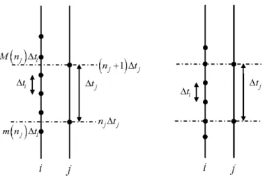
3.2 Case tj 1< tj. Left: not proportional case. Right: proportional case. . . 85

3.3 Case tj 1> tj: . . . 86

3.4 Di¤erent time meshes for ‡uxes corrections. . . 87

3.5 Case 1, with ₊; ₊ _{2 B. . . .} 95

3.6 Case 2, with ₊; ₊ _{2 A. . . .} 96

3.7 Intermediate state between the two waves. . . 96

4.1 In‡ow pro…le f1(t) prescribed as initial data on the …rst arc. . . . 101

4.2 Behaviour of queues . . . 102

4.3 Behaviour of …nal density . . . 102

4.4 Comparison between ordinary and other methods for q2. . . 103

4.5 Evolution of ‡ux f , density , and processing rate , on processors 2, 3, 4, with Riemann Solver SC1 and " = 0:1. . . 104

(5)

LIST OF FIGURES

4.7 Evolution of ‡ux f , density , and processing rate , on processors

2, 3, 4, with Riemann Solver SC3 and " = 0:1. . . 105

4.9 Supply chain network with 16 arcs and 10 nodes. . . 107

4.10 Queue on the last processor with 12= 0:7 and 12= 0:3. . . 108

4.11 Queue on the last processor with 12= 0:3 and 12= 0:7. . . 109

4.12 A Riemann Problem for the RA2-SC3 algorithm: the initial den-sity and the denden-sity after some times. . . 110

4.13 A Riemann Problem for the RA2-SC3 algorithm: the initial pro-duction rate and the propro-duction rate after some times. . . 110

4.14 A Riemann Problem for the SC2 algorithm: the initial density and the density after some times. . . 111

4.15 A Riemann Problem for the SC2 algorithm: the initial production rate and the production rate after some times. . . 111

4.16 aaaaa . . . 112

4.17 Results for Klar model. Case(a): density for the …rst processors; Case(b): density for the second processors; Case(c): density for the third processors. . . 113

4.18 Behaviour of the …nal density: ₁ for 0 x 10; t > 0, ₂ for 10 x 40; t > 0, and ₃; ₄; ₅ for 40 x 50; t > 0. . . 113

4.19 Results for the continuum-discrete model. Case(a): density for the …rst processors; Case(b): density for the second processors; Case(c): density for the third processors. . . 114

4.20 Behaviour of the …nal density: ₁ for 0 x 10; t > 0, ₂ for 10 x 40; t > 0, and ₃; ₄; ₅ for 40 x 50; t > 0. . . 115

4.21 Pro…le of input ‡ow with displacement of discontinuities . . . 115

4.22 j 1₂ < j 1₁ : . . . 117

4.23 j 1₂ > _j. . . 117

4.24 Shift of the queue j. . . 117

4.25 qj(t) > 0: . . . 118

4.26 Shift of the queue qj. . . 118

(6)

LIST OF FIGURES 4.28 qj(t) = 0: . . . 119 4.29 case 1). . . 120 4.30 case 2). . . 121 4.31 case 3). . . 122 4.32 case 4). . . 122

4.33 J versus Steepest Descent. . . 126

(7)

Introduction

The aim of this thesis is to present some macroscopic models for supply chains and networks able to reproduce the goods dynamics, successively to show, via sim-ulations, some phenomena appearing in planning and managing such systems and, …nally, to deal with optimization problems. The analyzed macroscopic models are based on the conservation laws, which are represented by special partial di¤erential equations where the variable is a conserved quantity, physically a quantity which can neither be created nor destroyed. The main idea is to look at large scales so to consider the processed parts as small particles which ‡ow in a continuous way and to assume the conservation of their density.

Depending on the observation scale supply networks modeling is characterized by di¤erent mathematical approaches: discrete event simulations and continuous models. Since discrete event models (see [11]) are based on considerations of individual parts, their main drawback is, however, an enormous computational e¤ort. Then a cost-e¤ective alternative to them is continuous models, described by some partial di¤erential equation. The …rst proposed continuous models date back to the early 60’s and started with the work of [4] and [15], but the most signi…cant in this direction was [10], where the authors, via a limit procedure on the number of parts and suppliers, have obtained a conservation law ([3], [9]), whose ‡ux involves either the parts density or the maximal productive capacity.

Then, in recent years continuous and homogenous product ‡ow models have been introduced, for example in [8], [14], [10], [17], [18], and they have been built in close connection to other transport problems like vehicular tra¢ c ‡ow and queuing theory. Extensions on networks have been also treated in [13], [19], [20].

In this thesis, starting by the historical model of Armbruster - Degond - Ring-hofer, we have compared two di¤erent macroscopic models, i.e. the Klar model,

(8)

Introduction

based on a di¤erential partial equation for density and an ordinary di¤erential equation to capture the evolution of queues, and a continuum-discrete model, formed by a conservation law for the density and an evolution equation for process-ing rate. Both the models can be applied for supply chains and networks.

A supply network is characterized by a set of interconnected suppliers which, in general, consist of a processor and, if we deal with the Klar model, a bu¤er or a queue. Each processor is characterized by a maximum processing rate _j, length Lj, and processing time Tj. The quantity L_Tj_j represents the processing

velocity. To study the dynamics at the connection points or junctions, some special parameters are introduced; in particular when the number of incoming suppliers is greater than the outgoing ones, we consider the priority parameters (q1; :::; qn),

where qi 2 ]0; 1[ determines a level of priority at the junction of incoming suppliers,

while, on the contrary, we consider the ‡ux distribution parameters ( 1; :::; m),

where j 2 ]0; 1[, with m

X

j=1

j = 1, indicates the percentage of parts addressed from

an incoming supplier to an outgoing one. At junctions, a way to solve Riemann problems, i.e. Cauchy problems with constant initial data on each arc, is prescribed for the continuum-discrete model and a solution at junctions guaranteeing the conservation of ‡uxes is de…ned.

We have to notice some di¤erences between the Klar and continuum-discrete model. In fact, the …rst one considers the formation and propagation of queue, under the assumption that the processing rate _j is constant, while the second one do not taking account of queues but describes the evolution of _j which is a time-spatial dependent function. It is evident that the two models complete each other. In fact, the approach of Klar is more suitable when the presence of queue with bu¤er is fundamental to manage goods production. On the other hand, the mixed continuum-discrete model is useful when there is the possibility to reorganize the supply chain, i.e when the productive capacity can be readapted for some contingent necessity. In order to make a comparison of the two models, some numerical results are shown via simulations.

Moreover, an optimization problem of sequential supply chains modeled by the Klar approach has been treated. The aim is to …nd the con…guration of production according to the supply demand minimizing the queues length, i.e. the costs of inventory, and obtaining an expected pre-assigned out‡ow. The control problem is

(9)

Introduction

solved introducing and minimizing a cost functional which takes into account the …nal ‡ux of production and the queues representing the stores. The functional is not linear, so to …nd its minimum, a mathematical technique has been introduced. It is based on the choice of an input ‡ow which is a piecewise constant function, with a …nite number of discontinuities. Considering on each of them an in…ni-tesimal displacement which generates traveling temporal shifts on processors and shifts on queues, we are able to compute numerically the value of the variation of functional respect to each discontinuities. Finally, we use the steepest-descent al-gorithm to …nd, via simulations, the optimal con…guration of input ‡ow, according to the pre-…xed desired production.

This work is organized as follow.

Chapter 1 deals with hyperbolic systems of conservation laws, introducing basic de…nitions and giving the tools to prove existence and uniqueness of solutions. Chapter 2 presents the main macroscopic models for supply chains and networks, based on conservation laws. Chapter 3 is devoted to numerical methods used to discretize the proposed models in Chapter 2. Chapter 4, …nally, compares, via simulations, the models for both chains and networks, and describes how to use the introduced optimization technique on Klar model to obtain a wished out‡ow minimizing the queues of the processed parts.

(10)

Chapter 1

Conservation Laws

In this chapter we present some basic de…nitions about system of conserva-tion laws which are special partial di¤erential equaconserva-tions where the variable is a conserved quantity. The models for supply chain networks we deal are based on conservation laws.

1.1 De…nitions

De…nition 1 A system of conservation laws in one space dimension is a system

of the form ₈ > > > > > < > > > > > : @tu1+ @xf1(u) = 0 : : @tun+ @xfn(u) = 0 (1.1) it can be written as @tu + @xf (u) = 0; (1.2)

where u = (u1; ::::un) : [0; +1[ R ! Rn is the “conserved quantity” and f =

(f1; ::::fn) : Rn! Rn is the ‡ux.

Remark 2 _{(The scalar case). If n = 1, u takes value in R and f : R ! R,} then (1.2) is a single equation. In this case, we say that (1.2) is a scalar equation.

(11)

De…nitions

Figure 1.1: Conservation of ‡ux.

d dt Z b a u (t; x) dx = Z b a f (u (t; x))_xdx = f (u (t; a)) f (u (t; b)) = = [in‡ow at a] [out‡ow at b]

holds. This relationship shows that the quantity u is neither created nor de-stroyed, i.e. in any interval [a; b] the total amount of u can change only due to the quantity of u entering and exiting respectively at x = a and x = b.

We always assume f to be smooth, thus, if u is a smooth function, then (1.2) can be rewritten in the quasi linear form

ut+ A (u) ux= 0; (1.3)

where A (u) is the Jacobian matrix of f at u.

De…nition 3 _{The system (1.3) is said “hyperbolic” if, for every u 2 R}n, all the eigenvalues of the matrix A (u) are real. Moreover (1.3) is said “ strictly hyper-bolic” if it is hyperbolic and if, for every u 2 Rn, the eigenvalues of the matrix A (u) are all distinct.

It is clear that equations (1.2) and (1.3) are completely equivalent for smooth solutions. Instead, if u has a jump, the (1.3) is in general not well de…ned, since there is a product of a discontinuous function A (u) with the distributional deriva-tive, which is in this case a Dirac measure. Hence (1.3) is meaningful only within a class of continuous functions.

(12)

De…nitions

non viscous gas take the form

t+ ( v)x= 0, (conservation of mass),

( v)_t+ v2_{+ p}

x = 0, (conservation of momentum),

( E)_t+ ( Ev + pv)_x = 0, (conservation of energy),

where is the mass density, v is the velocity while E = e + v₂2 is the energy density per unit mass. The system is closed by a constitutive relation of the form p = p ( ; e), giving the pressure as a function of the density and the internal energy. The particular form of p depends on what gas we consider.

A basic feature for the nonlinear system (1.2) is that the classical solutions may not exist for some positive time, even if the initial datum is smooth. This can be shown by the method of characteristics, brie‡y described for a quasilinear system. Consider the Cauchy problem

(

ut+ a (t; x; u) ux = h (t; x; u) ;

u (0; x) = u (x) ; (1.4)

and, for every y 2 R, the curves x (t; y), u (t; y) solving 8 > > > > > < > > > > > : dx dt = a (t; x; u) ; du dt = h (t; x; u) ; x (0; y) = y; u (0; y) = u (y) : (1.5)

The curves t ! x (t; y) when y 2 R are called characteristics. The implicit function theorem implies that the map

(t; y) ! (t; x (t; y)) (1.6)

is locally invertible in a neighborhood of (0; x0) and so it is possible to consider the

map u (t; x) = u (t; y (t; x)) where y (t; x) is the inverse of the second component of (1.6). It is easy to check that u (t; x) satis…es (1.4).

Example 5 Consider the scalar inviscid Burgers’ equation ut+

u2

(13)

De…nitions

with the initial condition

u (0; x) = u0(x) =

1

1 + x2: (1.8)

For t > 0 small, the solution can be found by the method of characteristics; if u is smooth, the (1.7) can be rewritten as

ut+ uux= 0;

from which we get that the directional derivative of the function u = u (t; x) along the vector (1; u) vanishes. Therefore the solution u to this Cauchy problem must be constant along the characteristic lines in the (t; x)-plane:

t ! (t; x + tu0(x)) = t; x +

t 1 + x2 :

For t < T = p8

27, these lines do not intersect together and so the solution is

classical u t; x + t 1 + x2 = 1 1 + x2: (1.9) Indeed, at t = p8

27, since the characteristics intersect together, a classical solution

cannot exist for t p8

27. In fact, the map

x ! x + t

1 + x2

is not one-to-one and (1.9) no longer de…nes a single valued solution of the Cauchy problem.

According to achieve a global existence result, we must deal with weak solu-tions.

De…nition 6 Fix u02 L1_loc(R; Rn) and T > 0. A function u : [0; T ] R ! Rn is

a weak solution to the Cauchy problem (

ut+ f (u)x = 0;

u (0; x) = u0(x) ;

(1.10)

if u is continuous as a function from [0; T ] into L1

loc and if, for every C1 function

with compact support contained in the set ] 1; T [ R, it holds Z T 0 Z Rfu t + f (u) _x_{g dxdt +} Z R u0(x) (0; x) dx = 0: (1.11)

(14)

De…nitions

Figure 1.2: The characteristic for the Burgers equation in the (t; x)-plane.

Remark 7 As consequence of the fact that u is continuous as a function from [0; T ] to L1

loc and of equation (1.11), we note that a weak solution u to (1.10)

satis…es

u (0; x) = u0(x) for a.e. x 2 R

Since weak solutions may develop discontinuities in …nite time, we introduce some notations to treat them.

De…nition 8 A function u = u (t; x) has an approximate jump discontinuity at the point ( ; ) if there exist vectors u , u+_{2 R}n and _{2 R such that}

lim r!0+ 1 r2 Z r r Z r rju ( + t; + x) U (t; x)j dxdt = 0; where U (t; x) = ( u ; if x < t; u+; if x > t: (1.12)

The function U is called a shock traveling wave. The following theorem holds.

Theorem 9 Consider a bounded weak solution u to (1.2) with an approximate jump discontinuity at ( ; ). Then

(15)

De…nitions

Figure 1.3: Superposition of characteristic curves for a Burgers equation.

Equation (1.13), called Rankine-Hugoniot condition, gives a condition on dis-continuities of weak solutions of (1.2) relating the right and left states with the “speed” of the “shock”. In fact considering the scalar case, (1.13) is a single equation and, for arbitrary u _{6= u}+, we have

= f (u

+₎ _{f (u )}

u+ _u ;

while for a n n system of conservation laws, (1.13) is a system of n scalar equations.

Example 10 Consider the Burgers equation ut+

u2

2 _x= 0 (1.14)

with the initial condition u0(x) =

(

1 _{jxj ; if x 2 [ 1; 1] ;}

0; otherwise: (1.15)

The corresponding characteristics are shown in Fig.1.3.Therefore for 0 t < 1, the function u (t; x) = 8 > > < > > : x+1 t+1; if 1 x < t; 1 x 1 t; if t < x < 1; 0; otherwise;

is a classical solution to 1.14. In this case the Rankine-Hugoniot condition reduces to = (u+₎2 2 (u )2 2 u+ _u = u++ u 2 :

(16)

Admissibility conditions

Figure 1.4: Solution to Burgers equation.

If t 1, then the function u (t; x) = ( _x+1 t+1; if 1 x 1 + p 2 + 2t; 0; otherwise;

satis…es the Rankine-Hugoniot condition at each point of discontinuity and so a weak solution to the Cauchy problem, given by (1.14) and (1.15), exists for each positive time (as shown in Fig.1.4).

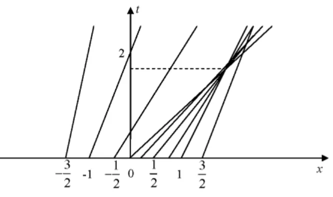
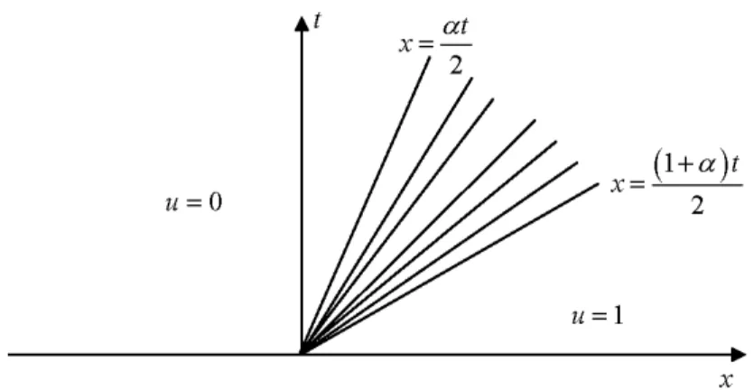
Example 11 Let the function u0 de…ned by

u0(x) :=

(

1; if x 0; 0; if x < 0:

For every 0 < _{< 1, the function u : [0; +1[} _{R ! R de…ned by}

u := 8 > > < > > : 0; if x < ₂t; ; if ₂t x < (1+ )t₂ ; 1; if x (1+ )t₂ ;

is a weak solution (shown in Fig.1.5) to the Burgers equation (1.14).

1.2 Admissibility conditions

As shown in the previous example, in presence of discontinuities, the de…nition of weak solution does not guarantee uniqueness to the Cauchy problem. Therefore, the notion of weak solution must be supplemented with admissibility conditions, motivated by physical considerations.

(17)

Figure 1.5: A solution u

1.2.1 Admissibility Condition 1

De…nition 12 (Vanishing viscosity) A weak solution u = u (t; x) to the Cauchy

problem ₍

ut+ f (u)_x = 0;

u (0; x) = u0(x) ;

(1.16) is admissible if there exists a sequence of smooth solutions u" to

u"_t + A (u") u"_x= "u"_xx (A = Df ) (1.17)

which converges to u in L1_Loc _{as " ! 0}+.

Unfortunately, it is very di¢ cult to provide uniform estimates to the parabolic system (1.17) and characterize the corresponding limits as " ! 0+. From the above condition, however, it can be deduced other conditions which can be more easily veri…ed in practice.

Now, arising from physical considerations, we introduce the entropy-admissibility condition.

De…nition 13 A C1 function _{: R}n _{! R is an entropy for (1.2) if it is convex} and there exists a C1 _{function q : R}n_{! R such that}

(18)

for every u 2 Rn_{. The function q is said an “entropy ‡ux” for . The pair ( ; q)}

is said “entropy-entropy ‡ux pair” for (1.2).

De…nition 14 (Entropy inequality) A weak solution u = u (t; x) to the Cauchy problem (1.16) is said entropy admissible if, for every C1 _{function '} _{0 with}

compact support in [0; T [ _{R and for every “entropy-entropy ‡ux pair” ( ; q), it}

holds _Z T 0 Z R ( (u) '_t+ q (u) '_x) dxdt 0 (1.19)

We consider now an entropy admissible solution u and a sequence of entropy-entropy ‡ux pairs ( ; q ) such that _! and q _{! q locally uniformly in} u 2 Rn_{. If '} _{0 is a C}1 _{function with compact support in [0; T [}

R, then Z T 0 Z R ( (u) '_t+ q (u) '_x) dxdt 0 (1.20)

for every _{2 N. Passing to the limit as} _{! +1 in (1.20), we obtain that} Z T

0

Z

R

( (u) '_t+ q (u) '_x) dxdt 0 (1.21)

From this, we can call a C0 function an entropy if there exists a sequence of entropies converging to locally uniformly. Moreover a C0 function q an entropy if there exists a sequence of entropies q , entropy ‡ux of , converging to q locally uniformly.

Remark 15 _{Consider the scalar Cauchy problem as in (1.16), where f : R ! R} is a C1 function. Then the relation between C1 entropy and entropy ‡ux is given by

0_{(u) f}0_{(u) = q}0_{(u) :} _(1.22)

Therefore if we take a C1 _entropy _{, every corresponding entropy ‡ux q has the}

following expression

q (u) = Z u

u0

0_{(s) f}0_{(s) ds;}

where u0 is an arbitrary element of R.

De…nition 16 A weak solution u = u (t; x) to the scalar Cauchy problem (1.16) satis…es the Kruzkov entropy admissibility condition if

Z T 0

Z

Rfju kj 't

(19)

Figure 1.6: The condition (1.23) in the case u < u+.

for every k 2 R and every C1 _{function '} _{0 with compact support in [0; T [} _R.

Theorem 17 Let u = u (t; x) be a piecewise C1 solution to the scalar equation (1.16). Then u satis…es the Kruzkov entropy admissible condition if and only if along every line of jump x = (t) the following condition holds. For every _{2 [0; 1]}

(

f ( u++ (1 ) u ) f (u+) + (1 ) f (u ) ; if u < u+;

f ( u+_{+ (1} _{) u )} _{f (u}+_{) + (1} _{) f (u ) ;} _{if u} _{> u}+_; (1.23)

where u := u (t; (t) ) and u+_{:= u (t; (t) +).}

The (1.23) implies that, if u < u+ (respectively u > u+) then the graph of f remains above (below) the segment connecting (u ; f (u )) to (u+; f (u+)) as shown in Fig.1.6 (Fig.1.7).

De…nition 18 (Lax Condition) A bounded weak solution u = u (t; x) to the Cauchy problem (1.16) is Lax admissible if, at every point of approximate jump, the speeds corresponding to the left and right states u , u+ satisfy

i u i u ; u+ i u+ (1.24)

(20)

Riemann Problem

Figure 1.7: The condition (1.23) in the case u > u+.

1.3 Riemann Problem

Let _Rn be an open set, let f : _{! R}n a smooth ‡ux and consider the system of conservation laws

ut+ f (u)x= 0; (1.25)

supposed to be strictly hyperbolic.

De…nition 19 A Riemann problem for the system (1.25) is the Cauchy problem for the initial datum ( Heaviside)

u0(x) =

(

u ; if x < 0;

u+; if x > 0; (1.26)

where u ; u+₂ _Rn.

To solve Cauchy problems, the solution of Riemann problem assumes a key role. In fact, to prove existence we use the wave-front tracking method consisting in the following steps:

1. approximate the initial condition with piecewise constant solutions; 2. at every point of discontinuity, solve the corresponding Riemann problem;

(21)

Riemann Problem

3. approximate the exact solution to Riemann problems with piecewise constant functions and piece them together to get a function de…ned until two wave fronts interact together;

4. repeat inductively the previous construction, starting from the interaction time;

5. prove that the functions so constructed converge to a limit function and prove that this limit function is an entropy admissible solution.

Denote by A (u) the Jacobian matrix of the ‡ux f and with 1(u) < < n(u) the n eigenvalues of the matrix A (u). For strictly hyperbolic systems, one

can …nd bases of right and left eigenvectors, fr1(u) ; ::::; rn(u)g and fl1(u) ; ::::; ln(u)g

depending strictly on u, such that

1. jri(u)j 1 for every u 2 and i 2 f1; :::; ng;

2. for every i; j 2 f1; :::; ng,

li rj :=

(

1; if i = j; 0; _{if i 6= j:}

We introduce the following notation. If i 2 f1; :::; ng, then the directional derivative of j(u) in the direction of ri(u) is given by

ri j(u) := lim "!0

j(u + "ri(u)) j(u)

" :

De…nition 20 _{We say that the i-characteristic …eld, i 2 f1; :::; ng, is genuinely} nonlinear if

ri i(u) 6= 0 8u 2 :

We say that the i-characteristic …eld, (i 2 f1; :::; ng) is linearly degenerate if ri i(u) = 0 8u 2 :

If the i-th characteristic …eld is genuinely nonlinear, then, for simplicity, we assume that ri i(u) > 0 for every u 2 .

(22)

Riemann Problem

1. Centered rarefaction waves. For u _{2 , i 2 f1; :::; ng and} > 0, we denote by Ri( ) (u ) the solution to

( _du

d = ri(u) ;

u (0) = u : (1.27)

Let > 0. De…ne u+ = Ri( ) (u ) for some i 2 f1; :::; ng. If the i-th

characteristic …eld is genuinely nonlinear, then the function

u (t; x) := 8 > > < > > : u ; if x < i(u ) t; Ri( ) (u ) ; if x = i(Ri( ) (u )) t; 2 [0; ] ; u+; if x > i(u+) t; (1.28)

is an entropy admissible solution to the Riemann problem ut+ f (u)x= 0;

u (0; x) = u0(x) ;

with u0de…ned in (1.26). The function u (t; x) is called a centered rarefaction

wave.

2. Shock waves. Fix u ₂ _{and i 2 f1; :::; ng. For some} 0, there exist smooth

functions Si(u ) = Si: [ 0; 0] ! and i: [ 0; 0] ! R such that:

(a) f (Si( )) f (u ) = i( ) (Si( ) u ) for every 2 [ 0; 0];

(b) dSi d 1; (c) Si(0) = u , i(0) = i(u ); (d) dSi( ) d j =0 = ri(u ); (e) d i( ) d j =0= 1 2ri i(u ); (f) d2Si( ) d 2 j =0 = 1 2ri ri(u ).

Let < 0. De…ne u+ = Si( ). If the i-th characteristic …eld is genuinely

nonlinear, then the function u (t; x) :=

(

u ; if x < i( ) t;

u+; if x > i( ) t;

(1.29) is an entropy admissible solution to the Riemann problem

(

ut+ f (u)x= 0;

u (0; x) = u0(x) ;

(23)

Riemann Problem

(a) Remark 21 If we consider < 0, then (1.29) is again a weak solution, but it does not satisfy the entropy condition.

3. Contact discontinuities. Fix u _{2 , i 2 f1; :::; ng and} _{2 [} 0; 0]. De…ne

u+ = Si( ). If the i-th characteristic …eld is linearly degenerate, then the

function u (t; x) := ( u ; if x < i(u ) t; u+; if x > i(u ) t; (1.30) is an entropy admissible solution to the Riemann problem

(

ut+ f (u)x= 0;

u (0; x) = u0(x) ;

with u0 de…ned in (1.26). The function u (t; x) is called a contact

disconti-nuity.

Remark 22 If the i-th characteristic …eld is linearly degenerate, then

i u = i u+ = i( )

for every _{2 [} 0; 0].

De…nition 23 The waves de…ned in (1.28), (1.29) and (1.30) are called waves of the i-th family.

For each _{2 R and i 2 f1; :::; ng, let us consider the function}

i( ) (u0) :=

(

Ri( ) (u0) ; if 0;

Si( ) (u0) ; if < 0;

(1.31) where u0 2 . The value is called the strength of the wave of the i-th

family, connecting u0 to i( ) (u0). It follows that i( ) (u0) is a smooth function.

Moreover let us consider the composite function

( 1; ::::; n) u := n( n) 1( 1) u ; (1.32)

where u ₂ and ( 1; ::::; n) belongs to a neighborhood of 0 in Rn. It is

possible to calculate the Jacobian matrix of the function and to prove that it is invertible in a neighborhood of (0; :::; 0). Hence we can apply the Implicit Function Theorem and prove the following result.

(24)

Riemann Problem

Theorem 24 For every compact set K , there exists > 0 such that, for every u _{2 K and for every u}+ ₂ _{with ju}+ _{u j} there exists a unique ( 1; ::::; n) in a neighborhood of 0 2 Rn satisfying

( 1; ::::; n) u = u+:

Moreover the Riemann problem connecting u with u+ has an entropy admissible solution, constructing by piecing together the solutions of n Riemann problems. Example 25 The 2 2 system of conservation laws

[u1]t+ u1 1 + u1+ u2 x = 0; [u2]t+ u2 1 + u1+ u2 x = 0; u1; u2 > 0: (1.33)

is justi…ed by the study of two components chromatography. Writing (1.33) in the quasi linear form (1.3), the eigenvalues and the eigenvectors of the corresponding 2 2 matrix A (u) are found to be

1(u) = _(1+u1 1+u2)2; 2(u) = 1 1+u1+u2; r1(u) = p_u1 1+u2 u1 u2 ! ; r2(u) = p1₂ 1 1 ! :

The …rst characteristic …eld is genuinely nonlinear, the second is linearly degener-ate. In this example, the two shock and rarefaction curves Si; Ri always coincide,

for i = 1; 2. Their computation is easy, because they are straight line (see Fig.1.8): R1( ) (u) = u + r1(u) ; R2( ) (u) = u + r2(u) : (1.34)

Observe that the integral curves of the two vector …elds r1 and r2 are respectively

the rays through the origin and the lines with slope 1. Now consider two states u = u₁; u₂ and u+ = u+₁; u+₂ . To solve the Riemann problem (1.26) for the system (1.25) we …rst compute an intermediate state u such that u = R1( ) (u ),

u+_{= R}

1( ) (u ) for some 1, 2. By (1.34), the components of u satisfy

u₁+ u₂= u+₁ + u+₂; u₁u₂ = u₁u₂:

The solution of the Riemann problem thus takes two di¤ erent forms, depending on the sign of = q u₁ 2+ u₂ 2 q (u₁)2+ (u₂)2:

(25)

Riemann Problem

Figure 1.8: Shock and rarefaction curves.

Case 1: 1 > 0. Then, the solution consists of centered rarefaction waves of the

…rst family and of a constant discontinuity of the second family:

u (t; x) = 8 > > > > > < > > > > > : u ; if x_t < 1(u ) ; su + (1 s) u ; if x_t = 1(su + (1 s) u ) ; u ; if 1(u ) < x_t < 2(u+) ; u+; if x_t 2(u+) ; (1.35) where s 2 [0; 1].

Case 2: 1 0. Then, the solution contains a compressive shock of the …rst family

(which vanishes if 1 = 0) and a contact discontinuity of the second family:

u (t; x) = 8 > > < > > : u ; if x_t < 1(u ; u ) ; u ; if 1(u ; u ) x_t < 2(u+) ; u ; if 1(u ) < x_t < 2(u+) ; (1.36)

Observe that 2(u ) = 2(u+) = (1 + u1+ u2) 1, because the second

characteris-tic …eld is linearly degenerate. In this special case since the integral curves of r1

are straight lines, the shock speed in (1.36) can be computed as

1 u ; u = Z 1 0 1 su + (1 s) u ds = = Z 1 0 1 + s (u₁+ u₂) + (1 s) u₁ + u₂ 2ds = = 1 (1 + u₁+ u₂) 1 + u₁ + u₂ :

(26)

Riemann Problem

Figure 1.9: Shock wave

1.3.1 The Non-Convex Scalar Case

Consider now the Riemann Problem (1.35)-(1.36) assuming f as uniformly convex function and G = (f0) 1.

Theorem 26 (Solution of Riemann’s problem)

If u > u+, the unique weak solution of the Riemann Problem is

u (t; x) = ( u ; x_t < ; u+; x_t > ; (1.37) where = f (u +₎ _{f (u )} u+ _u : (1.38)

If u < u+, the unique weak solution of the Riemann Problem is

u (t; x) = 8 > > < > > : u ; x_t < f0(u ) ; G x_t ; f0(u ) < x_t < f0(u+) ; u+; x_t > f0(u+) : (1.39)

Remark 27 In the …rst case the states u , u+ are separated by a shock wave with constant speed . In the second case the states u , u+are separated by a (centered) rarefaction wave.

Remark 28 Assume f is uniformly concave. In this case, if u > u+(respectively u < u+) the unique weak solution of the Riemann Problem is a rarefaction wave (a shock wave).

(27)

Riemann Problem

Figure 1.10: Rarefaction waves.

In the scalar case, the construction of solutions to Riemann problems can be done not only in the genuinely nonlinear case, i.e. for convex or concave ‡ux or linearly degenerate case, i.e. a¢ ne ‡ux.

Then, consider a scalar conservation law: ut+ f (u)x= 0;

with f : R ! R smooth. Given (u ; u+) the solution to the corresponding

Riemann problem is done in the following way.

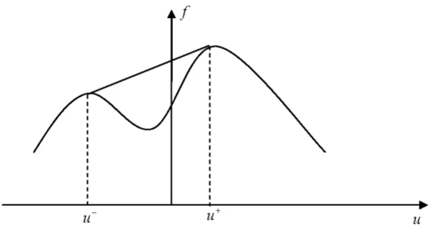
If u < u+ we let ~f be the largest convex function such that for every u 2

[u ; u+], it holds:

~

f (u) f (u);

If u > u+ we let ~f be the smallest concave function such that for every

u 2 [u+; u ], it holds:

~

f (u) f (u); Both the cases are shown in Fig.1.11.

Then the solution to the Riemann problem with data (u ; u+) is the solution

for the ‡ux ~f to the same Riemann problem. As we can see in this case, the ‡ux ~f is in general not strictly convex or concave but may contain some linear part. Then the solution to the corresponding Riemann problems may contain combinations of rarefactions and shocks.

(28)

Riemann Problem

Figure 1.11: De…nition of ~f .

Figure 1.12: De…nition of

For simplicity we will show the following special case. Fix the scalar conservation law:

ut+ (u3)x= 0;

and u > 0.

If u+ > u , then ~f coincides with f and the solution to the corresponding

Riemann problem is given by a single rarefaction wave.

If u+ < u , then we have to distinguish two cases. First, for every u de…ne

(u) u to be the point such that the secant from ( (u); f ( (u)) to (u; f (u)) is tangent to the graph of f (u) = u3 at (u) (Fig.1.12);

(29)

Functions with Bounded Variation

Figure 1.13: Solution to the Riemann problem with u > 0 and u+< (u).

In formulas: f (u) f ( (u)) u (u) = f 0_{( (u));} then u3 3(u) u (u) = 3 2_(u);

and one can easily get two solutions, i.e. the trivial one (u) = u and (u) =

u 2.

Now if u+ (u ) then again ~f coincides with f and the solution is given by

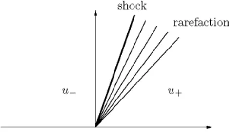
a single shock. Instead, if u+ < (u ), the solution to the Riemann problem is

given by the function:

u (t; x) = 8 > > < > > : u ; if x < 3₄u t; p_x 3t; if 3 4u t x 3(u+) 2_t; u+; if x > 3(u+)2t:

which is formed by a shock followed by a rarefaction attached to it, as shown in Fig.1.13.

In the case u < 0, the construction is symmetric with respect to the case u > 0, while for u = 0 the solution is always given by a rarefaction.

1.4 Functions with Bounded Variation

(30)

Functions with Bounded Variation

If we consider an interval J _{R and a function w : J ! R, the total variation} of w is de…ned by Tot.Var. w = sup 8 < : N X j=1 jw (xj) w (xj 1)j 9 = ;; (1.40)

where N 1, the points xj belong to J for every j 2 f0; : : : ; Ng and satisfy

x0 < x1 < < xN.

De…nition 29 _{We say that the function w : J ! R has bounded total variation if} Tot.Var. w < +1. We denote with BV (J) the set of all real functions w : J ! R with bounded total variation.

The total variation of a function w is a positive number. Moreover if w is a function with bounded total variation, this implies that it is a bounded function, but the converse is false. The following Lemma and Theorems show important properties of such functions.

Lemma 30 _{Let w : J ! R be a function with bounded total variation and x be a} point in the interior of J . Then, the limits

lim

x!x w(x); x!xlim+w(x)

exist. Moreover, the function w has at most countably many points of discontinuity. Theorem 31 (Helly) Consider a sequence of functions wn : J ! Rm. Assume

that there exist positive constants, C and M , such that: 1. Tot.Var. wn C for every n 2 N;

2. jwn(x)j M for every n 2 N and x 2 J.

Then there exist a function w : J ! Rm and a subsequence wnk such that

1. lim_k!+1wnk(x) = w(x) for every x 2 J;

2. Tot.Var. w C;

(31)

BV Functions in Rn

Theorem 32 Consider a sequence of functions wn : [0; +1[ J ! Rn. Assume

that there exist positive constants C, L and M such that: 1. Tot.Var. wn(t; ) C for every n 2 N and t 0;

2. jwn(t; x)j M for every n 2 N and x 2 J and t 0;

3. R_J_jwn(t; x) wn(s; x)j dx L jt sj for every n 2 N and t; s 0.

Then there exist a function w 2 L1

loc([0; +1 J ; Rn) and a subsequence wnk

such that

1. wnk ! w in L

1

loc([0; +1 J ; Rn) as k ! +1;

2. R_J_{jw (t; x)} _{w (s; x)j dx} _{L jt} _{sj for every t; s} 0.

Moreover the values of w can be uniquely determined by setting w(t; x) = lim

y!x+w(t; y)

for every t _{0 and x 2Int J. In this case we have} 1. Tot.Var. w(t; ) C for every t 0;

2. jw (t; x)j M for every x 2 J and t 0.

1.5 BV Functions in

_R

n

Now, we describe brie‡y the L1 theory for BV functions (CitaZion). Let be an open subset of Rnand consider w : _{! R. We denote with B( ) the -algebra} of Borel sets of _{and with B}c( ) the set

fB 2 B( ) : B compactly embedded in g : (1.41) De…nition 33 We say that _{: B}c( ) ! R is a Radon measure if it is countable

additive and _{(;) = 0. We denote with M( ) the set of all Radon measures on .} The following theorem holds.

(32)

BV Functions in Rn

Theorem 34 Fix a Radon measure _{2 M( ). There exist two positive and} unique Borel measures +; _{: B( ) ! [0; +1] such that}

(E) = +(E) (E) (1.42)

for every E 2 Bc( ).

De…nition 35 Fix a Radon measure _{2 M( ) and consider the total variation} of _{de…ned by juj :=} +₊ _{. We say that} _{has bounded total variation if}

juj ( ) < +1 and we denote with Mb( ) the set of all Radon measures with

bounded total variation.

Remark 36 Notice that Mb( ) is a Banach space with respect to the norm

jjujj

Mb( ) = juj ( ):

De…nition 37 We say that w : _{! R has bounded total variation if} 1. w 2 L1( );

2. the i-th partial derivative Diw exists in the sense of distributions and belongs

toMb( ), for every i = 1; : : : ; n.

The total variation of w is given by

n

X

i=1

jDiwj ( ):

We denote with BV ( ) the set of all functions de…ned on with bounded total variation.

Remark 38 The space BV ( ) is a Banach space with respect to the norm jjwjjL1_{( )}+

n

X

i=1

jDiwj ( ):

Remark 39 Let w 2 L1_{( ). Then w 2 BV ( ) if and only if there exists c 2}

(0; +1) such that _Z

w div 'dx c sup

x2 j' (x)j

for every ' 2 Cc1( ; Rn). In this case one can choose the constant c equal to the

(33)

Wave-Front Tracking and Existence of Solutions

Remark 40 If _{is an interval of R, then the two descriptions of BV functions} are not completely equivalent. The most important di¤ erence is that if we change the values of a BV function w in a …nite set, then the total variation of w changes but remain …nite if we consider the …rst description, while it does not vary in the second case. Therefore, if we are interested only in the L1 equivalence class, then we can assume that a BV function w is right continuous or left continuous.

1.6 Wave-Front Tracking and Existence of Solutions

This section deals with the existence of an entropy admissible solution to the

Cauchy problem ₍

ut+ [f (u)]x = 0;

u(0; ) = u( ); (1.43)

where f : Rn ! Rn is a smooth ‡ux and u 2 L1(Rn) is bounded in total variation. In order to prove existence, we construct a sequence of approximate solutions using the method called wave-front tracking algorithm.

We start considering the scalar case, while, for the system case, we will give some references.

1.6.1 The Scalar Case

We assume the following conditions: (C1) _{f : R ! R is a scalar smooth function;}

(C2) the characteristic …eld is either genuinely nonlinear or linearly degenerate. The construction starts at time t = 0 by choosing a sequence of piecewise constant approximations (u ) of u such that

Tot.Var. fuvg Tot.Var. fug ; (1.44)

jjuvjj_L1 jjujj_L1 (1.45)

(34)

Figure 1.14: A piecewise constant approximation of the initial datum satisfying (1.45) and (1.46).

jjuv ujjL1 <

1

; (1.46)

for every _{2 N (see Fig.1.14).}

Fix _{2 N. By (1.44), u}v has a …nite number of discontinuities, say x1 <

< xN. For each i = 1; : : : ; N , we approximately solve the Riemann Problem

generated by the jump (u (xi ); u (xi+)) with piecewise constant functions of

the type '(x xi

t ), where ' : R ! R. More precisely, if the Riemann Problem

generated by (u (xi ); u (xi+)) admits an exact solution containing just shocks

or contact discontinuities, then '(x xi

t ) is the exact solution, while if a rarefaction

wave appears, then we split it in a centered rarefaction fan, containing a sequence of jumps of size at most 1, traveling with a speed between the characteristic speeds of the states connected. In this way, we are able to construct an approximate solution u (t; x) until a time t1, where at least two wave fronts interact together

(see Fig.1.15).

Remark 41 In the scalar case, if the characteristic …eld is linearly degenerate, then all the waves are contact discontinuities and travel at the same speed. There-fore, the previous construction can be done for every positive time.

Remark 42 Notice that it is possible to avoid that three of more wave fronts interact together at the same time slightly changing the speed of some wave fronts. This may introduce a small error of the approximate solution with respect to the exact one.

(35)

Figure 1.15: The wave front tracking construction until …rst time of interaction.

At time t = t1, u (t1; ) is clearly a piecewise constant function. So we can

repeat the previous construction until a second interaction time t = t2 and so on.

In order to prove that a wave-front tracking approximate solution exists for every t 2 [0; T ], where T may be also +1, we need to estimate

1. the number of waves;

2. the number of interactions between waves; 3. the total variation of the approximate solution.

The …rst two estimates are concerned with the possibility to construct a piece-wise constant approximate solution. The third estimate, instead, is concerned with the convergence of the approximate solutions towards an exact solution.

Remark 43 The two …rst bounds are nontrivial for the vector case and it is nec-essary to introduce simpli…ed solutions to Riemann problems and/or non-physical waves.

The next lemma shows that the number of interactions is …nite.

Lemma 44 The number of wave fronts for the approximate solution u is not increasing with respect to the time and so u is de…ned for every t 0. Moreover the number of interactions between waves is bounded by the number of wave fronts. Lemma 45 The total variation of u (t; ) is not increasing with respect the time. Therefore for each t 0

(36)

The following theorem holds.

Theorem 46 _{Let f : R ! R be smooth and u 2 L}1_{(R) with bounded variation.} Then there exists an entropy-admissible solution u(t; x) to the Cauchy problem (1.43) de…ned for every t 0. Moreover,

jju (t; )jjL1 jju ( )jjL1 (1.48)

for every t 0.

1.6.2 The System Case

For systems, since more types of interaction may happen, the construction of wave-front tracking approximations is more complex. In particular the bounds on number of waves, interactions and BV norms are no more directly obtained.

In this case, in order to show the basic ideas for obtaining the needed bounds, we start giving some total variations estimates for interaction of waves along a wave-front tracking approximation.

The constants in the estimates depend on the total variation of the initial datum, which is assumed to be su¢ ciently small.

Consider a wave of the i-th family of strength i, i 6= j, and indicate by 0_k

(k 2 f1; :::; ng) the strengths of the new waves produced by the interaction. Then it holds i 0i + j 0j + X k6=i;j 0 k C j ij j jj ; (1.49)

For the case i = j, let us indicate by i;1and i;2the strengths of the interacting

waves, then it holds

i;1+ i;2 0i +

X

k6=i 0

k C j i;1j j i;2j : (1.50)

It is possible now, …xing a parameter v, to split rarefactions in rarefaction

fans with shocks of strength at most v. Also, only if the product of interacting

waves is bigger than v, at each interaction time, the new Riemann Problem can

be exactly solved eventually splitting the rarefaction waves in rarefaction fans. Otherwise, the Riemann Problem is only solved with waves of the same families

(37)

of the interacting ones, the error being transported along a non-physical wave, traveling at a speed bigger than all waves. In this way, it is possible to control the number of waves and interactions and then let v go to zero [6].

Consider now a wave-front tracking approximate solution uv and let x (t),

of family i and strength , indicate the discontinuities of uv(t). We say two

discontinuities are interacting if x < x and either i > i or i = i and at least one of the two waves is a shock. De…ne the Glimm functional computed at uv(t)

as:

Y (uv(t)) = Tot.Var. (uv(t)) + C1Q (uv(t)) ;

where C1 is a constant to be chosen suitably and

Q (uv(t)) =

X

j j j j

where the sum is over interacting waves. It can be proved that Y is equivalent to the functional measuring the total variation. Clearly such functional changes only at interaction times.

Using the interaction estimates (1.49) and (1.50), at an interaction time t, we get

jTot.Var. (uv(t+)) Tot.Var. (uv(t ))j C j ij j jj ;

Q (uv(t+)) Q (uv(t )) C1j ij j jj + C j ij j jj Tot.Var. (uv(t )) :

Therefore

Y (uv(t+)) Y (uv(t )) j ij j jj [C C1+ C Tot.Var.uv(t )] :

On the other side, for every t:

Tot.Var. (uv(t)) Y (uv(t)) :

Then choosing C1 > C and assuming that Tot.Var.(uv(0)) is su¢ ciently small,

one has that Y is decreasing along a wave-front tracking approximate solution and so the total variation is controlled.

(38)

Uniqueness and Continuous Dependence

1.7 Uniqueness and Continuous Dependence

In this section it will show a method, based on a Riemannian type distance on L1_{, to prove uniqueness and Lipschitz continuous dependence by initial data for}

solutions to the Cauchy problem, controlling how their distance varies in time for any two approximate solutions u, u0_{. For simplicity we only consider the scalar}

case, while for the system case the approach is illustrated in [7]. By existing various alternative methods, this one presented here is more suitable to be used for networks.

The basic idea is to estimate the L1-distance viewing L1 as viewing L1 as a Riemannian manifold. We consider the subspace of piecewise constant functions and “generalized tangent vectors” consisting of two components (v; ), where v 2 L1 and _{2 R}n describe respectively the L1 in…nitesimal displacement and the in…nitesimal displacement of discontinuities.

For example, take a family of piecewise constant functions _{! u ,} _{2 [0; 1],} each of which has the same number of jumps, say at the points x₁ < ::::: < x_N. Assume that the following functions are well de…ned (see Fig.1.16)

L1_{3 v (x) = lim}

h!0

u +h(x) u (x)

h ;

and also the numbers

= lim

h!0

x +h x

h ; = 1; :::; N:

Then we say that admits tangent vectors

v ; _{2 T}_u =L_ 1_{(R; R}n) _Rn:

In general such path _{! u is not di¤erentiable w.r.t. the usual di¤erential} structure of L1, in fact if _{6= 0, as h ! 0 the ratio} [u

+h_{(x) u (x)}_]

h does not

converge to any limit in L1.

The L1-length of the path : _{! u can be computed in the following way:}

jj jjL1 = Z 1 0 v L1d + N X =1 Z 1 0 u (x +) u (x ) d : (1.51)

(39)

Figure 1.16: Construction of “generalized tangent vectors”.

According to (1.51), in order to compute the L1-length of the path , we integrate the norm of its tangent vector which is de…ned as follows:

jj(v; )jj _= jjvjjL1 +

N

X

=1

j u j ;

where u = u (x +) u (x ) is the jump across the discontinuity x . Let us introduce the following de…nition.

De…nition 47 We say that a continuous map : _{! u _= ( ) from [0; 1] into} L1

locis a regular path if the following holds. All functions u are piecewise constant,

with the same number of jumps, say at x₁ < ::::: < x_N and coincide outside some …xed interval ] M; M [. Moreover, admits a generalized tangent vector D ( ) = v ; _{2 T} ( ) = L1(R; Rn) RN, continuously depending on .

Let (u; u0) the family of all regular paths _{: [0; 1] !} (t) with (0) = u, (1) = u0_{, where u and u}0 _{are two piecewise functions. The Riemannian distance}

between u and u0 is given by

d u; u0 _{= inf jj jj}_ _L1; 2 u; u0 :

(40)

d u; u0 _{= inf jj jj}_ _L1 + jju ujj~ _L1+ u0 u~0 _L1 :

~

u; ~u0 piecewise constant functions, ₂ u; u0

It is easy to check that this distance coincides with that one of L1. (For the system case, see [7]).

Now, studying the evolution of norms of tangent vectors along wave-front tracking approximations, let us estimate the L1 _{distance among solutions. Let}

0( ) = u be a regular path joining u = u0 with u0 = u1, where u, u0 are

piece-wise constant functions. De…ne u (t; x) to be a wave-front tracking approximate solution with initial data u and let _t( ) = u (t; ).

It is possible to check that _t is a regular path for each regular path ₀ and t 0. If we can prove

jj tjjL1 jj ₀jj_L1; (1.52)

then for every t 0

u (t; ) u0(t; ) _L1 inf t jj tjjL 1 inf 0 jj 0jjL1 = u (0; ) u 0_{(0; )} L1: (1.53)

To obtain (1.52), hence (1.53), it is enough to prove that, for every tangent vector (v; ) (t) to any regular path _t, one has:

jj(v; ) (t)jj jj(v; ) (0)jj ; (1.54)

i.e. the norm of a tangent vector does not increase in time. Moreover, if (1.53) is established, then uniqueness and Lipschitz continuous dependence of solutions to Cauchy problems is straightforwardly achieved passing to the limit on the wave-front tracking approximate solutions.

Let us now estimate the increase of the norm of a tangent vector. In order to achieve (1.54), we …x a time t and treat the following cases:

Case 1. no interaction of waves takes place at t; Case 2. two waves interact at t;

(41)

In Case 1, denote by x , and , respectively, the positions, sizes and shifts of the discontinuities of a wave-front tracking approximate solution. Following [7] we get: d dt 8 < : Z jv (t; x)j dx +X j j 9 = ;= 8 < : X _x v +X _x + v+ 9 = ;+ +XD ; + v ; v+ sign _j _{j ;}

where = + , = (x_ ) and similarly for v . If the waves respect the Rankine-Hugoniot conditions, then

X D ; + v ; v+ = _x v j j+ _x + v+ j j and d dt 8 < : Z jv (t; x)j dx +X j j 9 = ; 0: (1.55)

In the wave-front tracking algorithm the Riemann-Hugoniot condition may be violated for rarefaction fans. However, this results in an increase of the distance which is controlled in terms of 1_v (the size of a rarefaction shock) and tends to zero when v ! 1.

For the Case 2, …rst, we have the following:

Lemma 48 Consider two waves, with speed 1 and 2 respectively, that interact

together at t producing a wave with speed 3. If the …rst wave is shifted by 1 and

the second one by ₂, then the shift of the resulting wave is given by

3= 3 2 1 2 1 + 1 3 1 2 2 (1.56) Moreover we have that

3 3 = 1 1+ 2 2 (1.57)

(42)

Finally, we observe that from (1.57) it follows

j 3 3j = j 1j j 1j + j 2j j 2j ;

from which

(43)

Chapter 2

Macroscopic models for supply

chain and networks

In this chapter, starting by the Armbruster-Degond-Ringhofer model, we present the Göttlich-Herty-Klar model and a continuum-discrete model for supply chains and networks.

2.1 The Armbruster-Degond-Ringhofer model

Consider a production line formed by M suppliers S0; :::SM; in which a certain

good is processed by each supplier and is fed in the next one.

Labeling the processed part by index n, we denote by (m; n) the time at which the part n passes from m 1 to m supplier. Then, in order to model generic supply chain, the goal is to derive rules governing the evolution of each (m; n). A hierarchy of models is available for this purpose, but the focus is centralized on the so called ‡uid models, which replace the individual parts by a continuum and use rate equations for the ‡ow of product through a supplier (see [1], [5] for an overview). For a large number of parts, these are computationally much less expensive than discrete event simulation models, but they necessarily represent an approximation to the actual situation.

Then we derive a ‡uid dynamic model, namely a conservation law for a partial di¤erential equation, out of very simple principles governing the evolution of the times (m; n). Basically we assume that each supplier works as a single processor

(44)

The Armbruster-Degond-Ringhofer model

characterized by its processing time T (m) as well as its maximal production rate (capacity) (m) and a bu¤er queue in front of it. The processing policy is supposed to be ‘…rst come …rst served’; T (m) represents the time which is needed to produce a single part while (m) is de…ned as the maximal amount of parts per unit time which can handled by each single processor m = 0; :::M 1. In this model both T (m) and (m) are …xed.

We denote by an, n = 1; 2; ::, the time part number n arrives at the end of

queue and by bn the ’release time’, i.e. the time part number n reaches the front

of the queue and is fed into the processor. If the queue is full, the interval between two consecutive times bn will be given by the processing rate (m), i.e.

bn= bn 1+

1 (m)

will hold as long as an bn 1+ _(m)1 holds, meaning that part number n has

already arrived when we want to feed it into the processor m. Instead, if the queue is empty, we wait that part n arrives to the end of queue and immediately feed it into the processor. In this case the condition an> bn 1+ _(m)1 will imply bn= an.

Then, combining the two previous, we obtain the relation:

bn= max an; bn 1+

1

(m) . (2.1)

If T (m) is the processing time to …nish the part, we denote by en= bn+ T (m)

the time the part leaves the processor and enters the next queue. So, the (2.1) can be re-write as:

en= max an+ T (m) ; en 1+

1

(m) . (2.2)

which represents the basic relationship between the arrival times an and the

exit times en.

Referring now to the previous de…nition of (m; n) and using the obvious change of notation an! (m; n) and en! (m + 1; n) we obtain from (2.2)

(m + 1; n) = max (m; n) + T (m) ; (m + 1; n 1) + 1

(m) ; (2.3) n 1, m = 0; ::; M 1.

(45)

The (2.3) needs initial and boundary conditions which are:

(0; n) = A(n) , n 0, (m; 0) = I(m) , m = 0; :::M; (2.4)

where A_{(n) simply denotes the arrival time of part n in the …rst processor}

and I(m) denotes the time the …rst part has arrived at supplier Sm. The (2.3)

and (2.4) de…ne completely a discrete event simulation model. So, I(m + 1)

I_(m) _{T (m) denotes the time the …rst part has waited in the bu¤er in front of}

processor at Sm, while, assuming a constant service rate in the past,

(m; 0) I(m + 1) I(m) T (m) would be the number of parts in the queue at the time part number 0 arrives. This de…nition indicates that, for an actual simulation, we have to start somewhere. But this issue will be resolved once the problem is formulated in terms of a conservation law. Then, given the times (m; n), conservation of the number of parts is expressed via the introduction of the Newell-curves (see [10], [24]), which describe how the information of (2.3) can be organized to facilitate the computation of performance measures, e.g. the Work in Progress (W IP ). In this context, the N-curve U (m; t) at supplier Sm is given

by the number of parts which have passed from processor Sm 1 to Sm at any time

t, i.e by U (m; t) = 1 X n=0 H (t (m; n)) ; t > 0; (2.5)

where H is the Heavyside function, i.e.

H (y) = (

0 if y < 0 1 if y 0 :

The W IP W (m; t) of processor Sm, the total number of parts (including all

parts in the queue as well) actually produced at Sm at time t, is given by the

di¤erence of two consecutive N-curves:

W (m; t) = U (m; t) U (m + 1; t) + K (m) , m = 0; :::M; (2.6) where the time independent constants K (m) are determinated by initial situ-ation. If each of processors Sm has a given minimal processing time T (m) then

(46)

(m + 1; n) (m; n) + T (m) will hold and this implies that W (m; t) can never become negative.

Considering the …rst derivative of W (m; t) with respect to t, we obtain:

d dtW (m; t) = d dtU (m; t) d dtU (m + 1; t) = (2.7) 1 X n=0 (t (m; n)) 1 X n=0 (t (m + 1; n)) = = F (m; t) F (m + 1; t) ;

where, by de…nition, the ‡ux F (m; t) from processor Sm 1 to Sm is given by

the …rst derivative of U (m; t) and it can be interpreted as a superposition of -distributions. To avoid this inconvenience, the (2.7) is replaced by a conservation law with a simple constitutive relation between the density and the ‡ux f , in which continuous averaged quantities are considered and the dependence on individual parts is completely removed.

By a reformulation of the problem, necessary to prevent analytical di¢ culties, it can be shown that the asymptotic limit leads to a partial di¤erential equation. First, we map (2.7) onto a grid in an arti…cial spatial variable x, called the ‘Degree of Completion’ (DOC). We de…ne a mesh 0 = x0 < ::::: < xM = X and replace

F (m; t) by F (xm; t). So the parts enter and leave the supply chain respectively

at the DOC x = 0 and DOC x = X. Next, multiplying the ‡ux by an arbitrary smooth test function (t), the integral

Z 1 I_(m) (t) F (xm; t) dt = 1 X n=0 Z 1 I_(m) (t) (t (m; n)) dt = 1 X n=0 ( (m; n)) (2.8) holds. Then we can rewrite the (2.8) into a Riemann sum as

Z ₁ I_(m) (t) F (xm; t) dt = 1 X n=0 ( (m; n)) n (m; n) f (xm; (m; n))

where the increment is given by the di¤erence of (m; n) in the index n, i.e.

(47)

f (xm; (m; n)) is provided by the inverse of n (m; n). For a n (m; n) small,

i.e. n (m; n) ! 0, we obtain the approximate relation

Z ₁ I_(m) (t) F (xm; t) dt Z ₁ I_(m) (t) f (xm; t) dt

where the function f is the approximate ‡ux for t = (m; n) and x = xm, i.e.

f (xm; (m; n)) =

1

(m; n + 1) (m; n); n 0; m = 0; :::; M: (2.9) Assuming now that the arrival times are continuously distributed, i.e. ex-pressed in terms of continuous variables such as (x; y), we rewrite the approxi-mate ‡ux as f (x; (x; y)) = _@ 1

y (x;y). In the similar way, it is possible to …nd an

approximate of part density .

We can observe that the N-function U (x; t), the antiderivative of the ‡ux, satis…es the relations

(a) d

dyU (x; (x; y)) = @tU (x; ) @y = 1; (2.10) (b) d

dxU (x; (x; y)) = @xU (x; ) + @tU (x; ) @x :

In analogy to (2.6) setting (x; t) = K (x) @xU (x; t), with K an arbitrary

function, and since @tU (x; ) = f (x; ), the (2.10) becomes

d

dxU (x; (x; y)) = K (x) (x; t) + f (x; ) @x :

Moreover the (2.10-a) implies that _dydU (x; (x; y)) can be set to an arbitrary chosen function K (x), since it is a function of the DOC variable x only. So for a continuum (x; y) we set (x; t) = @x

@y . and f satisfy a conservation law of the

form @t + @xf = 0.

Thus, on a discrete level, the approximate density is given by

(xm; (m + 1; n)) =

(m + 1; n + 1) (m; n + 1) hm( (m + 1; n + 1) (m + 1; n))

(2.11) with n 0; m = 0; :::; M 1, hm := xm+1 xm.

The de…nitions in (2.9) and (2.11) allow to derive a simple constitutive relation between ‡ux and density as shown in the following theorem.

(48)

Theorem 49 Let the arrival times (m; n) satisfy the time recursion (2.3) and let the approximate density and ‡ux f be de…ned by (2.11) and (2.9).Then the ap-proximate ‡ux can be written in terms of the apap-proximate density via a constitutive relation of the form

f (xm; (m; n)) = min (m 1; n) ;

hm 1 (xm 1; (m; n))

T (m 1) ;

with n 0, m = 1; 2; :::.

Proof. The proof was done by Armbruster et al. and it can be found in [2].

Now, it will be shown that the approximate density and ‡ux f , de…ned by (2.11) and (2.9), satisfy a conservation law of the form @t + @xf = 0,

asymptoti-cally, i.e. for a large time and nodes scales (N; M ! 1). Moreover the asymptotic validity can be divided into three parts: scaling, interpolation and weak formula-tion.

2.1.1 Scaling and dimensionless formulation

We de…ne the average processing time T0 as

T0= 1 M M_X1 m=0 T (m) ;

and so M T0 describes the time a part spent to be processed in the empty

system without any waiting times. Then, T0 is used as a scale basis over all time

scales, and we denote all scaled variables and functions by the subindex s.

(m; n) = M T0 s(m; n) ; T (m) = T0Ts(xm); (m; n) = (2.12)

= s(xm; s(m + 1; n)) T0

:

Consider a regime where M >> 1 and set " = _M1 << 1. Inserting (2.12) into (2.3), for n = 0; 1; :: and m = 0; ::M 1 we get:

s(m + 1; n + 1) = (2.13)

max s(m; n + 1) + "Ts(xm); s(m + 1; n) +

"

s(xm; s(m + 1; n))

(49)

where the initial and boundary condition, respectively A

s = s(0; n) and Is = s(m; 0), are scaled in the same way as (m; n).

It is assumed that the di¤erences between two consecutive arrival times are of the same order as the average processing time T0. This is reasonable since

otherwise the total W IP would either go to zero or in…nity. So it is set

n (m; n) = (m; n + 1) (m; n) = T0 ns s(m; n) ; m (m; n) = (m + 1; n) (m; n) = T0 ms s(m; n) ;

giving

s(m + 1; n) = s(m; n) + " ms s(m; n) ; s(m; n + 1) = s(m; n) + " ns s(m; n) :

Then, scaling the density (2.11) and the ‡ux f (2.9) we get

f (x; t) = 1 T0 fs x; t M T0 ; (x; t) = M X s x; t M T0 ; where X is the length of the DOC interval. Finally

fs(xm; s(m; n)) = _{ns s}1_(m;n); m = 0; ::; M; n = 0; 1; :: s(xm; s(m + 1; n)) = "X_h_m ms s_{ns s}_(m+1;n)(m;n+1); m = 0; ::; M; n = 0; 1; :::

(2.14)

2.1.2 Interpolation and weak formulation

In this section, it will be show the asymptotic validity of a conservation law in the regime situation, which is considered supposing M >> 1 or " = _M1 << 1. The goal is an initial boundary value problem for the conservation law

@t + @xf = 0; f = min f (x; t) ; g ; f (0; t) = fA(t) ; (2.15)

(50)

Several complications appear in this approach; in fact, the main di¢ culty aris-ing from M ! 1, or equivalently " ! 0, is that the ‡ux function f can become discontinuous due to the assumption of di¤erent maximal capacities. Consider the following bottleneck scenario: if processor xmhas a higher capacity than xm+1, i.e.

(xm+1) < (xm), a queue in front of xm+1 will grow. But, since mass still has to

be conserved, this discontinuity has to be compensated by a -distribution in the density which, hence, will not be a classical function. To deal with this issue, an asymptotic analysis for the Newell-curve U (m; t) (2.5) is performed. Denoting the approximation of U by u, setting (x; t) = @xu (x; t) and integrating the (2.15)

once respect to x, we get

@tu (x; t) min f (x; t) ; @xug ; lim x!0 u (x; t) = g A_{(t) ;} d dtg A_{(t) = f}A_(t) (2.16) The last equation allows for shock solutions appearing as a -distribution in u. In this case, although the x-derivative of u becomes unbounded, the ‡ux (i.e. @tu (x; t)) will be bounded because of the min function. It is possible to show

that, in the limit " ! 0, u satis…es the hyperbolic problem in (2.16) weakly in space x and time t. First we have to de…ne the interpolants in the form of scaled functions _eus and efs. An e¤ective method towards a continuum is a piecewise

constant interpolation in space and time. Then, the next theorem will show that the N-curveu_es satis…es the (2.16) weakly in x and t as " ! 0.

Theorem 50 Given the scaled density and ‡ux at the discrete points xm; s(m; n),

as de…ned in (2.13). Let the scaled throughput times Ts(xm) stay uniformly bounded,

i.e. hm = O (") holds uniformly in m. Assume …nitely many bottlenecks for a

…-nite amount of time, i.e. let m s(m; n) be bounded for " ! 0 expect for a certain

number of nodes m and a …nite number of parts n, which stays bounded as " ! 0. Then, for " ! 0, and max hm ! 0 the interpolated N-function and ‡ux eus, efs

satisfy the initial boundary value problem

@tues= efs; fes= min f ; @xeusg ; t >eIs(x) ; 0 < x < X; (2.17) e us x;eIs(x) = 0; lim x!0 ues(x; t) = Z t es(0;0) fA(s) ds