INEA methodology for calculating the Standard Output of livestock production : applied to the three-year period 2003-2005

BY

INEA methodology for calculating

the Standard Output of livestock production.

Applied to the three-year period 2003-2005

BY

Franco Mari and Rachele Rossi

Contributions to this paper: Presentation: Prof. Giulio Zucchi Chapter 1: Rachele Rossi

Chapter 2: Franco Mari (2.4, 2.5.1), Rachele Rossi ( 2.1, 2.2, 2.3, 2.5.2, 2.5.3) Chapter 3: Franco Mari (3.2, 3.3, 3.3.1, 3.3.3), Rachele Rossi ( 3.1, 3.3.2) Chapter 4: Franco Mari

FADN data processing: Novella Rossi, Mauro Santangelo Technical Secretary: Novella Rossi

Editorial coordination: Benedetto Venuto Editorial Secretary: Alexia Giovannetti Graphic layout: Fabio Lapiana

T

able of

C

onTenTs

Presentation V

ChapTer 1

s

o

:

1.1 Introduction 1

1.2 The definition of “Standard Output” 1

1.3 Principal aspects of the Community Typology 2

1.4 From SGM to SO: what has changed 2

ChapTer 2

C

so

2.1 Introduction 5

2.2 Gross production calculating model 6

2.3 Information sources 8

2.4 Demographic models of livestock populations 9

2.5 Calculating gross production 14

2.5.1 Value of meat 14

2.5.2 Value of milk, eggs and honey 21

2.5.3 Value of byproducts 29

ChapTer 3

C

sgM:

3.1 Introduction 33

3.2 Estimation of the premia 33

3.3 Specific costs 36

3.3.1 Livestock replacement 36

3.3.2 Feeding 38

3.3.3 Veterinarian expenses and other costs 44

ChapTer 4

p

4.1 Presentation of the study results 45

Acronyms 47

p

resenTaTion

This work on the Standard Output of the livestock sector, carried out by INEA in conformi-ty to the methodology defined by the EU, also suggests a methodological reference that goes beyond institutional tasks.

It is well-known that within the agricultural context livestock production is characterised as a secondary activity carried out through particularly complex and diversified production pro-cesses. They create joint large-scale productions which may be differently interpreted according to their final destination, and they also develop strong interrelations with the production of plants producing feedingstuffs and the working environmental conditions.

Such complexity is often insufficiently expressed by the official statistics, both national and Community. Therefore, for many analyses, and specifically for determining reliable territorial Standard Outputs, the reference sources should be strongly integrated by other para-official sour-ces and by a direct analytical knowledge of the various sectors involved. Only by using this criti-cal process of analysis and consistent implementation of various sources of information we can formulate explanatory and documental models that conform to our purposes, are realistic and help us to understand the substantial characterizations of the processes in the various territorial units of reference.

As documented by the methodological indications supporting the various final explanatory elaborations of the Standard Outputs, the methodological framework put in place to carry out each of them and organize the entire system of connections, has significant aspects of originality. These peculiarities are to be considered according to the goals and constraints put in place by the EU.

After due consideration, we believe it is desirable that the methodological approaches developed in this work are extended to and adopted by other Community partners to improve the degree of comparability of the results.

This need is reinforced by the ascertainment that, notwithstanding the many efforts being made, there continue to be mixed levels of statistical reliability among the countries involved; and it becomes even worse due to the different levels of accuracy observed in the surveys.

If the outcomes of this type of study are to constitute the knowledge base for Community decisions on agricultural policy, it is indispensable to stress how important the EU’s commitment to perfecting these instruments is.

ChapTer 1

s

Tandard

o

uTpuT

:

whaT iT is and whaT iT is used for

1.1

introduction

The Standard Output (SO) is the economic criterion underlying the classification of Euro-pean farms, known as the Community typology for agricultural holdings, hereinafter referred to as ‘Community typology’. The purpose of the Community typology consists of providing a clas-sification model throughout the European Union that allows an analysis of the farms situation based on economic criteria and that allows comparison between farms belonging to various clas-ses and between the economic results obtained throughout time and in the various Member States and their regions. The fields of application of the Community typology specifically include sur-veys such as: the Farm Structure Survey (FSS), Farm Accountancy Data Network (FADN), and Economic Accounts for Agriculture (EAA). The legislation determining the methodology in que-stion is the Commission Regulation (EC) No. 1242/2008 of 8 December 2008 establishing a Community typology for agricultural holdings published in the Official Journal of the European Communities No. L 335 of 13 December 2008. This Regulation repealed the previous Decision No. 85/377/EEC1 _{used to classify FADN farms until the fiscal year 2009 included and those}

involved by the FSS until the 2007 survey included.

1.2

The definition of “standard output”

The SO of an agricultural production, whether plant or animal, is the monetary value of the agricultural output, which includes sales, re-use, self consumption, changes in the stock of products, evaluated at farm-gate prices. The SO does not include direct payments, VAT or taxes on products. Gross production is defined as the sum of the value of primary and secondary pro-duct(s) obtainable from a given production activity. The values of a given production must be calculated by multiplying the output (unitary physical production) by the farm-gate prices exclu-sive of VAT.

The SO are determined on the basis of a five-year period2_{to avoid bias caused by}

fluctua-tions that might influence the production of a single year (e.g. bad weather). Assuming the year N-3 as a reference point (where N is the year when the FSS survey is conducted) and the years from N-5 to N-1 for collecting basic data from which to obtain average values of the five-year period – and taking as a point of reference the realization of the FSS 2010 survey – the coefficients will be the SO 2007 figures calculated on the basis of the average production values and prices referring to the years from 2005 - 2009 (i.e. agricultural production years 2005/2006 to 2009/2010).

From the territorial point of view, the SO shall be calculated on the basis of geographical units compatible with those used for the FSS and FADN surveys; in Italy it is applied to 21 regions, i.e. the 19 administrative regions and 2 autonomous provinces.

1 _{Commission Decision of 7 June 1985, establishing a Community typology for agricultural holdings (85/377/EEC), published in the}

Official Journal of the European Communities No. L 220 of 17 August 1985.

2 _{As specified in more detail below, the exception are the SO dealt with in this publication which have been calculated on the basis of}

If no basic data are available for the calculations of the SO of a given production activity in one of the regions, the region in question can be attributed, depending on the case, a value corre-sponding to the average of the area in which it is located (or the surrounding areas) or the value of the nearest region.

1.3

principal aspects of the Community Typology

Type of farming (TF) and economic size (ES) are the two classification criteria used in the Community typology3_{. The total SO of a farm, equal to the sum of the SO values of each farming}

activity, multiplied by the number of hectares of land or animals on the farm for each of the abo-ve-mentioned activities, is referred to as “economic size of the farm”, the value of which is expressed in euros and can be placed in one of the 14 economic size classes contemplated.

The TF provides information on the production orientation and degree of specialization of the farm based on the share of the economic size (in terms of SO) of the various production acti-vities on the overall economic size of the farm. Therefore the TF is the production orientation of the farm which will be considered, e.g., "specialist olives" if most of its total gross production comes from the cultivation of olives. In this way farms are divided according to a model that, depending on the amount of detail required, contemplates 9 general TF, 21 principal TF and 62 particular TF.

Application of the SO to the farm structure (hectares of crop and/or heads of livestock) is therefore a mechanism through which the physical size of the farm is converted into its “econo-mic size” which is expressed in terms of SO.

Given the growing importance of non-farming activities in the income of the farmers, a new classification variable has been introduced, in order to reflect the importance of the Other Gainful Activities (OGA) directly related to the holding and which contribute to forming the total farm income. The classification is based on an estimate of the share of farm turnover produced by the OGA in the total turnover of the holding.

1.4

from sgM to so: what has changed

The type of farming and the economic size of the farm, underlying the Community typolo-gy, should necessarily be determined by referring to an economic criterion remaining always positive. Such economic criterion, starting from the Decision No. 85/377/EEC, was identified in the standard gross margin (SGM), obtained by deducting the variable specific costs from the total gross production, including production premia. The disappearance of product-related subsidies created a situation where some productions may achieve a negative SGM. Consequently this change led to a decision to replace SGM with SO: indeed, the difference between SGM and SO consists of the fact that to determine the latter, only the gross production results are taken into account, i.e. outputs multiplied by prices, while variable costs disappear entirely along with pro-duct-related subsidies.

During the transition from SGM to SO, it was decided that SGM and SO should both be calculated in reference to the same period of time. This means that both SGM 2004 (the last ones

calculated using the old typology) and SO 2004 (the first ones calculated using the new typology) were obtained from the basic data collected for the three-year period 2003-2005. For a complete description see Chapter 3 which illustrates the methodology used to determine the specific costs and estimate the premia which have been determined to obtain the SGM 2004 of the Italian farm productions. These items, as stated earlier, are no longer taken into account to calculate the SO.

ChapTer 2

C

alCulaTing

so

of livesToCk produCTions

2.1

introduction

The SO of the livestock productions corresponds to one head of livestock, except for poul-try, where the coefficient refers to 100 head, and for bees, for which the unit of measure is one beehive. Moreover, since the SO are determined on a year basis, for livestock whose production cycle lasts less or more than 12 months, it is necessary to relate the data to the year; therefore for certain animals (e.g. broilers) we have to count several production cycles in one year, whereas for others (e.g. laying hens) the real production cycle shall be reduced so that it refers to a duration of only 12 months.

The SO of a given farm production activity shall include all the possible products obtain-able from it: the principal product and any secondary products and byproducts. Considering meat as the principal product for most animal categories, the following can also be indicated as princi-pal products: milk for dairy cows, sheep and goats, eggs for laying hens; honey for bees; newborn calves for other cows (suckler cows). The secondary products and byproducts are: newborns for dairy cows, sheep, goats, sows and breeding rabbits; wool for sheep; wax for bees. To clarify with an example, we can mention the case of ewes (breeding sheep), for which the SO equals the sum of the following values: milk as principal product + meat as secondary product + lamb and wool as byproducts.

The list of livestock categories for which the SO is calculated is the following: - equidae

- bovine animals under 1 year old (male and female) - male bovine animals, one but less than two years old - female bovine animals, one but less than two years old - male bovine animals, two years old and over

- heifers, two years old and over - dairy cows

- other cows (suckler cows) - sheep – ewes

- other sheep - goats – breeders - other goats

- piglets less having a live weight of under 20 kilograms - breeding sows weighing 50 kg and over

- other pigs - broilers - laying hens - turkeys - ducks - other poultry - rabbits – breeders - bees

As shown above, in particular for bovines, the animals are divided into age categories. This means that SO equals the product obtained in the period of permanence of the animal in a specif-ic age category.

2.2

gross production calculation model

It has often been emphasized that for the purposes of a more effective use of the SO for the Community typology, it is essential that the results obtained by the Member States are consistent and totally comparable, though the available data, which are used as a basis for the calculations, are often quite different. For this reason the legal provisions and the support handbook provide detailed calculation models which can be modified and adjusted to the basic data by each Mem-ber State and therefore they guarantee a total consistency of the final results as well as a better comprehension of the methodologies used and of the quantity and quality of the data. Having stated this preliminary remarks, we can move on to analyse the setting of the study underlying the calculation of the SO.

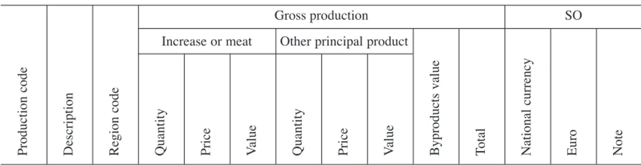
Table 2.2.a - so Calculation model for livestock productions

The first three columns of the calculation model (Table 2.2.a) identify a given production activity through a production code and a description, as well as a regional code, according to which a certain SO can be univocally attributed to a given production carried out in a certain region.

The gross production columns contain the basic data regarding amount, price and value of the meat and of the other principal product, the value of the byproducts and, finally, the total.

The three final columns contain the SO value in the national currency (for countries out-side the euro area) and in euro (the conversion rate is provided directly by the European Commis-sion to the concerned Member States), as well as notes and/or comments, if necessary.

To calculate “SO 2004” for Italy, the aforementioned model was modified by adding more columns in order to adapt it to the available data sources. Some columns were added to adapt the description of the livestock category used in ISTAT4_{statistics (the principal source we used) to}

the description given by EUROSTAT, for which the calculation of the SO is required. In fact, it should be pointed out that in some cases the breakdown of the various types of livestock into dif-ferent categories as proposed by ISTAT corresponds exactly to the production activities for which the calculation is required. However, in other cases it is necessary to group together a number of ISTAT categories or, vice versa, to split one category into several categories to obtain a grouping

P ro d u ct io n c o d e D es cr ip ti o n R eg io n c o d e Q u an ti ty P ri ce V al u e Q u an ti ty P ri ce V al u e B y p ro d u ct s v al u e T o ta l N at io n al c u rr en cy E u ro N o te Increase or meat Gross production SO

Other principal product

of data that is consistent with EUROSTAT approach. To this end, we used an adaptation coeffi-cient to convert the numerical figure, referring to live weight per head of a given livestock cate-gory as described by ISTAT statistics, into a new numerical figure referring to live weight per head of a given livestock category as described by EUROSTAT (Table 2.2.b).

Table 2.2.b – adaptation of data (source isTaT) to the eurosTaT description

Moving on to gross production, the calculation model was expanded to include other basic information needed to determine the value of the meat, i.e. the weight produced by the animal per cycle, the number of cycles in a period of 12 months and, finally, the weight produced in one year (Table 2.2.c).

Table 2.2.c – Calculation of livestock weight increase

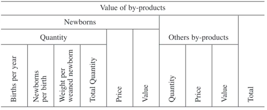
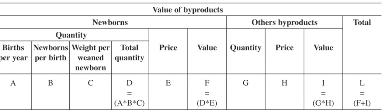
Another part of the model that was expanded was the calculation of byproducts, differen-tiated into newborns and other byproducts. In particular, columns were added to determine the number of newborns and they contain information about the number of births per year, the num-ber of newborns at each birth and the weight of the newborn at weaning (Table 2.2.d).

Table 2.2.d – Calculation of the value of by- products

C o d e D es cr ip ti o n D es cr ip ti o n L iv e w ei g h t p er h ea d A d ap ta ti o n C o d e D es cr ip ti o n L iv e w ei g h t p er h ea d

Regions Livestock category

Istat Eurostat W ei g h t p er c y cl e C y cl es p er y ea r W ei g h t pe r y ea r P ri ce V al u e Meat Live weight produced in

the category B ir th s p er y ea r N ew b o rn s p er b ir th W ei g h t p er w ea n ed n ew b o rn T o ta l Q u an ti ty P ri ce V al u e Q u an ti ty P ri ce V al u e T o ta l Newborns

Quantity Others by-products

2.3

information sources

As clearly demonstrated in the previous paragraph, determining the SO values of the live-stock productions assumes the availability of all kinds of basic data to be reprocessed according to the survey needs for each situation encountered in the course of the analysis and calculation work. Sources of information were selected, as can be expected, on the basis of their official char-acter and reliability, but also analysing their efficacy a priori in relation to the calculation method-ology intended to be used.

ISTAT statistics on livestock were the principal source used, and in particular:

- the annual data published by ISTAT on the number of heads of cattle and buffalo, sheep, goats, equines and swine as of 1 December for the years 2003, 2004 and 2005; these fig-ures provide information on the number of heads in a given region on a precise date, divided into various categories according to the type of livestock population;

- the annual ISTAT survey results for the years 2003, 2004 and 2005 of slaughtered live-stock of the following species: bovine, buffalo, swine, sheep, equine and poultry; this data provide information on the number and weight (live weight and dead weight) of the ani-mals slaughtered annually in the various regions, in some cases divided into categories; - the official statistics published by Associazione Italiana Allevatori (AIA) on the

produc-tion of milk from cows, buffalos, sheep and goats in the years 2003 - 2005; the data gath-ered on the production of milk contains information by region, province, breed and refers only to livestock farms controlled by AIA (note, however, that the trend of the number of participants in functional controls by Italian breeders is continuously rising, one reason being the higher level of professionalism they have achieved);

- the economic data of 2003, 2004 and 2005 published by Unione Nazionale dell’Avi-coltura (UNA) regarding the trends of the Italian poultry market; these data were used to obtain information about the poultry sector and conduct further analyses and comparisons between the various available sources;

- the data published by Osservatorio Nazionale della Produzione e del Mercato del miele (National Observatory of Honey Production and Market) regarding the number of beehives per region and the average regional production in the three-year period being studied; - ISTAT statistics on agricultural productions at basic prices, as shown in the Italian

Agricul-ture Yearbook of INEA, in particular for information on the quantities (especially referred to the milk) and the prices of agricultural productions during the three-year period being studied here;

- FADN information regarding livestock farms was used as a term of comparison for the above statistics and for the estimation of certain specific costs needed to calculate the SGM.

2.4

demographic models of livestock populations

As shown before, the sources of available statistics do not divide domestic livestock according to the production aptitude of the animals or, even less, according to the type of live-stock farm. On the contrary, the productions obtained from livelive-stock farms (and the relative spe-cific costs in the case of calculating the SGM) are a function of these two variables, among oth-ers. Therefore the correct “standardization” of livestock productions, requires an instrument that

considers the productions themselves according to the incidence of the various types of livestock farms on which the productions are carried out. The instrument in question is the demographic model of the bred species and its essential characteristic, for our purposes, is the distribution of the entire population of the species being studied by geographic area, age category (and/or weight and/or sex), purpose of the production (slaughter or breeding) and origin (open or closed-cycle). The methods for applying the demographic models will be explained briefly but for the moment we would like to illustrate how such models were created.

Table 2.4.a shows the demographic model of the Italian bovine and buffalo population. The data reported in it were obtained by first calculating the average three-year size of the population being examined, starting with the annual estimates of heads of livestock by ISTAT. Then, assum-ing the average regional quantity as equal to 100, we calculated the percentages of the totals of each age and sex category into which the population was divided. The percentages pertaining to the “subcategories” of each category, however, were calculated by relating to 100 the total of the item to which the “subcategories” refers. All of this excluded the number of heads of livestock destined to slaughter and coming from open-cycle farms which, on the contrary, were calculated by the difference between the percentage of livestock destined to slaughter and the percentage of suckler cows (other cows); in cases where this difference was negative, it was set at zero. The assumption underlying this estimation is that on this type of livestock farm “transit” all animals exceeding the production capacity of meat-growing farms (a number which in theory coincides with the sum of animals produced on dairy cow farms, net of imported animals and animals kept by the farm itself for internal livestock replacement). Though this assumption may initially appear exaggerated, the following considerations need to be developed:

- the percentage of animals destined for slaughter and originating from open-cycle farms is a figure needed to calculate the SO of livestock productions and therefore, having no structured information of this kind, we are compelled to estimate the figure;

- on dairy cow farms, the production of meat exceeding the amount produced from ani-mals that have reached the end of their career can be considered as a “separate manage-ment” from that of animals bred to produce milk. Therefore animals bred to produce meat on a dairy farm can simply be compared to animals from open-cycle farms.

In light of these considerations, the simplification reached by using the above-mentioned assumption can be considered entirely acceptable. The last item of information to be provided for the demographic model regards buffalo. For the purpose of calculating the SO, buffalo shall be compared to cattle. ISTAT surveys the animals in question by dividing them into two categories only: cow buffalo and other buffalo. As a result, to meet Community provisions, we should divide the other buffalo category into the same categories established for cattle. Such division was car-ried out by applying to the buffalo population the same percentage composition as that of the cat-tle population.

Table 2.4.b presents the demographic model of the domestic swine population. Data are taken from the same sources and were obtained through the same methodology already described for the demographic model of cattle. The only exception lies in the fact that, in this case, the pro-duction capacity of the closed-cycle livestock farms was not estimated according to the number of sows but that of piglets. The rationale that led to the adoption of a different method for approaching this problem was essentially as follows:

- apart from local practices which do not influence Italian food custom (e.g. the case of the Sardinian porceddu), the slaughtering of pigs is carried out according to the weight cate-gory >50 kg. The need to estimate the percentage of animals from open-cycle farms is therefore limited to this category;

- given the delicate constitution of piglets, the custom of early weaning is negligible nowa-days. We can therefore realistically state that the sale/purchase of swine does not start until they have entered the category of store pigs (just weaned, and weighing 20-25 kg); - unlike cattle, for which it is easy to hypothesize the same annual ratio for cows and

calves, the reproduction characteristics of pigs (along with the local custom of slaughter-ing piglets) are not such that they would allow the immediate ascertainment of the exist-ing annual ratio between sows and piglets. The estimation of the production capacity of closed-cycle farms starting with the number of sows would have required the need for an additional estimation to determine the number of piglets produced by these sows. Having said this, the number of pigs destined for slaughter and bred in open-cycle live-stock farms was estimated by the simple difference between the overall number of the category being examined (fattening animals) and the number of piglets5_{. It should be pointed out that the}

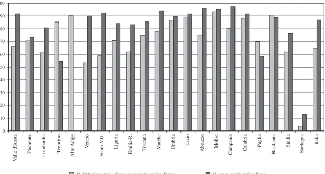
estimation criterion adopted and the results obtained are corroborated, though indirectly, in the existing ratio between piglets and sows and in the incidence of open-cycle pig farms on the total number of Italian pig farms. The piglet/sow ratio evidenced in the demographic model and calcu-lated on the basis of the same data reported in it shows, though within the confines of an accept-able regional variability, a substantial standardization of the number of animal categories being compared. The percentage incidence of open-cycle pig farms on the total number of Italian pig farms also, though referring to a different phenomenon from the one being studied here (number of farms instead of number of animals), though originating from a different source of data (census instead of short-term statistics) and though referring to a different period of time (2000 instead of the average of 2003-2005), correlates quite well with the results of the estimation made, i.e. with the percentage incidence of fattening pigs from open-cycle farms on the total number of fattening pigs. The correlation being examined is shown on chart 2.4.c.

T a b le 2 .4 .a d em o g ra p h ic m o d el o f th e it a li a n b o v in e a n d b u ff a lo p o p u la ti o n (P er ce n ta g es o f re g io n a l to ta l o r ca te g or y to w h ic h t h e "s u b ca te g o ri es " re fe rs , u n le ss o th er w is e in d ic a te d ) B o v in es u n d er o n e y ea r o ld 1 7 ,6 3 1 ,3 3 4 ,1 2 0 ,2 1 9 ,1 3 9 ,9 2 4 ,4 2 7 ,8 2 0 ,5 3 1 ,7 3 4 ,5 3 3 ,6 2 3 ,1 3 1 ,0 3 2 ,0 2 8 ,6 3 1 ,4 2 4 ,6 2 5 ,4 2 9 ,9 3 0 ,3 3 1 ,0 - to b e sl au g h te re d 4 ,7 1 4 ,2 3 0 ,6 7 ,7 4 ,7 2 8 ,8 7 ,9 1 3 ,0 7 ,7 2 4 ,9 2 0 ,0 2 5 ,4 1 5 ,7 1 7 ,5 1 7 ,1 1 3 ,6 2 6 ,1 1 4 ,0 2 0 ,0 1 7 ,2 3 0 ,0 2 2 ,8 - fr o m “ o p en ” fa rm s 3 ,7 2 ,7 2 9 ,5 7 ,1 3 ,8 2 8 ,2 6 ,5 0 ,0 5 ,1 1 2 ,3 0 ,5 9 ,2 4 ,3 5 ,6 8 ,5 2 ,5 7 ,0 8 ,5 3 ,5 0 ,0 2 ,5 1 5 ,6 - o th er s 9 5 ,3 8 5 ,8 6 9 ,4 9 2 ,3 9 5 ,3 7 1 ,2 9 2 ,1 8 7 ,0 9 2 ,3 7 5 ,1 8 0 ,0 7 4 ,6 8 4 ,3 8 2 ,5 8 2 ,9 8 6 ,4 7 3 ,9 8 6 ,0 8 0 ,0 8 2 ,8 7 0 ,0 7 7 ,2 - m al es 1 9 ,6 4 6 ,8 3 0 ,1 3 1 ,3 1 3 ,6 4 7 ,3 3 1 ,1 3 9 ,0 2 4 ,8 3 7 ,5 4 7 ,5 4 2 ,5 3 3 ,5 4 5 ,3 4 5 ,3 4 6 ,0 4 4 ,8 3 7 ,0 3 9 ,7 4 5 ,4 3 5 ,6 3 8 ,1 - fe m al es 7 5 ,7 3 9 ,0 3 9 ,3 6 1 ,0 8 1 ,7 2 3 ,9 6 1 ,0 4 8 ,0 6 7 ,5 3 7 ,6 3 2 ,5 3 2 ,0 5 0 ,7 3 7 ,2 3 7 ,7 4 0 ,4 2 9 ,2 4 9 ,0 4 0 ,2 3 7 ,4 3 4 ,4 3 9 ,1 B ov in es > 1 b ut < 2 y ea rs o ld 1 8 ,7 2 6 ,8 2 2 ,3 1 9 ,8 1 8 ,0 3 4 ,9 2 4 ,3 1 7 ,0 2 3 ,6 2 2 ,6 2 2 ,6 2 1 ,2 1 8 ,7 1 9 ,4 1 7 ,6 1 9 ,1 1 8 ,7 1 8 ,0 1 6 ,2 1 6 ,3 1 3 ,9 2 3 ,6 - m al es 8 ,5 5 5 ,1 3 3 ,6 2 1 ,5 5 ,0 6 9 ,4 3 5 ,3 3 6 ,2 3 1 ,9 5 2 ,6 6 3 ,0 5 8 ,6 3 0 ,4 5 3 ,4 5 0 ,4 5 0 ,2 6 2 ,3 2 8 ,2 3 8 ,4 4 2 ,3 3 3 ,3 4 6 ,5 - fe m al es 9 1 ,5 4 4 ,9 6 6 ,4 7 8 ,5 9 5 ,0 3 0 ,6 6 4 ,7 6 3 ,8 6 8 ,1 4 7 ,4 3 7 ,0 4 1 ,4 6 9 ,6 4 6 ,6 4 9 ,6 4 9 ,8 3 7 ,7 7 1 ,8 6 1 ,6 5 7 ,7 6 6 ,7 5 3 ,5 - to b e sl au g h te re d 1 ,1 1 2 ,5 8 ,9 5 ,5 2 ,2 1 0 ,7 7 ,9 1 9 ,8 7 ,3 2 0 ,1 1 2 ,6 11 ,7 9 ,3 8 ,5 1 3 ,8 1 5 ,0 1 0 ,5 5 ,8 7 ,9 11 ,2 8 ,4 1 0 ,0 - fr o m “ o p en ” fa rm s 0 ,1 1 ,0 7 ,8 4 ,9 1 ,2 1 0 ,1 6 ,5 0 ,0 4 ,8 7 ,5 0 ,0 0 ,0 0 ,0 0 ,0 5 ,3 3 ,9 0 ,0 0 ,4 0 ,0 0 ,0 0 ,0 2 ,8 - fo r li v es to ck f ar m 9 0 ,4 3 2 ,4 5 7 ,5 7 2 ,9 9 2 ,8 1 9 ,9 5 6 ,7 4 3 ,9 6 0 ,7 2 7 ,3 2 4 ,3 2 9 ,7 6 0 ,3 3 8 ,1 3 5 ,7 3 4 ,8 2 7 ,2 6 6 ,0 5 3 ,6 4 6 ,5 5 8 ,3 4 3 ,5 B o v in es 2 y ea rs o ld a n d o v er 1 3 ,0 9 ,1 8 ,4 6 ,7 1 0 ,1 3 ,7 7 ,2 1 4 ,5 9 ,2 1 7 ,9 11 ,9 1 3 ,3 1 3 ,0 11 ,4 6 ,3 8 ,5 1 4 ,4 9 ,3 1 2 ,2 1 2 ,6 1 5 ,6 9 ,1 - m al es 6 ,9 1 3 ,6 8 ,6 3 ,1 6 ,3 1 0 ,7 6 ,4 1 4 ,4 9 ,0 11 ,2 1 4 ,9 1 4 ,3 1 3 ,4 1 0 ,8 1 0 ,0 1 6 ,3 2 0 ,1 1 7 ,3 1 8 ,0 1 7 ,8 2 2 ,5 1 2 ,6 - fe m al es 9 3 ,1 8 6 ,4 9 1 ,4 9 6 ,9 9 3 ,7 8 9 ,3 9 3 ,6 8 5 ,6 9 1 ,0 8 8 ,8 8 5 ,1 8 5 ,7 8 6 ,6 8 9 ,2 9 0 ,0 8 3 ,7 7 9 ,9 8 2 ,7 8 2 ,0 8 2 ,2 7 7 ,5 8 7 ,4 - t o b e sl au g h te re d 0 ,9 8 ,0 3 ,7 3 ,8 4 ,6 1 2 ,6 1 2 ,3 7 ,5 5 ,3 7 ,3 6 ,0 6 ,8 8 ,1 9 ,3 1 3 ,6 1 2 ,6 8 ,4 6 ,9 9 ,1 6 ,5 6 ,1 6 ,7 - fr o m “ o p en ” fa rm s 0 ,0 0 ,0 2 ,6 3 ,1 3 ,6 11 ,9 1 0 ,9 0 ,0 2 ,8 0 ,0 0 ,0 0 ,0 0 ,0 0 ,0 5 ,0 1 ,5 0 ,0 1 ,4 0 ,0 0 ,0 0 ,0 0 ,0 - fo r li v es to ck f ar m 9 2 ,2 7 8 ,3 8 7 ,7 9 3 ,2 8 9 ,1 7 6 ,8 8 1 ,2 7 8 ,1 8 5 ,7 8 1 ,5 7 9 ,0 7 8 ,9 7 8 ,5 7 9 ,8 7 6 ,4 7 1 ,1 7 1 ,5 7 5 ,9 7 2 ,9 7 5 ,8 7 1 ,4 8 0 ,7 D ai ry c o w s 4 9 ,8 2 1 ,3 3 4 ,1 5 2 ,7 5 1 ,8 2 0 ,9 4 2 ,7 1 9 ,6 4 4 ,2 1 5 ,2 11 ,5 1 5 ,6 3 3 ,8 2 6 ,2 3 5 ,6 3 2 ,7 1 6 ,4 4 2 ,7 2 9 ,6 1 5 ,5 1 2 ,6 2 9 ,2 B u ff al o / D ai ry c o w s % 0 ,0 0 ,2 0 ,6 2 ,7 0 ,0 0 ,8 0 ,9 0 ,2 0 ,2 2 ,1 4 ,1 1 ,5 3 2 ,7 0 ,2 2 ,5 1 5 7 ,2 0 ,3 5 ,4 1 ,5 1 ,0 2 ,9 8 ,4 O th er c o w s 1 ,0 11 ,5 1 ,1 0 ,7 1 ,0 0 ,6 1 ,4 2 1 ,1 2 ,6 1 2 ,6 1 9 ,5 1 6 ,3 11 ,4 11 ,9 8 ,5 11 ,1 1 9 ,1 5 ,5 1 6 ,5 2 5 ,7 2 7 ,5 7 ,2 T o ta l b o v in es 1 ,0 0 0 h ea d s 4 1 8 3 8 1 .6 8 5 5 0 1 5 0 9 8 0 1 0 4 1 9 6 2 7 11 0 7 9 6 5 2 5 0 8 7 5 9 2 1 9 11 4 1 6 3 8 2 3 2 0 2 6 5 6 .3 0 5 T o ta l b u ff al o " 0 1 5 1 0 2 1 0 1 1 1 0 3 9 0 1 1 5 1 0 5 0 1 1 2 1 0 T o ta l b o v in es a n d b u ff al o " 4 1 8 3 8 1 .6 9 0 5 1 1 5 0 9 8 2 1 0 4 1 9 6 2 8 11 1 8 0 6 5 2 9 0 8 7 5 9 3 7 0 11 4 1 6 8 8 3 3 2 0 2 6 6 6 .5 1 5 S o u rc e: o u r p ro ce ss in g o f d a ta f ro m I S TA T val le d’a ost a pie mon te lom bar dia Tre nti no alt o a dig e ven eto fri uli -v .g . lig uri a em ili a r om ag na Tos can a Mar ch e um bri a laz io ab ru zzo Mol ise Cam pan ia Cal ab ria pu gli a bas ili cat a sic ili a sar deg na ita ly

T a b le 2 .4 .b d em o g ra p h ic m o d el o f th e it a li a n s w in e p o p u la ti o n (P er ce n ta g es o f re g io n a l to ta l o r th e ca te g o ry t o w h ic h t h e "s u b ca te g o ri es " re fe rs , u n le ss i n d ic a te d o th er w is e) w ei gh in g 50 k g or m or e s w in e fa rm s f at te n in g a n im a ls b re ed er s (l ig h t a n d h ea vy s w in e) s ow s r eg io n s < 2 0 k g fr om 2 0-50 T o ta l of w h ic h b o ar s T ot a l of w h ic h T o ta l r at io T o ta l of w h ic h (p ig le ts ) k g (y ou n g fr om “ o p en ” co v er ed (1 .0 00 h ea d s) p ig le ts / op en -c yc le p ig s) fa rm s so w s (n u m b er ) (% ) V al le d ’A o st a 1 7 ,9 2 1 ,7 5 2 ,8 6 6 ,0 0 ,1 7 ,5 8 3 ,0 0 ,7 2 ,9 3 5 9 1 ,4 P ie m o n te 1 5 ,8 2 2 ,4 5 4 ,4 7 0 ,9 0 ,1 7 ,3 8 3 ,3 9 5 4 ,1 2 ,6 1 .2 4 9 7 2 ,9 L o m b ar d ia 1 9 ,9 2 1 ,0 5 1 ,2 6 1 ,1 0 ,1 7 ,7 8 2 ,6 3 .9 6 2 ,1 3 ,1 3 .5 2 1 8 0 ,6 T re n ti n o 1 0 ,4 1 7 ,4 6 9 ,6 8 5 ,1 0 ,1 2 ,6 9 1 ,5 9 ,0 4 ,3 3 5 2 5 4 ,3 A lt o A d ig e 7 ,8 8 ,6 7 9 ,0 9 0 ,1 0 ,4 4 ,1 7 0 ,7 1 6 ,9 2 ,7 V en et o 2 2 ,2 2 1 ,2 4 7 ,1 5 2 ,9 0 ,1 9 ,4 8 4 ,5 7 1 9 ,3 2 ,8 5 .5 8 3 8 9 ,8 F ri u li -V .G . 2 0 ,7 1 9 ,7 5 0 ,2 5 8 ,8 0 ,1 9 ,3 7 3 ,4 2 1 2 ,8 3 ,0 1 .9 6 9 9 2 ,1 L ig u ri a 1 6 ,3 1 2 ,7 5 5 ,2 7 0 ,5 0 ,5 1 5 ,3 2 7, 3 2 ,9 3 ,9 1 0 0 8 4 ,0 E m il ia -R o m ag n a 1 9 ,8 2 0 ,9 5 1 ,7 6 1 ,8 0 ,1 7 ,5 8 1 ,4 1 .5 9 5 ,3 3 ,3 2 .5 9 0 8 3 ,1 T o sc an a 1 4 ,8 2 0 ,6 5 8 ,1 7 4 ,6 0 ,2 6 ,3 8 8 ,4 1 8 7 ,7 2 ,6 2 .9 0 3 8 5 ,2 M ar ch e 1 3 ,4 1 9 ,7 6 0 ,7 7 7 ,9 0 ,1 6 ,1 8 8 ,9 1 6 3 ,7 2 ,5 9 .1 1 6 9 3 ,7 U m b ri a 9 ,1 1 9 ,1 6 7 ,5 8 6 ,5 0 ,1 4 ,2 8 5 ,0 2 5 4 ,9 2 ,6 3 .7 0 3 8 9 ,5 L az io 8 ,6 9 ,9 7 7 ,7 8 8 ,9 0 ,3 3 ,5 8 0, 7 9 1 ,8 3 ,0 7 .4 2 9 9 1 ,3 A b ru zz o 1 5 ,7 1 5 ,3 6 2 ,4 7 4 ,8 0 ,2 6 ,4 8 2 ,2 11 3 ,7 3 ,0 9 .4 8 5 9 5 ,7 M o li se 5 ,5 1 2 ,3 7 9 ,1 9 3 ,0 0 ,2 2 ,9 8 4 ,4 5 1 ,6 2 ,2 4 .4 6 8 9 5 ,2 C am p an ia 1 3 ,2 1 2 ,4 6 5 ,9 8 0 ,0 0 ,2 8 ,3 8 8 ,6 1 4 5 ,0 1 ,8 1 8 .3 5 7 9 7 ,3 C al ab ri a 8 ,9 9 ,9 7 4 ,5 8 8 ,1 0 ,4 6 ,3 7 5, 1 1 2 0 ,8 1 ,9 9 .7 7 5 9 1 ,3 P u g li a 1 6 ,6 2 0 ,7 5 4 ,5 6 9 ,6 0 ,7 7 ,4 8 9 ,1 2 5 ,9 2 ,5 2 45 5 8 ,4 B as il ic at a 7 ,0 1 5 ,6 7 3 ,4 9 0 ,4 0 ,2 3 ,8 8 5 ,8 7 3 ,0 2 ,2 7 .5 1 8 8 8 ,6 S ic il ia 1 7 ,9 2 3 ,8 4 6 ,7 6 1 ,7 0 ,9 1 0 ,7 7 6, 8 4 6 ,0 2 ,2 6 1 4 7 6 ,2 S ar d eg n a 2 6 ,0 1 3 ,6 2 6 ,9 3 ,5 3 ,5 3 0 ,0 8 4 ,8 2 2 4 ,6 1 ,0 6 .0 0 4 1 3 ,0 It al y 1 8 ,6 2 0 ,3 5 2 ,8 6 4 ,7 0 ,2 8 ,1 8 2, 7 8 .9 7 1 ,8 2 ,8 9 5 .0 1 6 8 6 ,6 S o u rc e: o u r p ro ce ss in g o f d a ta f ro m I S TA T

graph 2.4.c - Correlation between open cycle swine farms and fattening swine from open cycle swine farms

Lastly, Table 2.4.d shows the demographic models of the equidae and sheep/goat popula-tions. As you can see, the information given is extremely concise and coincides with the percent-age composition of the herds of animals being studied, estimated with data found in the literature. Though concise, this information is sufficient for the previously explained objectives because, at least in Italy, the breeding of these species on open-cycle farms is lacking in statistical signifi-cance, as well as the potential variability of the composition of the different herds that can be found among the various regions.

Table 2.4.d - demographic model of the equidae and ovicaprid population

species Category % of the population

Equidae Broodmares 50

Stallions 2

Young animals 48

Ovines Ewes 60

Rams 5

“Agnelloni” lambs and wethers 15

Lambs 20

Caprines Goats breeders 60

Billys 5

Young goat/billy and wethers 15

Kid goats 20

Source: our processing of data from literature

Contrary to the above statements about equidae and sheep/goat farms, for rabbit and poul-try breeding the economic weight of the closed-cycle farms (rural farms) on the total of respective livestock farms is insignificant. Consequently, as regards the last-mentioned productions, the development of a demographic model has no meaning and was therefore ignored.

0 10 20 30 40 50 60 70 80 90 100

% fattening swine from open cycle swine farms % open cycle swine farm

Pi em on te Lo m ba rd ia Va lle d 'A os ta Tr en tin o Al to A di ge Ve ne to Fr iu li-V. G. Li gu ria Em ili a-R. To sc an a M ar ch e Um br ia La zio Ab ru zz o M ol ise Ca m pa ni a Ca lab ria Pu gl ia Ba sil ica ta Si cil ia Ita lia Sa rd eg na

2.5

Calculating gross production

2.5.1 The value of the meat: quantity and price

Our goal is to estimate the value of the meat produced by an animal6_{in one year and in the}

category to which it pertains, if a division by categories is available for the species involved. The estimation in question can be carried out by these two alternative approaches: 1) direct approach (estimation of the value of the live animal);

2) indirect approach (estimation of the value of the animal through the amount of meat it produces).

The direct approach entails the following disadvantages:

- the value of the live animal coincides with the value of the meat produced by it only for animals at the end of their production cycle. The value of the animals who are not at the end of this stage is configured more like the purchase price of a production factor and not as the sale price of a product;

- the variable “value of the live animal” is expression of a market often characterized by little transparency. Therefore, it does not necessarily coincide with the value resulting from the product between the amount of meat produced by the animal (weight of the ani-mal) and the sale price of the same. The estimation of the value in question through that of the live animal, therefore requires forgoing the use of the aforementioned information; - the failure to use the amount of meat produced by an animal leads to significant difficul-ty in calculating the costs of feeding the animal; however it should be estimated if we intend to calculate the SGM of the livestock productions. In other words, in the absence of information on the amount of meat produced by an animal, the estimation on the food consumption would necessarily produce values that are excessively standardized. On the other hand, the indirect approach, i.e. estimation of the value of the animal through the quantity of the meat it produces is relatively simple because we know its “average live weight per head” (ISTAT data –Slaughter Statistics). The only disadvantage encountered in this case, which is easily surmountable, is that the information is provided for categories that do not always univocally coincide with those contemplated by the Community typology.

In consideration of the advantages and disadvantages of each approach, it was decided to use the indirect approach. The amount of meat produced by an animal in one year and in one cat-egory was therefore calculated according to the following methodology:

- a calculation was made of the three-year average of the “average live weight per head” for each animal category contemplated by ISTAT and useful for the purposes of calculat-ing the SGM;

- each of the above categories was combined with the respective animal category contem-plated by the Community typology;

- in case of non-univocal correspondence among ISTAT categories and Community typolo-gy categories, we calculated an “adaptation coefficient” which will be discussed shortly7_;

- the average live weight per head of the animal in the various typological categories was therefore estimated by multiplying the average live weight per head for animals belong-ing to ISTAT categories by the previously mentioned adaptation coefficient.

6 _{Produced by 100 heads in the case of poultry.}

The average live weight per head clearly corresponds to the amount of meat produced by the animal in an entire production cycle, in other words a production cycle not divided into cate-gories, i.e. from birth to slaughter. The amount of meat produced by the same animal in a given category in one year was therefore calculated by subtracting from the figure in question the aver-age live weight per head of the same animal in the previous category and multiplying the figure thus obtained by the number of production cycles that the animal completes in the year. To deter-mine the amount of meat produced by the animal in the first category of each animal production and in those animal productions not divided into categories, on the contrary, we subtracted from the average live weight per head of the category (or of the production), the weight of the newborn calf just weaned or, for open-cycle productions, the weight of the replacement. All of this exclud-ed the piglets whose weight was estimatexclud-ed basexclud-ed on the average weight at birth and an average daily weight increase.

Regarding the method for estimating the weight of the newborns of the other animal species and of their replacement, we will elaborate in the next paragraphs. Currently we would only like to point out that, for the purposes of this estimation and for the reasons given in the description of the demographic models, for the cattle we considered early weaning (a one-week old calf) while, for the other animal species, we considered natural weaning.

Lastly we calculated the number of production cycles carried out by the animal in the year, by figuring the ratio between the year and the number of months the animal remains in that catego-ry, also taking into account the time needed for the “sanitary break”. Table 2.5.1.a summarizes the above-mentioned methodology and evidences the values that assume the adaptation coefficients used for the “conversion” of ISTAT categories into the typological categories and the calculation factors of the number of cycles/years carried out by the animals in their respective categories8_.

For each animal category involved (with a non-univocal correspondence), the adaptation coefficient was calculated by equaling the total weight of the ISTAT category (the average live weight per head multiplied by the number of animals) to the sum of the products obtained by multiplying the standard weight of each typological category by the number of animals belonging to it and, obviously developing the equation set up in that way according to the variable involved. Evidently the sum is made up of all, and only, the typological categories belonging to the ISTAT category being considered. For instance, in the case of cattle, the three following typological cat-egories belong to the ISTAT category “Bullocks and steer”: “Male bovine animals one but less than two years old ”, “Female bovine animals one but less than two years old” and “Heifers”. The adaptation coefficient from “Bullocks and steer” to “Male bovine animals one but less than two years old”, was then obtained by means of the following equation:

(PVMx NVM) = (PB1-2 mx NB1-2 m) + (PB1-2 fx NB1-2 f) + (PGx NG)

Where:

PVM = Live weight of bullocks and steer

NVM = Number of bullocks and steer

PB1-2 m = Live weight of male bovine animals between 1 and 2 years old

NB1-2 m= Number of male bovine animals between 1 and 2 years old

PB1-2 f = Live weight of female bovine animals between 1 and 2 years old

NB1-2 f = Number of female bovine animals between 1 and 2 years old

8 _{With the exception of the adaptation coefficients and for the factors involved in calculating the number of cycles/years completed by}

T a b le 2 .5 .1 .a s o u rc es a n d m et h o d o lo g y f o r ca lc u la ti n g t h e q u a n ti ty o f m ea t p ro d u ce d b y t h e a n im a ls o n l iv es to ck f a rm s l iv es to ck c a te g o ry Q u a n ti ty o f m ea t p ro d u ce d i n t h e ca te g o ry is T a T ( o r o th er s o u rc e) e u r o s T a T ( T y p o lo g y ) p ro d u ct io n c y cl e d es cr ip ti o n d es cr ip ti o n l iv e w ei g h t / w ei g h t g eo g ra p h ic M o n th s C yc le s/ w ei g h t h ea d p er c y cl e a re a in t h e y ea r p er y ea r ca te g o ry A B C D E F G H I L M 1 H o rs es , d o n k ey s, e tc . IS T A T 1 ,0 0 J0 1 E q u id ae = B 1 * C 1 = F 1 -n ew b o rn w ei g h t It al y 1 5 0 ,8 0 = G 1 * L 1 2 C al v es " 1 ,0 0 J0 2 B o v in es u n d er 1 y ea r o ld T o ta l = B 2 * C 2 = F 2 -n ew b o rn w ei g h t " 7 1 ,7 1 = G 2 * L 2 3 B u ll o ck s an d st ee r " 1 ,0 1 J0 3 M al e b o v in es o v er 1 b u t u n d er 2 y ea rs o ld = B 3 * C 3 = F 3 -F 2 " 1 3 0 ,9 2 = G 3 * L 3 4 B u ll o ck s an d s te er " 0 ,9 0 J0 4 F em al e b o v in es o v er 1 b u t u n d er 2 y ea rs o ld = B 4 * C 4 = F 4 -F 2 " 1 3 0 ,9 2 = G 4 * L 4 5 O x en a n d b u ll s " 1 ,0 0 J0 5 M al e b o v in es 2 y ea rs o ld a n d o v er = B 5 * C 5 = F 5 -F 3 " 9 1 ,4 0 = G 5 * L 5 6 B u ll o ck s an d s te er " 1 ,1 5 J0 6 H ei fe rs 2 y ea rs o ld a n d o v er = B 6 * C 6 = F 6 -F 4 " 9 1 ,4 0 = G 6 * L 6 7 C o w s " 1 ,0 0 J0 7 D ai ry c o w s = B 7 * C 7 = F 7 -F 6 N o rt h I ta ly -4 8 0 ,2 5 = G 7 * L 7 h il l an d m o u n ta in N o rt h I ta ly p la in 4 3 0 ,2 8 C en tr e an d S o u th I ta ly 5 2 0 ,2 3 8 C o w s " 1 ,0 0 J0 8 B o v in es 2 y ea rs o ld a n d o v er O th er c o w s = B 8 * C 8 = F 8 -F 6 It al y 8 6 0 ,1 4 = G 8 * L 8 9 S h ee p a n d R am s " 0 ,9 5 J0 9 A O v in es E w es = B 9 * C 9 = F 9 -F 1 0 " 3 0 0 ,4 0 = G 9 * L 9 1 0 “A g n el lo n i” l am bs a n d w et h er s " 1 ,1 5 J0 9 B O v in es O th er s = B 1 0 x C 1 0 = F 1 0 -n ew b o rn w ei g h t " 4 2 ,6 7 = G 1 0 * L 1 0 11 G o at s an d b il ly s " 0 ,9 5 J1 0 A C ap ri n es B re ed er s = B 11 * C 11 = F 11 -F 1 2 " 3 0 0 ,4 0 = G 11 * L 11 1 2 K id a n d y o u n g g o at s " 1 ,1 5 J1 0 B C ap ri n es O th er s = B 1 2 x C 1 2 = F 1 2 -n ew b o rn w ei g h t " 4 2 ,6 7 = G 1 2 * L 1 2 1 3 J1 1 S w in e - P ig le ts < 2 0 K g es ti m at ed v al u e = F 1 3 " 3 4 ,8 0 = G 1 3 * L 1 3 1 4 F at p ig s " 1 ,2 5 J1 2 S w in e - S o w s > 5 0 K g = B 1 4 * C 1 4 = F 1 4 -F 1 5 " 3 0 0 ,4 0 = G 1 4 * L 1 4 1 5 F at p ig s " 1 ,2 0 J1 3 S w in e - O th er s = B 1 5 * C 1 5 = F 1 5 -F 1 3 " 4 2 ,7 0 = G 1 5 * L 1 5 1 6 B ro il er s " 1 ,0 0 J1 4 B ro il er s (1 0 0 h ea d s) = B 1 6 * C 1 6 = F 1 6 -n ew b o rn w ei g h t " 2 5 ,5 0 = G 1 6 * L 1 6 1 7 L ay in g h en s " 1 ,0 0 J1 5 L ay in g h en s (1 0 0 h ea d s) = B 1 7 * C 1 7 = F 1 7 -n ew b o rn w ei g h t " 1 7 0 ,7 2 = G 1 7 * L 1 7 1 8 T u rk ey s " 1 ,0 0 J1 6 A T u rk ey s (1 0 0 h ea d s) = B 1 8 * C 1 8 = F 1 8 -n ew b o rn w ei g h t " 4 2 ,9 0 = G 1 8 * L 1 8 1 9 D u ck U N A 1 ,0 0 J1 6 B D u ck ( 1 0 0 h ea d s) = B 1 9 * C 1 9 = F 1 9 -n ew b o rn w ei g h t " 2 5 ,0 0 = G 1 9 * L 1 9 2 0 G ee se a n d g u in ea h en s " 1 ,0 0 J1 6 D O th er P o u lt ry ( G u in ea h en s) 1 0 0 h ea d s = B 2 0 x C 2 0 = F 2 0 -n ew b o rn w ei g h t " 3 4 ,0 0 = G 2 0 * L 2 0 2 1 R ab b it s IS T A T 0 ,0 4 J1 7 R ab b it s - B re ed er s = B 2 1 * C 2 1 = F 2 1 -n ew b o rn w ei g h t " 3 2 0 ,3 8 = G 2 1 * L 2 1 S o u rc e: o u r p ro ce ss in g o f d a ta f ro m d if fe re n t so u rc es pro gre ssi ve liv e wei gh t / hea d (so urc e) ad ap tat ion coe ffi cie nt Cod e

PG = Live weight of heifers

NG = Number of heifers

By developing the equation in relation to PB1-2 mwe obtain:

PB1-2 m= ((PVMx NVM) – (PB1-2 fx NB1-2 f) – (PGx NG)) / NB1-2 m

By substituting the variables of the second member of the equation, the respective values deduced from the demographic model of the cattle (numbers in the various animal categories) and from the specialized literature (standard weights in the different categories) we obtain a fig-ure which, related to the average live weight per head of the ISTAT category, provides the sought-after coefficient.

Concerning the data produced by the described methodology, the only peculiarity to make clear is a slight weight loss in the breeder cow categories, continuously in cattle and occasionally in other animal species. The amount of weight decrease9_{and slower production pace, especially}

in intensive breeding, can be considered physiological.

The prices used to put a value on the production of meat are illustrated on Table 2.5.1.b and, in this case too, we are mainly dealing with information from ISTAT source10_{(Statistics on}

National Accounts).

For the purposes of the present study, the principal limitations found when using the infor-mation in question are the following:

- like the information on physical productions, these data are determined for product cate-gories not always coinciding with the typological ones;

- the data are made available only within national boundaries.

Upon the first setback we remedied the situation by “spreading” the price actually meas-ured for one ISTAT production over several typological productions or, conversely, we “grouped” the prices measured for several ISTAT productions to arrive at the price of a typological produc-tion or, lastly, by “adapting” to certain producproduc-tions the price measured for similar producproduc-tions.

Before delving into the described operations, it should be specified that they are the only actions that allow us to obtain a set of prices that can give a value to the productions divided by typological categories and the reason is simply because the categories in question do not always correspond to the commodity categories being used in any given country. In this regard we can give one example that will make it clear: if in Italy a male or female bovine is slaughtered at 18 or 26 months, it is considered a “bullock”. It is therefore obvious that it will be very difficult to suc-ceed in defining the price of the commodity category in question by knowing details about the sex or months of life before slaughtering the animal11_{. As stated before, we should also bear in}

mind that the information to be used for the purposes of this study shall have the characteristics of an average representation of the geographical reference area. Therefore it is unlikely that detailed information can be found in the specialised literature having this characteristic. Having said this, the “spread” started with the category “Bullocks” and ended with typological categories J03, J04,

9 _{On average 9 kg/year in dairy cows and 4 kg/year in suckler cows.}

10 _{The cited source does not give the prices of categories J11, J16A, J16B and J16D; for these productions we used the prices taken}

from various sources.

11 _{The variable that determines the slaughter age of bullocks is normally the breed of the animals. Animals of the dairy breeds and also}

"light meat" breeds are usually slaughtered within the second year of life because further weight increases obtained by procrastina-ting slaughter have no economic justification. Heavier beef cattle (Chianina, Marchigiana, Piemontese, etc.), on the contrary, are usually slaughtered within the first few months of the third year of life.

T a b le 2 .5 .1 .b p ro d u ce r p ri ce s o f li v es to ck p ro d u ct io n s (n a ti o n a l a v er a g es ) p ro d u ct io n s p ri ce s (€ /k g ) is T a T c a te g o ri es e u r o s T a T c a te g o ri es C o d . d es cr ip ti o n C o d . d es cr ip ti o n w ei g h ts 2 0 0 3 2 0 0 4 2 0 0 5 a v er a g e 1 E q u id ae J0 1 E q u id ae 1 ,7 4 1 ,7 8 1 ,7 6 2 B o v in es 1 0 0 ,0 2 ,0 7 2 ,0 5 2 ,1 4 3 C al v es J0 2 B o v in es u n d er 1 y ea r o ld T o ta l 1 4 ,2 3 ,0 5 3 ,0 8 3 ,1 3 3 ,0 9 4 B u ll o ck s (m al es , fe m al es , o x en a n d b u ll s) J0 3 M al e b o v in es o v er 1 b u t u n d er 2 y ea rs o ld 7 3 ,5 2 ,0 5 2 ,0 2 2 ,0 9 2 ,0 5 J0 4 F em al e bo vi ne s ov er 1 bu t un de r 2 ye ar s ol d J0 5 B o v in es 2 y ea rs o ld a n d o v er M al es J0 6 H ei fe rs 2 y ea rs o ld a n d o v er 5 C o w s J0 7 D ai ry c o w s 1 2 ,3 1 ,0 3 1 ,0 2 1 ,2 6 1 ,1 0 J0 8 O th er c o w s 6 O v ic ap ri d s 1 0 0 ,0 2 ,8 2 2 ,7 8 2 ,8 7 7 S h ee p a n d g o at s (S h ee p ) J0 9 A O v in es E w es 2 5 ,7 0 ,9 7 0 ,9 6 0 ,9 7 0 ,9 7 8 L am b s J0 9 B O v in es O th er s 3 8 ,2 4 ,0 5 3 ,9 5 4 ,0 1 3 ,4 6 9 “A g n el lo n i” l am b s 2 8 ,6 2 ,8 9 2 ,9 0 2 ,7 6 1 0 W et h er s an d R am s 1 ,4 1 ,3 9 1 ,4 8 1 ,2 6 7 S h ee p a n d g o at s (G o at s) J1 0 A C ap ri n es B re ed er s 2 ,9 0 ,9 7 0 ,9 6 0 ,9 7 0 ,9 7 11 K id g o at s an d n ew b o rn k id s J1 0 B C ap ri n es O th er s 3 ,1 4 ,8 7 4 ,7 5 4 ,8 8 4 ,6 6 1 0 W et h er s an d R am s (K id a n d y o u n g g o at s) 0 ,2 1 ,3 9 1 ,4 8 1 ,2 6 J1 1 S w in e - P ig le ts < 2 0 K g 3 ,7 8 3 ,6 7 3 ,7 2 1 2 F at p ig s J1 2 S w in e - S o w s > 5 0 K g 1 ,2 7 1 ,2 2 1 ,2 5 J1 3 S w in e - O th er s 1 3 P o u lt ry 1 0 0 ,0 1 ,4 0 1 ,4 1 1 ,2 8 1 4 C h ic k en s J1 4 B ro il er s 9 3 ,0 1 ,4 6 1 ,4 7 1 ,3 3 1 ,4 2 1 5 H en s J1 5 L ay in g h en s 7 ,0 0 ,7 1 0 ,7 1 0 ,6 3 0 ,6 8 J1 6 A T u rk ey s 1 ,2 2 1 ,0 2 1 ,0 0 1 ,0 8 J1 6 B D u ck 1 ,3 4 1 ,3 5 1 ,2 2 1 ,3 0 J1 6 D O th er P o u lt ry ( G ee se a n d g u in ea h en s) 1 ,6 4 1 ,9 7 1 ,7 9 1 ,8 0 1 6 R ab b it s J1 7 R ab b it s - B re ed er s 2 ,1 4 2 ,1 7 2 ,1 2 2 ,1 4 S o u rc e: o u r p ro ce ss in g o f d a ta f ro m I S TA T, U N A a n d o th er s o u rc es

J05 and J06; from “Cows” to categories J07 and J08, from “Sheep and goats” to categories J09A and J10A, and from “Fat pigs” to categories J12 and J13. The grouping operation was conducted to calculate the price of the J09B category starting with the category “Lambs”, “Agnelloni lambs” and “Rams and wethers”; for category J10B we started with “Baby goats and newborn kids” and “Baby and young goats”. The operation in question is simply a weighed average calculated using the weights shown on the table above, which were also taken from ISTAT statistics. Lastly the “adaptation” was used only to define the price of the “Baby and young goats”, a category not sur-veyed by ISTAT but necessary for calculating the price of typological category J10B. The price used is that of “Rams and wethers”.

The drawback of prices availability only on the domestic market was solved by using the following methodology:

- we calculated the three-year average of the amount and values of the agricultural produc-tions reported on Table A4 of the Italian Agriculture Yearbook of INEA12_{, per region and}

for all of Italy;

- from the ratio between these two variables, we calculated the average unit value13_{of each}

production in each region and, again, for all of Italy;

- we estimated the average three-year premium per head of livestock14 _{which was then}

related to the live weight per head15_{of the animal itself. By doing this we calculated the}

premium per kg of live weight per animal;

- from the difference between the average unit value and the premium for kg of live weight we calculated the “estimated prices” of the productions being surveyed;

- from the ratio between the estimated prices of the productions in a given region and the estimated prices of the same productions nationwide, we calculated the average percent-age variations of the estimated prices which were compared to the averpercent-age percentpercent-age variations of the actual prices with respect to the average national figure. The results obtained are shown on Table 2.5.1.c;

- from the product of the price vector shown in the last column of Table 2.5.1.b and the matrix of the variations in the prices themselves shown on Table 2.5.1.c, we calculated the regional prices of the productions that were used in the study.

It should be pointed out that the entire aforementioned process, actually involved only bovines and, among Ovicaprids, only sheep and goats, because no premium is contemplated for the other productions.

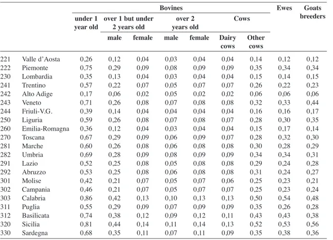
For the sake of curiosity, Table 2.5.1.d shows the premia received by the various animal categories per kilo of live weight.

12 _{In any event the source of this information is ISTAT.}

13 _{We use “average unit value” instead of “price” because the values of the productions being studied are calculated by ISTAT at}

their base prices and, therefore, they include the share of the value concerning premia related to the products (base price = produc-tion price + premia –taxes on the product).

14 _{In order to estimate the average three-year premium per head of livestock, refer to the paragraph that deals with this matter.} 15 _{Bear in mind that this refers to the live weight of the animal and not to the amount of meat produced by the animal in a year and in}

Table 2.5.1.c - average percentage variations of the average unit values of livestock productions

equidae bovines ovicaprids swine poultry rabbits

Valle d’Aosta 1,9 2,6 -0,1 8,3 23,4 -0,3 Piemonte 1,9 13,3 -4,2 -3,6 -1,1 0,3 Lombardia -1,7 -10,6 -4,0 -2,7 -9,5 0,0 Trentino -2,0 -3,4 -5,4 3,8 6,9 1,1 Alto Adige -2,0 -3,4 -5,4 3,8 6,9 1,1 Veneto -1,7 -2,9 -3,9 -1,0 -8,1 -2,2 Friuli-Venezia Giulia -1,9 1,6 -4,5 0,2 -1,4 -6,7 Liguria -2,0 -3,4 -4,2 8,5 24,9 16,9 Emilia-Romagna 6,8 -2,5 -10,0 -2,8 -1,1 -10,9 Toscana -1,8 6,1 -6,9 -1,3 9,8 8,3 Marche -1,7 16,3 -6,1 -0,8 15,3 -13,0 Umbria -0,6 6,9 -12,8 -1,6 7,5 -7,7 Lazio -1,6 14,9 -6,2 4,2 46,9 11,1 Abruzzo -1,8 9,6 -8,0 8,9 19,6 -0,7 Molise -1,3 -1,2 -8,4 2,0 11,3 1,5 Campania -1,8 2,2 -5,0 18,8 35,6 15,3 Calabria 12,4 1,5 -4,1 16,1 23,7 1,8 Puglia 5,9 9,0 -2,3 17,2 47,1 -0,4 Basilicata -1,8 -4,0 -0,3 10,0 47,2 1,0 Sicilia -1,9 7,8 17,3 8,1 -1,5 1,5 Sardegna -1,7 -4,1 1,5 28,0 14,7 9,3

Source: our processing of data from ISTAT

Table 2.5.1.d - premia per kilo of live weight (€/kg)

bovines ewes goats

under 1 over 1 but under over 2 Cows breeders

year old 2 years old years old

male female male female dairy other

cows cows 221 Valle d’Aosta 0,26 0,12 0,04 0,03 0,04 0,04 0,14 0,12 0,12 222 Piemonte 0,75 0,29 0,09 0,08 0,09 0,09 0,35 0,34 0,34 230 Lombardia 0,35 0,13 0,04 0,03 0,04 0,04 0,15 0,14 0,15 241 Trentino 0,57 0,22 0,07 0,05 0,07 0,07 0,26 0,22 0,23 242 Alto Adige 0,17 0,06 0,02 0,05 0,02 0,02 0,06 0,06 0,06 243 Veneto 0,71 0,26 0,08 0,07 0,08 0,08 0,32 0,33 0,44 244 Friuli-V.G. 0,39 0,14 0,04 0,04 0,04 0,04 0,16 0,16 0,17 250 Liguria 0,59 0,26 0,08 0,07 0,08 0,07 0,28 0,30 0,35 260 Emilia-Romagna 0,36 0,12 0,04 0,03 0,04 0,04 0,15 0,17 0,14 270 Toscana 0,67 0,29 0,09 0,06 0,09 0,07 0,28 0,32 0,30 281 Marche 0,60 0,26 0,08 0,06 0,08 0,08 0,30 0,28 0,29 282 Umbria 0,69 0,28 0,09 0,08 0,09 0,09 0,34 0,34 0,31 291 Lazio 0,52 0,25 0,08 0,05 0,08 0,08 0,29 0,24 0,28 292 Abruzzo 0,53 0,25 0,08 0,06 0,08 0,08 0,31 0,24 0,27 301 Molise 0,42 0,21 0,07 0,05 0,07 0,06 0,25 0,23 0,21 302 Campania 0,46 0,21 0,07 0,05 0,07 0,07 0,25 0,23 0,24 303 Calabria 0,86 0,42 0,13 0,10 0,13 0,13 0,50 0,54 0,48 311 Puglia 0,55 0,29 0,09 0,07 0,09 0,09 0,35 0,26 0,28 312 Basilicata 0,74 0,38 0,12 0,09 0,12 0,11 0,43 0,43 0,38 320 Sicilia 0,81 0,44 0,14 0,11 0,14 0,13 0,52 0,53 0,56 330 Sardegna 0,68 0,35 0,11 0,07 0,11 0,09 0,35 0,38 0,36

2.5.2 The value of milk, eggs and honey: quantity and price

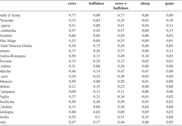
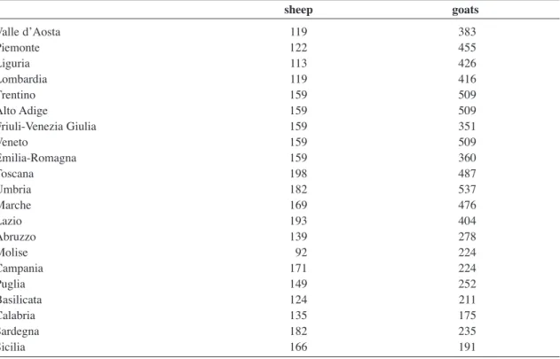
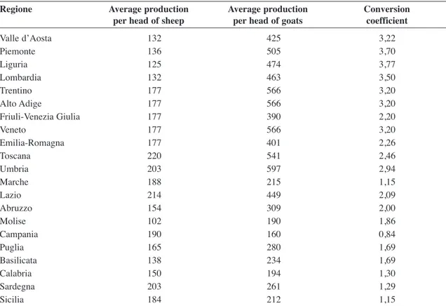
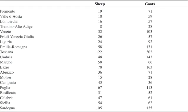
Milk, eggs and honey are the principal productions for certain categories of livestock: milk for dairy cows, sheep and goats, eggs for laying hens and honey for bees. Milk represents a sec-ondary production in the category of other cows (suckler cows) as they have calves as their prin-cipal product.

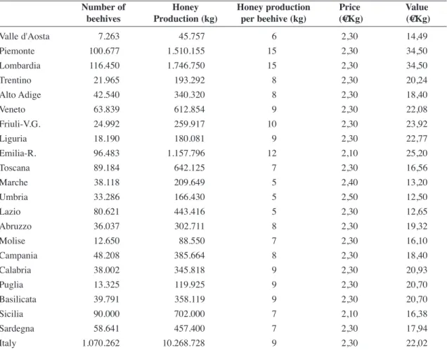
The information needed to determine the SO is naturally the quantity and the price. The amount of milk produced was calculated based on ISTAT data on agricultural produc-tions and AIA data on the production of bovine, buffalo, sheep and goat milk. The number of eggs was estimated at 300 per head per year (30,000 per 100 heads), because we chose to take into consideration only intensive poultry farms since they make up over 90% of the Italian market of poultry productions. Lastly, for the amount of honey produced per region and per beehive in one year we used the data published by the Honey Observatory.

Bovine and buffalo milk

The basic data from ISTAT source used to calculate bovine and buffalo milk produced per head on average in the three-year period in question referred to the milk of cows and buffaloes considered as a unitary figure; this information is required for the purposes of determining the SO; since buffalo productions should be considered (and calculated) as one with bovine produc-tions within the category of dairy cows. In fact, this methodological constraint overestimates the production of buffalo milk. Nonetheless, given the low relative incidence of this production on the total, the explicative significance of the model is not misinterpreted.

Two production activities require a calculation of the value of bovine and buffalo milk: J07 Dairy cows and J08 Other cows. In this last-mentioned case, though suckler cows, we thought it would have been proper to also consider the milk as a production destined to the market, though only limited to the surplus amount not needed to feed the calves.

Since available data refer to the total cow and buffalo milk production per region, we have to separate from this amount the production of milk attributed to “Other cows”. To this end, on the basis of the indications found in the literature regarding milk production of the principal breeds of beef cows, we estimated the average amount of milk produced by one suckler cow which exceeded the milk amount destined to the calf. The regional average amount of milk des-tined to the sale attributed by estimate to the suckler cow, multiplied by the average number of “Other cows” during the three-year period allows determining the amount of milk produced by the latter in each region. Subtracting this value from the total amount of milk produced by cows and buffaloes in each region, we obtain by difference the milk produced by the dairy cows. This was then divided by the average population of dairy cows in the three-year period, allowing us to obtain the milk produced by each dairy cow in each region (Table 2.5.2.a).