C L A S S E D I S C I E N Z E M AT E M AT I C H E E N AT U R A L I
Corso di Perfezionamento in N A N O S C I E N Z E
T H E R M A L T R A N S P O R T I N S TAT I C A N D D R I V E N N A N O S C A L E
Q UA N T U M S Y S T E M S
tesi di perfezionamento
Candidato
Relatori
bibek bhandari
prof. rosario fazio
dr. fabio taddei
Bibek Bhandari: Thermal transport in static and driven nanoscale quantum systems, Tesi di Perfezionamento, © Anno Accademico 2019/2020
P U B L I C AT I O N S
Bibek Bhandari, Giuliano Chiriaco, Paolo Andrea Erdman, Rosario Fazio and Fabio Taddei, Thermal drag in electronic conductors,Phys. Rev. B, 98, 035415 (2018)
Paolo Andrea Erdman, Bibek Bhandari, Rosario Fazio, Jukka Pekola and Fabio Taddei, Absorption refrigerators based on Coulomb-coupled single-electron systems,Phys. Rev. B, 98, 045433 (2018)
Paolo A Erdman, Joonas T Peltonen, Bibek Bhandari, Bivas Dutta, Herve Courtois, Rosario Fazio, Fabio Taddei, Jukka P Pekola, Nonlinear thermovoltage in a single-electron transistor,Phys. Rev. B, 99, 165405 (2019)
Olivier Maillet, Paolo A Erdman, Vasco Cavina, Bibek Bhandari, Elsa T Man-nila, Joonas T Peltonen, Andrea Mari, Fabio Taddei, Christopher Jarzynski, Vittorio Giovannetti, Jukka P Pekola, Optimal probabilistic work extraction be-yond the free energy difference with a single-electron device,Phys. Rev. Lett, 122, 150604, (2019).
Bibek Bhandari, Pablo Terren Alonso, Fabio Taddei, Liliana Arrachea, Felix Von Oppen and Rosario Fazio, Geometric properties of adiabatic quantum thermal machines,Phys. Rev. B, 102, 155407 (2020).
Michele Governale, Bibek Bhandari, Fabio Taddei, Ken-Ichiro Umura and Uli Zülicke, Finite-size effects in cylindrical topological insulators,New Journal of Physics, 22, 063042 (2020).
Bibek Bhandari, Rosario Fazio, Fabio Taddei and Liliana Arrachea, Quantum coherent adiabatic dynamics: Derivation of quantum master equations from Keldysh NEGF, in progress.
Bibek Bhandari, Paolo Andrea Erdman, Rosario Fazio, Elisabetta Paladino and Fabio Taddei, Heat Rectification in low-dimensional quantum systems, in progress.
R I N G R A Z I A M E N T I
Desidero esprimere la mia sincera gratitudine a tutti coloro che mi hanno aiutato durante il mio dottorato.
Ringrazio infinitamente il professor Rosario Fazio, e il Dr. Fabio Taddei: senza il loro supporto e la lora guida non sarei mai arrivato a questo tra-guardo.
Vorrei ringraziare tutte le persone che mi hanno dato una mano quando ne avevo bisogno: i miei amici e insegnanti sia in Italia che in Nepal, la mia famiglia e la mia fidanzata.
Infine, dedico questo lavoro a mio ‘pitaji’ e a mia ‘ammijaan’.
C O N T E N T S
1 introduction 1
2 model and formulation 5
2.1 Model . . . 5 2.1.1 System . . . 5 2.1.2 Baths . . . 6 2.1.3 Coupling . . . 7 2.2 Heat Current . . . 8 2.2.1 Static case . . . 9 2.2.2 Driven case . . . 9
3 thermodynamics and thermal machines: a brief review 13 3.1 Transport theories and thermoelectrics in nanoscale quantum systems . . . 14
3.2 Heat transfer and thermodynamics in nanoscale devices . . 16
3.3 Experiments on nanoscale quantum thermal devices . . . 19
4 thermal drag in coulomb coupled single electron systems 21 4.1 Thermal Drag in Coulomb coupled Metallic islands . . . 23
4.1.1 Sequential tunneling regime . . . 24
4.1.2 Co-tunnelling contributions . . . 30
4.1.3 Superconducting electrode . . . 31
4.2 Thermal Drag in Coulomb coupled Quantum dots . . . 34
4.2.1 Formulation . . . 35
4.2.2 Energy dependent tunneling – Charge-state-dependent transition amplitudes . . . 36
4.2.3 Energy Dependent Tunneling - Superconducting Electrode . . . 37
4.2.4 Order dependence on bias . . . 38
4.3 Summary . . . 39
5 absorption refrigerators based on coulomb coupled single-electron devices 41 5.1 Model . . . 41 5.2 Quantum dots . . . 44 5.3 Metallic islands . . . 46 5.4 Summary . . . 48 6 thermal rectification 49 6.1 Model . . . 52
6.2 Heat Current and Rectification . . . 52
6.3 Qubit: Weak coupling regime . . . 53
6.3.1 Rectifying with “similar” system-bath coupling . . . 54
6.3.2 Arbitrary baths with different spin couplings to the system . . . 55
6.3.3 Rectification enhanced by the Lamb-Shift . . . 56
6.4 Qubit: Beyond Weak Coupling Regime . . . 57
6.4.1 Master equation with co-tunneling . . . 58
6.4.2 Non-equilibrium Green’s function method . . . 59
6.4.3 Spin-boson model: Exact calculation . . . 60
6.4.4 Rectification beyond the weak-coupling regime . . . 61
6.4.5 Rectification with arbitrary s coupling . . . . 64
viii contents
6.5 Non-linear quantum circuit . . . 66
6.5.1 Results . . . 69
6.6 Coulomb coupled quantum dots . . . 71
6.7 Summary . . . 74
7 thermal transport in single electron devices: exper-iment and theory 75 7.1 Nonlinear thermovoltage in a single-electron transistor . . . 75
7.2 Setup . . . 76
7.3 Results . . . 77
7.4 Optimal probilistic work extraction beyond free energy dif-ference . . . 80
7.5 Summary . . . 85
8 geometric properties of adiabatically driven quan-tum systems 87 8.1 Model of a geometric thermal machine . . . 89
8.1.1 Heat, work, and operational modes . . . 90
8.1.2 Adiabatic forces, currents, and entropy production over a cycle . . . 91
8.2 Geometric characterization . . . 93
8.2.1 Thermal geometric tensor . . . 93
8.2.2 Thermal machines and geometry . . . 94
8.2.3 Efficiencies . . . 97
8.3 Examples . . . 98
8.3.1 Driven qubit . . . 98
8.3.2 Driven quantum dot . . . 108
8.4 Summary . . . 116
9 quantum coherent dynamics of adibatically driven systems 119 9.1 General formalism . . . 121
9.1.1 Model . . . 121
9.1.2 Dynamics of the density matrix . . . 122
9.1.3 Dynamics of the particle and energy current between system and baths . . . 125
9.1.4 Power developed by the ac forces . . . 125
9.2 Adiabatic dynamics . . . 125
9.2.1 Full adiabatic master equation . . . 127
9.3 Examples . . . 128
9.3.1 Qutrit . . . 128
9.3.2 Coupled quantum dots . . . 131
9.3.3 Thermal Rectification . . . 133
9.4 Summary . . . 135
10 conclusions 137 a appendix 1 139 a.1 Quantum master equations using Fermi Golden rule . . . . 139
a.1.1 Sequential tunneling rates . . . 139
a.1.2 Cotunneling rates . . . 140
b appendix 2 143 b.1 Keldysh-Schwinger formulation based on non-equilibrium Green’s function . . . 143
b.1.1 Static systems . . . 145
b.1.2 Driven systems . . . 145
c appendix 3 149 c.1 Kubo formulation : Linear response . . . 149
contents ix
c.1.1 Luttinger theory of thermal transport . . . 149
c.1.2 Adiabatic Response . . . 150
d appendix 4 155 d.1 Master equations for two capacitively-coupled islands . . . . 155
d.2 Charge and heat transition rates for co-tunneling . . . 156
d.2.1 Derivation . . . 157
d.3 Charge and heat current in the co-tunneling regime . . . 162
e appendix 5 163 e.1 Master Equation . . . 163
e.2 Optimal rates for cooling power and COP . . . 164
e.3 Derivation of the master equation for the system with three QDs . . . 164
e.4 Heat currents in the system with metallic islands . . . 166
f appendix 6 169 f.1 Most Generic System-Bath Coupling . . . 169
f.2 Rectification in the weak coupling regime . . . 169
f.3 Tunneling Rates . . . 170
f.4 Tunneling Rates in Specific Models . . . 171
f.4.1 Fermionic baths with linear (tunnel) couplings . . . 171
f.4.2 Bosonic baths with linear (tunnel-like) coupling . . . 171
f.4.3 Arbitrary baths with different s couplings . . . . 172
f.5 Thermal Averages . . . 172
f.6 Lamb shift . . . 173
f.7 Co-tunneling calculation . . . 174
f.8 Non equilibrium Green’s function calculation . . . 176
f.8.1 Derivation of Green’s function . . . 177
f.8.2 Calculation of Dyson equation . . . 178
f.8.3 Calculation of Currents for simple models . . . 181
f.8.4 Exact calculation . . . 182
f.9 Quantum non-linear circuit . . . 186
g appendix 7 189 g.1 Driven qubit: Calculation of currents and power for different spin couplings . . . 189
g.1.1 Coupling: ˆtL = ˆsxand ˆtR= ˆsz . . . 189
g.1.2 Coupling: ˆtL = ˆsxand ˆtR= ˆsy . . . 189
g.1.3 Symmetry properties of L`,`0 . . . 190
g.2 Driven quantum dot - calculation of the thermal geometric tensor . . . 190
h appendix 8 193 h.1 Evaluation of the mean values . . . 193
h.2 Calculation of coefficients of the frozen master equation . . 194
h.3 Adiabatic dynamics . . . 194
h.3.1 Lesser Green’s function . . . 194
h.3.2 Greater Green’s function . . . 195
h.4 Calculation of master equations for a qutrit . . . 196
h.4.1 Frozen Dynamics . . . 198
h.4.2 Adiabatic dynamics . . . 199
h.5 Calculations of energy current in the case of qutrit . . . 200
h.6 The Lindblad form . . . 200
1
I N T R O D U C T I O NQuantum transport and thermodynamics at nanoscale has been a subject of growing interest in modern research for some time. It is a widely studied field and ranges from the theoretical study of nanoscale devices using the principles of statistical and quantum mechanics to the experimental realisa-tion of those devices. In addirealisa-tion, the field of nanoscience has represented itself as a common playground for physicists, chemists, material scientists, biologists as well as engineers. The main motivation being the theoretical pro-posal and experimental realisation of devices with novel properties emerging at the nanoscale. Moreover, the interest in this field has been further bolstered by the fact that the nanoscale devices have a wide range of application, from electronic and thermal devices to quantum computers. The inevitable appli-cation of quantum mechanics at this scale gives rise to interesting physics not observed in the classical regime. For instance, quantum Hall effect, quan-tized adiabatic pumping and so on. On the other hand, transistors used in contemporary computers and other electronic devices have the size of around 20 nm. Therefore, modern devices are already at the nanoscale and further miniaturisation of these devices makes the understanding of energy dynamics in this regime essential. The fabrication and application of devices at such a small scale entails serious technical challenges: noise and heat dissipation are the most significant ones.
When the system is attached to two reservoirs, thermal transport can be mediated by maintaining a thermal or potential bias, or by driving in time the system parameters. When it comes to nanoscale devices, thermal transport becomes as significant as particle transport. This has led to the invention of devices based on thermal transport such as thermal transistors and thermal diodes. Quantum thermodynamics governs the statistics, work production, entropy and other thermodynamic quantities in the quantum regime. To summarize, the study of thermal transport and thermodynamics at nanoscale not only helps in understanding the physics at nanoscale but also presents novel direction for technological advancement along with the miniaturisation of devices. Arguably, quantum transport and quantum thermodynamics have become the leading subject of interest in nanoscience.
In this thesis, we shall study quantum transport and quantum thermody-namics in nanoscale using different techniques (quantum master equation[1,
2], non-equilibrium Green’s function[3,4], linear response theory[5,6]). We will be mainly focused on heat dynamics in the static as well as driven systems (for example quantum dots, metallic islands, resonators and qubits) attached to thermal reservoirs.
When we discuss about a modern field in science, for example thermal transport in nanoscale which has been so widely studied, there is always a problem of being too specific or too general. When we are too specific, there is a good chance we miss the forest for the details of the trees. On the other
2 introduction
hand, being too general might give us an over all comprehensive picture, but might render the discussion impractical or even inapplicable due to the lack of technical details. Although a balance between these two fronts is highly desirable, mostly it becomes inevitable to sacrifice one for the other. In order to address this issue, in the first three chapters we shall provide a general but a brief review on thermal transport and thermodynamics in nanoscale systems. In the last six chapters (from Chapter IV to Chapter IX), we will discuss about the specific properties and applications of thermal transport in static and driven nanoscale devices.
In particular, in Chapter II we will introduce different models of nanoscale devices that will be studied in the forthcoming chapters. We will also present a microscopic derivation of heat current for static as well as driven systems using Keldysh non-equilibrium Green’s function.
In Chapter III, we will give a brief review of thermodynamics and thermal machines. We will talk about both theoretical and experimental develop-ments in the field of classical as well as quantum thermodynamics, thermal transport and thermoelectrics.
In chapter IV, we will study the electronic thermal drag in two different Coulomb-coupled systems, the first one composed of two Coulomb block-aded metallic islands and the second one consisting of Coulomb coupled quantum dots. The two conductors of each system are electrically isolated and placed in the two circuits (the drive and the drag) of a four-electrode setup. The systems are biased, either by a temperature DT or a voltage V difference, on the drive circuit, while no biases are present on the drag circuit. We will use a master equation approach to determine the general properties of the dragged heat current, accounting also for co-tunneling contributions and the presence of large biases. Analytic results will be obtained in the sequential tunneling regime for small biases, finding, in particular, that the drag heat current is quadratic in DT or V and non-monotonous as a function of the inter-island coupling. Finally, by replacing one of the electrodes in the drag circuit with a superconductor or taking charge state dependent transition rates (in the case of quantum dots), we will find that heat can be extracted from the other normal electrode.
In chapter V, we will analyze a simple implementation of an absorption refrigerator, a system that requires heat and not work to achieve refrigeration, based on two Coulomb-coupled single-electron systems. We will determine the general condition to achieve cooling-by-heating. We will propose two possible experimental setups based on quantum dots or metallic islands that implement the nontrivial cooling condition. Using realistic parameters, we will show that these systems, which resemble existing experimental setups, can develop an observable cooling power.
In chapter VI, we will study thermal rectification. We will present a com-prehensive and systematic study of thermal rectification in low-dimensional quantum systems. Focusing on various prototypical systems - a qubit, a non-linear harmonic oscillator and a Coulomb coupled quantum dot system - we identify necessary conditions to observe thermal rectification and we discuss strategies to maximize it. In particular, in the qubit case we will derive general upper bounds on rectification which hold in the weak system-bath coupling regime, and we show how the Lamb shift can be exploited to enhance rectification. We then go beyond the weak coupling regime using the non-equilibrium Green’s function formalism and the Feynman-Vernon path integral approach. We will find that the strong coupling regime allows us to violate the bounds derived in the weak coupling regime, providing us
introduction 3 with clear signatures of high order coherent processes visible in the thermal rectification. In the non-linear harmonic oscillator, we will study the heat rectification using two different approximate schemes 1) mean field Hartree approximation and 2) equation of motion method that goes beyond mean field. The mean field calculations reproduces the results of the equation of motion method when the interaction is small compared to other energy scales of the system. Thermal rectification is enhanced in the large interaction limit, making equation of motion better suited to study thermal rectification in non-linear resonators. Finally, we will study non-local thermal rectification in Coulomb coupled quantum dots. For a suitable choice of parameters, we will show that a perfect non-local thermal rectification can be obtained.
In chapter VII, we will study thermal transport in two different single electron devices using master equations. In the first section, we will theoreti-cally reproduce the experimental results of thermovoltage measurements in a single-electron transistor, both in the linear and non-linear regimes. Using a model which accounts for co-tunneling, we will find excellent agreement with the experimental data with no free parameters even when the tem-perature difference is larger than the average temtem-perature (far-from-linear regime). This will allow us to confirm the sensitivity of the thermovoltage on co-tunneling and to find that in the non-linear regime the temperature of the metallic island is a crucial parameter. In the second section, using master equations we will theoretically match the experimental results for work extraction (beyond the free energy difference) from a single electron transistor at the single thermodynamic trajectory level. With a carefully designed out-of-equilibrium driving cycles featuring kicks of the control parameter, we will demonstrate work extraction up to large fractions of kBT,
despite zero free energy difference over the cycle. Our results are explained in the framework of nonequilibrium fluctuation relations. We thus shall show that irreversibility can be used as a resource for optimal work extraction even in the absence of feedback from an external operator.
In chapter VIII, we will present a general unified approach for the study of quantum thermal machines, including both heat engines and refrigerators, operating under periodic adiabatic driving and in contact with thermal reser-voirs kept at different temperatures. We will show that many observables characterizing this operating mode and the performance of the machine are of geometric nature. Heat-work conversion mechanisms and dissipation of energy can be described, respectively, by the antisymmetric and sym-metric components of a thermal geosym-metric tensor defined in the space of time-dependent parameters generalized to include the temperature bias. The antisymmetric component can be identified as a Berry curvature, while the symmetric component defines the metric of the manifold. We will show that the operation of adiabatic thermal machines, and consequently also their efficiency, are intimately related to these geometric aspects. We will illustrate these ideas by discussing two specific cases: a slowly driven qubit asymmet-rically coupled to two bosonic reservoirs kept at different temperatures, and a quantum dot driven by a rotating magnetic field and strongly coupled to electron reservoirs with different polarizations. Both examples are already amenable for an experimental verification.
In chapter IX, we will present a systematic derivation of the quantum mas-ter equation which describes the adiabatic dynamics of a driven quantum system weakly coupled to reservoirs kept at different temperatures. Starting from the microscopic Hamiltonian, we will derive such quantum master equa-tion by means of the Schwinger-Keldysh non-equilibrium Green’s funcequa-tions
4 introduction
performing a perturbation expansion in the coupling between the system and the reservoirs. We will also calculate the charge and energy fluxes, as well as the power developed by the driving forces within the same framework. We will analyze the instantaneous as well as adiabatic contributions to the diagonal and off-diagonal elements of the density matrix in two specific ex-amples, namely a qutrit attached to bosonic reservoirs and a pair of coupled quantum dot attached to fermionic reservoirs. Finally, we will also study heat rectification in adiabatically driven systems.
In Appendices A, B and C, we shall give a brief introduction of all the formulations used in the thesis to study thermal transport in nanoscale quan-tum devices: quanquan-tum master equation formulation based on Fermi golden rule will be presented in Appendix A, Keldysh-Schwinger formulation based on non-equilibrium Green’s functions will be presented in Appendix B and Kubo formulation based on Luttinger theory of thermal transport in Appendix C.
2
M O D E L A N D F O R M U L AT I O NIn this chapter, we will present different nanoscale devices that will be studied in the upcoming chapters. We will also present a microscopic derivation of heat current for static and driven systems which would be essential to study thermal transport properties of specific devices in upcoming chapters. 2.1 model
T
L
S
T
R
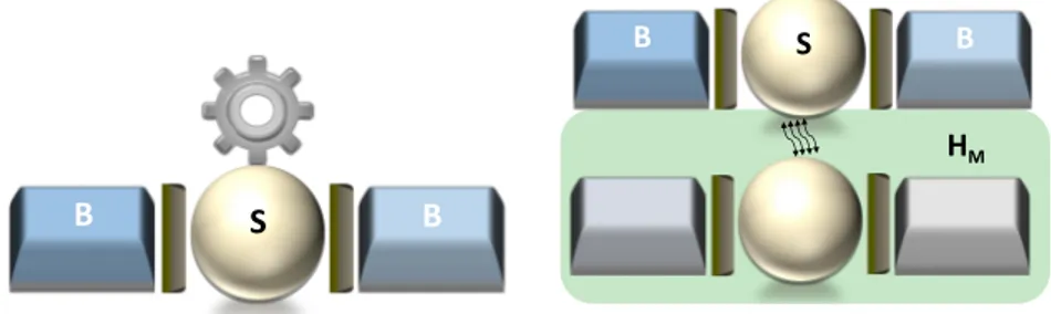
Figure 2.1: A nanoscale system S connected to baths L and R. A thermal and a potential bias has been maintained between the two baths.
As shown in Fig. (2.1), a nanoscale device is composed of three components, 1) system, 2) baths and 3) contacts. The baths represented by red and blue blocks on the two sides of the system (S) can be maintained at a thermal or potential bias. The total Hamiltonian is given by
H=HS+HB+HC, (2.1)
where HSrepresents the Hamiltonian for the system, HBrepresents the bath
Hamiltonian and HCgives the coupling between the system and the baths.
2.1.1 System
We will generally consider three different type of systems: 1) fermionic, for example quantum dots and metallic islands, 2) bosonic, for example resonators. The Hamiltonian for a quantum dot is given by:
HQD =
Â
i eia†iai+Â
i wi ⇣ a†iai+1+h.c. ⌘ +Â
i6=jUijn † inj, (2.2) 56 model and formulation
where ai(a†i)represent the fermionic annihilation (creation) operator of the
electron in the quantum dot (QD) labelled by i, Uijrepresents the inter-dot
Coulomb interaction between QDs i and j, ei is the onsite potential of
quan-tum dot i and wigives the tunneling strength between QD i and i+1. The
inter-dot Coulomb interaction will serve for studying non-local thermoelec-tric phenomena. The fermionic annihilation and creation operators satisfy the commutation relations, ai, a†i =1. The Hamiltonian for Coulomb coupled
metallic islands is given by HMD=
Â
k,i=1,2
ekia†kiaki+U
Â
k,k0nk1nk02. (2.3)
The strength of inter-metallic island Coulomb interaction is given by U, eki
represents the energy of mode k in the metallic island i and aki(a†ki)is the
fermionic annihilation (creation) operator of an electron in metallic island i. The Hamiltonian for a single mode harmonic resonator is
HR=Db†b+Ub†b†bb, (2.4)
where D gives the frequency of the resonator, the strength of non-linearity is determined by U and b(b†)represents the bosonic annihilation (creation)
operator of the resonator. The bosonic operators satisfy the commutation relation,⇥b, b†⇤=1.
Finally, the qubit Hamiltonian is
HQ= D2sz, (2.5)
where D gives the qubit gap. 2.1.2 Baths
The baths are considered to be macroscopic systems with continuous degrees of freedom. The baths have a large enough heat capacity and are at thermal equilibrium with a fixed temperature Taand chemical potential µa. Since the baths are kept at thermal equilibrium, the statistics of the baths can be defined by a thermal Gibbs state ra =e Ha/kBTa/Za, where Hais the Hamiltonian of the bath a with partition functionZa =Tr
h
e Ha/kBTai. When the baths
maintained at a thermal or potential gradient are connected to a system, thermal conduction takes the bath out of thermal equilibrium. Due to the presence of inelastic scattering, the baths quickly attain thermal equilibrium. We consider that the time scale corresponding to the attainment of thermal equilibrium is the smallest time scale. In other words, the dynamics of bath is fast enough compared to the dynamics of the system. In this scenario, the coarse grained Markov approximation will be valid, provided the system-bath coupling is weak. The Hamiltonian of the Bosonic (B) and Fermionic (F) baths are given by
HBa =
Â
k ekab†kabka, (2.6) HaF =Â
k (eka µa)c†kacka, (2.7) where bka(cka)and b†ka(c †ka)are the creation and annihilation operators for
bosons (fermions) with energy eka for bath a. These operators satisfy the
usual commutator and anti-commutator relations,⇥bka, b†k0a0
⇤
=dkk0daa0and
2.1 model 7 2.1.3 Coupling
In general, we will consider a linear system-bath coupling. The coupling acts as a medium for the exchange of energy and particle between the system and the baths. The coupling contains both system and bath degrees of freedom, so it changes when either the system or bath changes. In the case of quantum dot i attached to fermionic bath a, the coupling Hamiltonian takes the form
Ha,QD =
Â
kVkaa†icka+h.c. (2.8)
For the case of a metallic island, the coupling Hamiltonian should be modi-fied to address the continuous energy modes in the system, i.e.
Ha,MD=
Â
k,q
Vkq,aa†kicqa+h.c. (2.9)
In the case of single mode harmonic resonator attached to bosonic bath the Hamiltonian takes the form
Ha,R=
Â
k Vka ⇣ b†ka+bka ⌘ ⇣ b†+b⌘. (2.10) For the sake of simplicity, in some cases we will take only the particle conserving term in the latter contact Hamiltonian such that the coupling Hamiltonian for a single mode resonator connected to bosonic baths reduces toHa,R=
Â
k
Vkab†kab+h.c. (2.11)
Finally, the most general system-bath interaction for a qubit is given by Ha,Q=
Â
k Vk ⇣ bka⌦s++b†ka⌦s ⌘ +Baz⌦sz+Ba1⌦1, (2.12)where Baz and Ba1 are Hermitian operators acting on the space of bath a. When we shall consider arbitrary spin coupling between the qubit and the bosonic baths, we will use a modified version of coupling Hamiltonian given by Ha,Q=
Â
k VkaÂ
i=x,y,z mi,asi⌦ ⇣ bka+b†ka ⌘ , (2.13)where ma = (sin qacos fa, sin qasin fa, cos qa)is a unit vector parameterized by the angles qaand fa.
As we will see in the following chapters, the system-bath interaction can be conveniently characterized by the spectral density
Ga(e) =2p
Â
k
d(e eak)VakVa⇤k. (2.14) In the following, we will consider generic spectral densities for the two baths. In the cases of bosonic baths, we will consider Ohmic spectral densities with an exponential cut-off energy eC (unless mentioned otherwise), i.e.
Ga(e) =pKaee e/eC ⌘KaI(e), (2.15) where Ka is the dimensionless Ohmic coupling strength [7]. And for the fermionic baths, we will generally consider characterless spectral density given by
8 model and formulation 2.2 heat current
We are interested in studying the steady-state heat current flowing across the device when a temperature bias is imposed between the baths. Specifically, as depicted in Fig.2.1, we fix TL=T+DT/2 and TR=T DT/2, where T
is the average temperature. Even in the fermionic case, we will consider the case of zero chemical potential. Furthermore, since we consider steady state currents, the heat flowing out of one bath is equal to the one flowing into the other bath. In addition, in the absence of chemical potential the heat current and energy current are the same, i.e. J(h)a =Ja(E). Therefore, for simplicity we define the heat flowing out of the left lead as
Ja(h)(DT)⌘ lim
t!+•
d
dthHai (t), (2.17) whereh. . .i (t) =Tr[r(t). . .], r(t)being the density matrix representing the state of the total system at time t. Notice that the time variation of the energy associated with the coupling Hamiltonian vanishes in steady state [8]. In addition, since the energy current is conserved we have, JL(E)= JR(E)= J(E).
Starting from the formal definition of the heat current given in Eq. (2.17), we can simplify the calculation of the heat current using a standard procedure known as “bath embedding”[4], which is valid whenever the operators of the bath appear linearly in Ha,S. This approach applies to all models with linear coupling between the system and the baths. Under such hypothesis, the formally exact Meir-Wingreen-type formula [9] for the heat current can be written as [10,11,12,13,14] Ja(h)(t) =⌥2
Â
k eka|Vka|2 Z dt1Re⇥GrSS(t, t1)g<ka(t1, t) +G<SS(t, t1)gaka(t1, t)⇤, (2.18) where S is the system degree of freedom in the contact Hamiltonian Ha,S(see Subsection (2.1.3)): in the quantum dot case S ⌘ ai where ai is the
annihilation operator of the quantum dot i attached to bath a, in the case of metallic islands S⌘akiwhere aki is the annihilation operator of the metallic
island i attached to bath a, in the case of resonator with resonator bath coupling defined through Eq (2.10), S⌘b†+b where b†(b)are the creation
(annihilation) operator for the resonator attached with bath a and for the case of qubit S=Âi,ami,asiwhere mi,a associated with coupling to bath a is
defined below Eq. (2.13). The minus sign in front of the integral applies only when both the system and the baths are fermionic. The greater and lesser Green’s functions for the system are respectively defined as
G> SS(t, t0) = i D S(t)S†(t0)E G< SS(t, t0) =±i D S†(t0)S(t)E, (2.19)
with the retarded Green’s function Gr
SS(t, t0) =q(t t0)[GSS>(t, t0) GSS<(t, t0)].
The greater and lesser Green’s function for the bath a can be similarly defined as
g>
ka(t, t0) = ihdka(t)d†ka(t0)i
g<
ka(t, t0) =±ihd†ka(t0)dka(t)i, (2.20)
respectively with the retarded Green’s function gr
ka(t, t0) =q(t t0)[gka>(t, t0)
g<
ka(t, t0)] and the advanced Green’s functiongaka(t, t0) = ⇥grka(t0, t)⇤⇤. The
plus sign in lesser Green’s function applies for fermionic systems attached to fermionic baths.
2.2 heat current 9 2.2.1 Static case
For time-independent systems, one can use the relative time Fourier transfor-mation
G(e) = Z
dt0G(t, t0)eie(t t0)
(2.21) After some calculations (the details are presented in the AppendixB), we arrive at the final expression for heat current written in terms of lesser and greater Green’s function
Ja(h)(DT) =± Z de 2p¯he ⇥G< (e)S>a(e) G>(e)S<a(e) ⇤ SS, (2.22)
where the integration is performed over [0,+•] ([ •,+•]) for bosonic (fermionic) baths. G7SS(e) is the Fourier transform of the lesser/greater Green’s function of the system in the presence of the baths, while S7L(e)is the Fourier transform of the lesser/greater embedded self energy induced by the left bath. The lesser and greater embedded self energies can be determined from the Keldysh contour components Sa(z, z0) =R dek/(2p)Ga(ek)gka(z, z0),
where gka(z, z0) = ihTc{dka(z)d†ka(z0)}iis the free contour Green function
of bath a,Tcdenoting the contour ordering. The only quantities which must
be determined in Eq. (2.22) are G7SS(e).
There is a typical situation in which Eq. (2.22) can be written as a simpler and more transparent form. Namely, if the spectral densities Ga(e) of the baths are proportional, i.e. GL(e)µ GR(e), we can write Eq. (2.22) as [15]
JL(h)(DT) = Z de 2p¯heT (e, T, DT) [nL(e) nR(e)], (2.23) where T (e, T, DT) =i⇢ GG L(e)GR(e) L(e) +GR(e)[G >(e) G<(e)] SS (2.24)
and na(e) denotes the energy distribution of bath a. Therefore, na(e) =
(ee/(kBTa) 1) 1for bosonic baths, while na(e) = (e(e µa)/(kBTa)+1) 1for
fermionic baths. The dependence ofT (e, T, DT)on the temperatures may arise from G7(e), which are indeed correlation functions of the system computed in the presence of the baths. For non-interacting systems, Eq. (2.24) reduces to the well known scattering formula with a transmission function that does not depend on the temperature of the baths.
2.2.2 Driven case
In this subsection, we will discuss the dynamics of a driven quantum system using Floquet formulation along with non-equilibrium Green’s functions. Considering periodic driving with period W, we apply the Floquet-Fourier transform given by:
G(t, e) = Z dt0G(t, t0)eie(t t0) , G(n, e) = 1 t Z t 0 G(t, e)e inWt, (2.25)
where G(t, e)and G(n, e)are the Fourier transformed and Floquet-Fourier transformed Green’s functions respectively. Using the Floquet Fourier
trans-10 model and formulation
form in Eq. (B.8) and after some calculations (see AppendixBfor details) we arrive at following expression for heat current
Ja(h)= Ja(h),1+Ja(h),2, (2.26) where Ja(h),1(t) =
Â
ln Z de 2pe ilWt ⇢ Zah(e) h Gr(l+n, e nW)hS>(e nW) ˆS<(e nW)iGr⇤ (n, e nW)i+⇣Zah(e lW) Zah(e) ⌘ Gr⇤( l, e) SS (2.27) and Ja(h),2(t) =⌥Â
ln Z de 2pe ilWt ⇢ Gr(l+n, e)S<(e) Gr⇤(n, e)hYah(e+nW) Yh ⇤ a (e+nW+lW) i SS , (2.28) where Yah(e) = Z de0 2pe0Ga(e0) P⇢ 1 e e0 +ipd(e e 0) , (2.29)andP represents the principal value, whileZah(e) = iena(e)Ga(e). Sum-ming Eq. (B.22) and Eq. (B.24), one obtains the final expression for heat current flowing in individual lead at time t. For driven systems, a finite amount of heat is stored in the contact region, however, on average this current goes to zero. The heat current stored in the contact between bath a and the system at time t given by
Ja(h),C(t) = d
dthHC,ai = ±2
Â
k VkaIm ddtGSa<(t, t) . (2.30)
From Eq. (B.26), we have: Ja(h),C=±2
Â
k | Vka|2 Z dt1Im ddt ⇣ Gr SS(t, t1) g< a(t1, t) +GSS<(t, t1)gaa(t1, t) ⌘ (2.31) The second term in the right hand side goes to zero (the lesser Green’s function is imaginary by definition and we neglect the Lamb shift component of the self energy for time being) giving:Ja(h),C=⌥i
Â
k | Vka|2 Z de 2p d dt ⇣ GrSS(t, e) +GrSS⇤(t, e)⌘g<a(e). (2.32) After Fourier transformation, we obtain:Ja(h),C=⌥2iW
Â
k | Vka|2 Z de 2pÂ
l l Im ⇣ GSSr (l, e)e ilWt⌘g< a(e). (2.33) The time averaged heat current over one cycle flowing in lead a is given by:Ja(h)=
Â
n Z de 2p ⇢h Gr(n, e)S<(e)Gr⇤ (e)i SS ⇣ ⌥2i ImhYah(e+nW) i Zah(e+nW) ⌘h Gr(n, e)S>(e)Gr⇤(e)i SSZ h a(e+nW) . (2.34)2.2 heat current 11 The adiabatic contribution can be obtained by expanding Eq. (2.34), upto first order in driving frequency.
Zah(e+nW) =Zah(e) +nW ∂Zah(e) ∂e Yah(e+nW) =Yah(e) +nW ∂Yah(e) ∂e . (2.35)
In order to calculate the adiabatic contribution, it is sufficient to take only the zeroth order contribution for the Green’s functions[8], Gr(n, e)⌘Gr, f(n, e),
where Gr, f(n, e)is the Green’s function which evolves with the instantaneous
3
T H E R M O D Y N A M I C S A N D T H E R M A L M A C H I N E S : A B R I E F R E V I E WThe advent of thermal machines can be traced back to prehistoric times when fire piston was used by tribes in Southeast Asia and Pacific islands to make fire[16]. It was an ingenuous invention, where the gas in a cylinder was rapidly compressed with the help of a piston creating high temperature which in turn lit the tinder attached to the piston. Intriguingly, the practical application of ideal gas law which was later developed by Boyle, Charles and Émile Clapeyron was already experimented in the prehistoric times. There were many extra-ordinary inventions from the prehistoric times to the 17th century however the 17-19th centuries were arguably the golden years for the field of thermodynamics and thermal machine. In the following we will try to outline the significant breakthroughs in the field of thermodynamics and thermal machines from the 17th century till now. The first major experiment was done by Boyle[17] and Mariotte[18] in the 16th century where they proved that the volume of a gas with fixed mass is inversely proportional to pressure at constant temperature. Then as early as 1698, steam engine was first patented by Thomas Savery, later James Watt presented a more efficient version of steam engine with a separate condensing chamber in 1769. The steam engines were used for pumping water, driving sawmills, for transport like trains, driving factories and other purposes. In 1824, Sadi Carnot ana-lyzed the efficiency of steam engine using Caloric theory and proposed the maximum efficiency a heat engine can have: these days it is known as Carnot efficiency. The steam engine were the only heat engines until 1876 when Otto proposed the first four-stroke petrol engine[19]. Along with the diesel engine developed by Rudolf Diesel in 1890s[19], these inventions brought a revolutionary trend in the field of thermal machines. The importance of these inventions can be clearly illustrated by the fact that modern vehicles still include a 4-stroke engine proposed by Otto, although modifications have been done to increase the efficiency and performance. A heat engine always suffers from inevitable and irreversible loss of heat in terms of dissipation. One of the main criteria in the advancement of thermal machines has been to increase efficiency by reducing dissipation.
On the other side, the field of thermodynamics was observing its own glorious days. Both first and second law of thermodynamics were developed in the first half of the 19th century. During the same period, ideal gas law was developed combining Boyle’s and Charle’s law. The later half of the century brought many significant observations into light when Clausis introduced the concept of entropy and Maxwell proposed the distribution law of molecular velocities. In the same period, Boltzmann proposed that the probability for a system to be in a certain energy state depends only on the energy of the state and the temperature known as Boltzman distribution law. Till the beginning of the 20th century, thermodynamics and statistical
14 thermodynamics and thermal machines: a brief review
mechanics were largely considered separate fields of study. In the early 1900s, Gibbs introduced the statistical mechanics definition of entropy where the entropy was related to the probability distribution of energy microstates[20]. One other important development regarding the connection between the statistical mechanics and thermodynamics was the fluctuation dissipation theorem used by Johnson and Nyquist in 1928 to characterize the fluctuation intrinsic to the system[21,22]. The fluctuation-dissipation theorem brings into attention the importance of environment since every irreversible process is accompanied with dissipation.
Most of the studies until the first half of the 19th century were based on thermal machines and thermodynamics of systems with continuous degrees of freedom. For macroscopic systems, much of the statistical and transport properties are calculated using the “thermodynamic limit". In these devices, quantum interference and coherence effects are insignificant as the particles undergo many inelastic collision before being observed. However in the 1980s, with miniaturization of devices, the interest shifted to quantum inter-ference and quantum coherence effects in microscopic devices. This led to the experimental realisation of Aharonobov-Bohm oscillations in normal-metal rings in 1985 by Webb et al[23]. The discovery of quantum effects in the mi-croscopic devices motivated further experimental and theoretical research in nanoscale systems. In the 1990s, the technology became advanced enough for the experimental study of transport properties in tiny devices with discrete energy states, for example the single electron transistor. At low tempera-ture, when the classical dynamics becomes suppressed quantum mechanics governs the dynamics. The nanoscale devices has been successfully used as necessary ingredients in quantum computers. They have been used to study quantum effects in various fields ranging from quantum information[24], cryptography[25,26] to quantum thermodynamics[27,28]. In this thesis, we shall study the thermal transport and thermodynamics in nanoscale quantum devices. But mostly, we would be motivated to understand the nature and dynamics of heat transfer in nanoscale device.
3.1 transport theories and thermoelectrics in nanoscale quantum systems
In this section, we will discuss about different thermoelectric coefficients associated with nanoscale electronic thermal machines. But before diving deeper into thermoelectrics, we deem it necessary to discuss the classical and quantum transport theories which would be necessary to express the ther-moelectric parameters in manageable form. In the following, we give a brief introduction of the main formulations used to study transport properties in solid state devices and their regime of validity. We start with the Boltzmann transport theory. The charge and energy carriers in macroscopic objects like metal or semiconductors move under the application of a bias (thermal or potential) or when an external time-dependent driving field is applied. The movement of carriers redistributes the particle as well as energy density of the carriers as well as makes the particles scatter among themselves[29]. A transport theory has to take into account all these effects. It also has to balance out different processes, for instance if the carriers move from one point in space to another after acquiring a momentum, they can scatter with other particles and lose this momentum. The simplest approach was studied by Boltzman[29], where he considered three different processes by which the local concentration of carriers can change 1) diffusion, 2) redistribution due
3.1 transport theories and thermoelectrics in nanoscale quantum systems 15 to the presence of external field and 3) scattering. The net balance between
the above mentioned three different processes in steady state gives the Boltz-man transport equations. The BoltzBoltz-man transport equations describe the semi-classical transport processes but fails to address the quantum mechan-ical nature of the carriers. The quantum interference effects and quantum coherence are not addressed by the Boltzman transport equations and require more advanced techniques such as Green’s function or Kubo formalism.
A transport theory for non-interacting mesoscopic devices based on scat-tering matrices was developed by Rolf Landauer, Yoseph Imry and Markus Büttiker[30,31]. This approach is known as scattering formalism and gives a correct description of coherent transport (when a single wave function can be defined extending from one lead to another) in non-interacting nanoscale devices. This formulation has been widely used to study current and noise in nanoscale devices when the device size is effectively shorter than the phase relaxation length.
Another way to study dynamics in nanoscale devices (even with interac-tions present) is to use the Pauli master equation where the semi-classical transition rates are calculated using the Fermi Golden rule which can describe one as well as many electron tunneling processes. However, the semi-classical master equations are inadequate to study the quantum dynamics. In order to address the quantum effects in nanoscale devices, quantum master equation can be employed which is obtained by studying the dynamics of reduced density matrix of the system[1,2]. The quantum master equation method has been employed in a wide range of fields, for instance quantum thermo-dynamics, quantum optics and quantum information. The quantum master equation serves as a significant tool for studying the transport properties in the weak coupling limit but fails to address the dynamics when the coupling between the bath and system is strong enough. In order to address the problem of strong coupling, the Schwinger-Keldysh formulation based on perturbation theory employing non-equilibrium Green’s function is often applied[3,4]. On the other hand, when the bias as well as driving are weak and when the linear response becomes sufficient to describe the dynamics, Kubo formalism can be used[5,6]. Using the Kubo linear response theory, one can calculate the linear response coefficients which holds for both weak and strong system-bath coupling. The linear response coefficient satisfy some special set of relations known as Onsager relations.
After we have pointed out different formulations that can be applied to calculate the observables related to thermal transport, we are ready to define the different thermoelectric coefficients. Thermoelectricity has been studied in a variety of nanoscale devices ranging from single electron transistors[32,33] to devices based on topological insultators[34]. Let us consider a microscopic system attached to two thermal fermionic baths as shown in Fig.2.1. The two baths L and R have temperatures TLand TRrespectively and chemical
potentials µL =eVL and µR= eVR respectively. VLand VRare the voltage
applied to left and right bath, where VL VR = DV is the voltage bias
maintained between the two baths. In addition to voltage bias, a thermal bias DT can also be maintained between the two baths, where DT=TL TR.
The charge and energy currents flowing into the bath a are defined as Ja(c) and Ja(E). In the steady state for the conservation of charge and energy, we have JL(c) = JR(c) = J(c) and JL(E) = JR(E) = J(E). In addition, the heat
current is defined as the difference between the total energy current and the electrochemical potential energy current, Ja(h) =Ja(E) µeaJa(c). When the device acts as a thermal machine, a power P is either extracted from the
16 thermodynamics and thermal machines: a brief review
machine or provided to the machine depending on whether the machine acts as a heat engine or a refrigerator, respectively.
In the linear response regime, where|DT| ⌧ TL/R and|DV| ⌧kBTL/R,
the charge and heat currents flowing out of the left lead can be expressed as J(c) = LccDVT +LchDTT2
JL(h) = LhcDVT +LhhDTT2, (3.1)
where T = (TR+TL)/2 is the average temperature of the two baths
(as-suming symmetric thermal bias) and the coefficients Lab(a, b=c, h)are the
Onsager coefficients. Different thermoelectric parameters can be written in terms of Onsager coefficients in the linear response regime.
The electrical conductance(G)is defined as the ratio of charge current and the applied potential bias when the thermal bias goes to zero
G= J (c)
DV DT=0, (3.2)
where DV =VL VRis the potential bias maintained between the two baths
and J(c)is the charge current flowing in the device. The thermal conductance (k)is defined as the ratio between the heat current and the applied thermal bias, provided the charge current is zero.
k= J(h)
DT J(c)=0, (3.3)
where for J(c)=0, J(h)
L = JR(h)= J(h). The thermovoltage Vth is defined as
the potential bias for which the charge current goes to zero in the presence of a fixed thermal bias, i. e.
J(c)(V th)
DT6=0=0. (3.4)
We will study the thermovoltage of single electron transistor in a highly non equilibrium regime in Chapter VII. The thermovoltage is related to the thermopower(S)where the later is defined as the ratio between the potential bias and thermal bias, provided the charge current is zero.
S= DV
DT J(c)=0. (3.5)
And finally the Peltier P coefficient can be expressed as
P= J (h) L J(c) DT=0 . (3.6)
For a review on the relationships between different thermoelectric parameters, the figure of merit and efficiency in the linear response, we ask the readers to consult the review by Benenti et al[35].
3.2 heat transfer and thermodynamics in nanoscale devices In this section, we will present a general discussion on thermal transport in nanoscale devices. Nanoscale devices are generally composed of a mi-croscopic system connected to mami-croscopic baths as shown in Fig.2.1. The
3.2 heat transfer and thermodynamics in nanoscale devices 17 system can exchange particles or energy with the baths. Generally, a system is connected to two or more baths in order to have a particle or energy flow by maintaining a thermal and potential bias. Work can be either done by the system or on the system. Heat engines are obtained by extracting work from the system by maintaining a thermal bias between the baths. However, when the heat is transported from the cold bath to hot bath by doing work on the system, the device is called a refrigerator. If the work output is given by Wout
and QH is the heat out of the hot source, the efficiency of the heat engine is
defined through the expression
hH= WQout
H . (3.7)
In the case of two baths, the Carnot efficiency which is the efficiency of a perfect thermal machine is given by
hHc =1 TTC
H, (3.8)
where TC/His the temperature of the cold/hot bath. Similarly, the efficiency
of the refrigerator which is known as the ‘coefficient of performance’ is expressed as
hR= WQC
in, (3.9)
where QCis the amount of heat extracted from the cold reservoir and Winis
the input work done on the system. The maximum coefficient of performance of a perfect refrigerator is given by
hRc = TC
TH TC. (3.10)
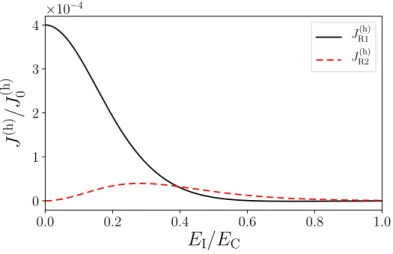
In this thesis, we will generally consider a quantum thermal machine, where the work is performed on the system, either by driving the system by an external ac supply (for example, see Chapters VIII and IX) or by means of a coupled system (for example, see Chapters IV and V where the system under study is Coulomb coupled to another system maintained at a thermal bias). In these cases, depending on the energy exchanges in the system, the details of the system, bath and coupling, the device can act as thermal machines of different sorts, for example refrigerator, thermal accelerator, heat pump, etc.
B
S
B
B S B
HM
Figure 3.1: A nanoscale system S connected to baths B. The work can be performed on the system either (left panel) by driving the system or (right panel) by coupling the system to another system (indicated by a light green shade and represented by Hamiltonian HM) through Coulomb interaction.
Now, we will discuss about different thermodynamic parameters that define the properties of a thermal machine when the system is both driven
18 thermodynamics and thermal machines: a brief review
as well as coupled to an external system. As sketched in Fig.3.1, we define the total Hamiltonian
Htot=H+HM (3.11)
where H is the Hamiltonian for the device under consideration as defined in Eq. (2.1), the system Hamiltonian, HS ⌘HS(t)is time dependent (see the
left panel of Fig.3.1), HB=ÂaHadescribes the baths (a labels the different baths) and HC=ÂaHC,adescribes the coupling between the system and the baths. HMgives the Coulomb coupled part, when the work is performed on
the system by means of a Coulomb coupled system (see the right panel of Fig.3.1).
Let’s start from the energy currents. To study the energy flux entering and exiting different parts of the device, we consider the time evolution of total Hamiltonian dhHi dt = dhHSi dt + dhHBi dt + dhHCi dt . (3.12)
The energy current entering the baths is given by
Ja(E)(t) =ih[H(t), Ha(t)]i. (3.13) The energy current flowing in the contact region is
JC,a(E)(t) =ih[H(t), HC,a(t)]i. (3.14)
And finally the energy current flowing through the system is expressed as JS(E)(t) =ih[H(t), HS(t)]i. (3.15)
On the other hand, dhHi dt = ih[Htot, H]i + ⌧ ∂HS ∂t , dhHSi dt = ih[Htot, HS]i + ⌧ ∂HS ∂t , dhHai dt = ih[H, Ha]i, dhHC,ai dt = ih[H, HC,a]i, (3.16) whereD∂HS ∂t E
=0 for static systems. We define the power developed by the
ac source as
Pac(t) =
⌧∂H
S
∂t (3.17)
and define the power introduced by coupling
PM(t) =ih[HM, HS]i. (3.18) Eq. (3.12) reduces to Pac(t) +PM(t) =JS(E)(t) +PM(t) +Pac(t) +
Â
a Ja(E)(t) +Â
a JC,a(E)(t), (3.19) where we used the fact that[Htot, H] = [HM, HS]and[Htot, HS] = [HM, HS] + [HC,a, HS]. We obtain JS(E)(t) +Â
a Ja(E)(t) +Â
a JC,a(E)(t) =0. (3.20)3.3 experiments on nanoscale quantum thermal devices 19 Upon time averaging, the heat current flowing in the contact region
JC,a(E)= 1 t Z t 0 J (E) C,a(t)dt=0, (3.21)
and the conservation of energy in the steady state is given by JS(E)+
Â
a
Ja(E)=0. (3.22)
Eqs. (3.20) and (3.22) establish the first law of thermodynamics for the nanoscale devices we will be considering in this thesis. Next we would like to define entropy(S). The power developed by ac source and the power introduced by coupling to a different system are non-conservative and hence associated with dissipation. Therefore, when the baths are kept at a tempera-ture T or have a relatively small thermal bias DT⌧T, the net rate of entropy production is given by
T ˙S=Pac+PM. (3.23)
Since both effects are dissipative in nature, Pac, PM>0 and hence ˙S>0. This
establishes the second law of thermodynamics for our quantum nanoscale devices.
3.3 experiments on nanoscale quantum thermal devices We shall start with one of the basic properties of nanoscale thermal devices: the quantum of thermal conductance. The quantization of thermal conduc-tance is analogous to the quantization of electrical conducconduc-tance in nanoscale ballistic devices at low temperature. The limit value of thermal condutance was first proposed theoretically by J. B. Pendry in 1983[36] employing the relation between entropy and the quantum limit of information flow for a finite size system in contact with a reservoir. Later, limiting value of thermal conductance given by k=p2k2BT/3h in single mode systems was observed in
a range of experimental devices: ballistic one dimensional nanostructure[37], metallic islands[38] and single electron transistor[39] to name a few.
Single electron transistors are possible setups for studying quantum prop-erties of thermal transport in nanoscale devices. The possibility of micro-fabrication has led to the realisation of metallic tunneling junctions with capacitances of the order of 10 15F. This capacitance corresponds to a
charg-ing energy (Ec) of 100µeV⇡kB⇥1.16K. So, in the sub-Kelvin temperature
regime, one would have to overcome the charging energy in order to re-alize the transport of electrons. This regime, known as Coulomb blockade regime, enables the study of single electron transport. A metallic island is characterized by the “charge state" which is defined through the num-ber of electrons (n) present in the island. Thermometry based on N-I-S tunnel junction[40] can be operated at millikelvin regime and are widely used for thermal analysis in single electron devices. Apart from thermal conductance, single electron transistors have been used to experimentally observe dissipation[41] and transport of heat[27,42] in nanoscale devices, thermoelectric coefficients[32,35], negative entropy processes[43], maxwell demon[27] and the rate of information flow[44]. Single electron transistors have also been used to engineer nanoscale thermal machines[42]. On the other hand, thermal transport has also been widely studied in photon based thermal devices. Josephson junctions and LC resonator circuits based on metal-island junctions are the basic components of these devices. Recently,
20 thermodynamics and thermal machines: a brief review
experiments based on photon based devices have led to the observation of thermal rectification[45] and quantum heat valve[46].
Thermal machines have been miniaturized down to atomic scale, utilizing cold atoms[47], colloidal particles[48,49], single molecules[50], and moreover even a single atom[51]. The recent experiments are precise up to the level of single particle transport which would have been an impossible tasks some decades back. Regarding refrigerators, absorption refrigeration was recently observed in trapped ions [52]. On a different note, quantum dot based energy harvester was recently observed experimentally by Thierschmann et al [53].
4
T H E R M A L D R A G I N C O U L O M B C O U P L E D S I N G L EE L E C T R O N S Y S T E M S
Two electrically isolated conductors placed close together can still be coupled via the Coulomb interaction. As a result, when a bias is only applied to one conductor, electronic currents can be generated in the unbiased one in such a way that a charge current is dragged in this second conductor. This phenomenon, the Coulomb drag, arises because the carriers in the two conductors are subject to a “mutual friction”, i.e. to scattering processes mediated by the Coulomb interaction between the two conductors, and can exchange momentum and/or energy. The phenomenon of drag, first proposed in 1977 by Pogrebinskii [54] in layered conductors, has so far been studied in a large variety of systems and it is still the subject of an intense research activity (see Ref. [55] for a recent review).
T + ∆T/2 V/2 T - ∆T/2 - V/2 T T 𝐽 / 𝐽 / 𝐽 / 𝐽 /
Figure 4.1: Sketch of Coulomb-coupled systems, which consists of an upper (drive) biased circuit, and a lower (drag) unbiased circuit. The conductors are represented as grey rectangles and are attached to two leads each. The two conductors are coupled only through the Coulomb interaction. As indicated by the black arrows, the sign of charge and heat currents is positive when they enter an electrode.
So far most of the attention has been devoted to the effect of drag on the charge current. More recently, the drag of charge between zero-dimensional systems have been theoretically considered for single-level Quantum Dots (QDs) in Refs. [56,57,58,59]. Experimental investigations in systems com-posed of two capacitively coupled QDs are reported in Ref. [60] (emphasizing the importance of co-tunneling processes [58]) and in Refs. [61,62] for the case of graphene-based QDs. The drag of charge in coupled double QDs sys-tems has been also experimentally addressed in Ref. [63]. In addition, energy harvesting from thermal and voltage fluctuations in coupled QDs systems at-tached to three terminals has been considered theoretically [64,65,66,67,35] and experimentally [68,69,70,71].
Another consequence of the Coulomb coupling between two nearby con-ductors is the fact that a flow of heat can also be induced in the unbiased
22 thermal drag in coulomb coupled single electron systems
conductor. This phenomenon, which is distinguished from the drag of charge that is constrained by the charge conservation within individual conduc-tors, has been hardly considered in the literature so far [72]. In the case of metallic islands, heat currents can be induced in the unbiased circuit as a result of energy transfer, through the capacitive coupling, from the upper island. Such energy transfer has been recently considered for the implemen-tation of a heat diode [73], of a minimal self-contained quantum refrigeration machine [74], of a three-terminal QD refrigerator [75], of an autonomous Maxwell demon [76], of a Szilard engine [27], of a nanoscale thermocouple heat engine [72], and for the study of a correlation-induced in SINIS refriger-ator [77]. In this chapter we will investigate another important case of this kind, thermal drag.
The setup we consider is represented in Fig.4.1. Two mesoscopic conduc-tors, represented by grey rectangles, are coupled through Coulomb inter-actions, but cannot exchange electrons. One conductor is contained in the upper (drive) circuit, which is either voltage or thermal biased, while the other conductor is part of the lower (drag) circuit, which is unbiased. As specified in Fig.4.1, the left (right) electrode in the drive circuit is kept at a voltage±V/2 and temperature T±DT/2, while the electrodes in the drag circuit are kept at the same temperature T and at zero voltage. Our goal is to study the general properties of the heat currents flowing in the drag circuit, IL2(h)and IR2(h), as a result of energy transfer between upper and lower circuits, due to Coulomb interaction.
We define the drag currents as
Jdrag(c/h)= J (c/h)
L2 JR2(c/h)
2 , (4.1)
where JL2(c) and JR2(c) are charge currents in the drag circuit. Notice that the charge current is conserved separately on the upper and lower circuit (JL1(c)+
JR1(c)=0 and JL2(c)+JR2(c)=0, respectively). We will focus on the following two
cases:
i) A pair of capacitively-coupled metallic islands in the Coulomb block-ade regime
ii) A pair of capacitively-coupled quantum dots in the Coulomb blockade regime.
Regarding system i) and ii), we study the general properties of the dragged heat using a master equation approach up to second order tunnelling events (co-tunneling)[78]. We find that the dragged heat current Jdrag(h) is finite, even in the cases where the dragged charge vanishes (i. e. when the island-electrode couplings are energy-independent). We study the behavior of the dragged heat current, driven by either a voltage bias V or a thermal bias DT, as a function of the various parameters characterizing the system, such as the gate voltages and the capacitive coupling CI between the islands. We
find, in particular, that Jdrag(h) exhibits a maximum as a function of CI. By
expanding the dragged heat current for small values of V or DT, we find analytic expressions for Jdrag(h) which result quadratic in V or DT. We find, moreover, that co-tunneling events yield an important impact on the dragged
4.1 thermal drag in coulomb coupled metallic islands 23 heat current, though not changing the quadratic dependence on V or DT. Finally, we find that the behavior of the dragged heat current can change qualitatively if one replaces one of the electrodes in the drag circuit with a superconductor. More precisely, under appropriate conditions we find that heat can be extracted from the normal electrode in the drag circuit (JL2(h) <0). Additionally, the superconductor allows a finite dragged charge current whose sign can be controlled by the gate voltages.
As far as system ii) is concerned, we find similar dependence of the drag heat current on the thermal or potential bias as in system i). However, in the case of QDs, the energy filtering mechanism can be made more efficient. We observe a significant heat flow from one bath to another in the drag when one of the system-bath coupling in the drag is made energy dependent.
The chapter is organized as follows: In the next Section we will discuss the case i) in which the thermal drag occurs in the case of two coupled metallic islands. We will consider the contribution to the drag due to sequential tunneling and co-tunneling. In Section4.2we move to consider the second setup of Coulomb coupled quantum dots.
4.1 thermal drag in coulomb coupled metallic islands The first system considered, depicted in Fig. 4.2, consists of two metallic islands (labeled 1 and 2), each one tunnel-coupled to two electrodes and capacitively-coupled to a gate kept at a voltage Vgi, with i=1, 2. Ca is the capacitance andRais the resistance associated to the tunnel junction between lead a=Li, Ri and the island i, while Cgiis the capacitance associated to the
gate. The two metallic islands (assumed to be at equilibrium temperature T) are coupled through a capacitance CI, which does not allow electron
transfer. We assume that all capacitances are small so that the charging energies relevant for transport (see below) are the largest energy scales in the system and the islands are in the Coulomb blockade regime. Single electron tunneling processes in each metallic island, thus, are associated to an increase or decrease in the electrostatic energy of the system, which is given by
EU(n1, n2) =EC,1(n1 nx1)2+EC,2(n2 nx2)2+ +EI(n1 nx1) (n2 nx2).
(4.2) Here n1and n2represent the number of electrons present on island 1 and
2, respectively. EC,i = e2/(2Ci) is the charging energy of island i (where
Ci = CLi+CRi+Cgi+CI,i, with CI,11 = ˜C21+CI 1, CI,21 = ˜C11+CI 1 and
˜Ci = CLi+CRi+Cgi) and EI is the inter-island interaction energy given
by EI = e2(C˜1+C˜2+C˜1C˜2/CI) 1. The symbols nx1and nx2 represent the
“external charges” determined by the gate potentials, Vg1and Vg2respectively,
and dependent on the voltage bias V as
nx1= V/2 CL1 V/2 Ce R1+Vg1Cg1 (4.3)
and
nx2= Vg2eCg2. (4.4)
For the sake of simplicity, we will assume that Cg1=Cg2 ⌘Cgand that all
the capacitances relative to the tunnel junctions are equal, namely CL1 =
CR1 = CL2 = CR2, so that C1 = C2 ⌘ C and we can define the charging
energy EC =e2/(2C). Note that nx1becomes independent of V and takes
24 thermal drag in coulomb coupled single electron systems CI 1 2 CR1 CL1 CR2 CL2 Cg1 Cg2 R1 L1 R2 L2 Vg1 Vg2
Figure 4.2: Sketch of the first system under consideration composed of two capacitively-coupled metallic islands labeled by 1 (in the drive circuit) and 2 (in the drag circuit). L1, L2, R1 and R2 labels the four electrodes which are tunnel-coupled to the islands.
Charge Ja(c)and heat Ja(h) currents can be expressed in terms of the proba-bility for the occupation of the islands, and the transition rates for electrons to be exchanged between the islands and an electrodes. The actual expressions for the currents depend on whether one has to account for only first order tunneling processes (sequential tunneling regime) or second order processes have to be considered too (co-tunneling). The probability p(n1, n2)for the
occupation of island 1 with n1 electrons and island 2 with n2 electrons is
determined through a set of master equations (see App.D) which accounts for all possible tunneling processes in the system.
4.1.1 Sequential tunneling regime
Within the sequential tunneling regime, we have that the charge and heat currents in the lower circuit take the form
Ja(c/h)=Q(c/h) h G(c/h)a,2 (n1, n2)p(n1, n2) +G(c/h)a,2 (n1+1, n2)p(n1+1, n2) G2,a(c/h)(n1, n2)p(n1, n2+1) G(c/h)2,a (n1+1, n2)p(n1+1, n2+1) i , (4.5) respectively, where a =L2, R2 and Q(c) =e, Q(h) =1. We have assumed
small temperatures and biases so that only four charge states contribute to transport, namely(n1, n2),(n1+1, n2),(n1, n2+1)and(n1+1, n2+1).
In Eq. (4.5), G(c/h)a,i (n1, n2)is the particle/heat transition rate for an electron
to reach island i from lead a [with the island initially in the state(n1, n2)],
and G(c/h)i,a (n1, n2)is the particle/heat transition rate for an electron leaving
island i to reach lead a [with the island in the final state(n1, n2)]. As long
as the energy-dependence of the lead-island couplings1can be disregarded (see Sec.4.1.3, where this assumption will be lifted), the particle and heat transition rates can be written as
G(c/h)a,i (n1, n2) = e21 RaF
(c/h)
ai [dEUi(n1, n2) eVa], (4.6)
1 Lead-island couplings are energy-dependent when their tunnelling matrix elements depend on energy or when at least one density of states (of the lead or of the island) depend on energy.