Alma Mater Studiorum · Università di Bologna
School of Science
Department of Physics and Astronomy Master Degree in Physics
Digital quantum simulations
of Yang-Mills lattice gauge theories
Supervisore:
Prof. Elisa Ercolessi
Co-Supervisor:
Dott. Sunny Pradhan
Submitted by:
Luca Lumia
Sommario
I metodi di calcolo tradizionali per le teorie di gauge su reticolo risultano problematici in regioni di diagrammi di fase a grandi valori del potenziale chimico o quando sono utilizzate per riprodurre la dinamica in tempo reale di un modello. Tali problemi possono essere evitati da simulazioni quanti-stiche delle teorie di gauge su reticolo, le quali stanno diventando sempre più riproducibili sperimentalmente, grazie ai recenti progressi tecnologici. In questa tesi formuliamo una versione delle teorie di Yang-Mills su reticolo ap-propriata per risolvere il problema della dimensione infinita dello spazio di Hilbert associato ai bosoni di gauge. Questa formulazione è adatta per esse-re riprodotta in un simulatoesse-re quantistico e ne implementiamo una completa simulazione su un computer quantistico digitale, sfruttando il framework Qi-skit. In questa simulazione misuriamo le energie del ground state e i valori di aspettazione di alcuni Wilson loop al variare dell’accoppiamento della teoria, per studiarne le fasi e valutare la prestazione dei metodi usati.
Abstract
The standard computational tools for lattice gauge theories encounter prob-lems in regions of phase diagrams with large chemical potentials or when they are used to reproduce the real-time dynamics of a model. These issues can be avoided by performing quantum simulations of lattice gauge theories, which are becoming experimentally realizable thanks to recent technological advancements. In this thesis we formulate on a lattice a suitable version of Yang-Mills theories that solves the problem of the infinite dimensionality of the Hilbert space associated with the gauge bosons. This model is suited to be realized on a quantum simulator and we implement the full simulation on a digital quantum computer within the Qiskit framework. The ground state energy and the expectation values of some Wilson loops have been measured at several values of the coupling of the theory, in order to study its phases and to test the performance of our methods.
Contents
Introduction 7
1 Yang-Mills theory on a lattice 13
1.1 Continuum Yang-Mills theory . . . 13
1.2 Lattice regularization . . . 16
1.3 Parallel transport and Wilson loops . . . 18
1.4 Gauge fields on a lattice . . . 21
1.5 Hamiltonian Yang-Mills theory . . . 24
1.6 The Kogut-Susskind hamiltonian . . . 27
1.7 Phase structure of gauge theories . . . 33
2 Quantum simulations for lattice gauge theories 37 2.1 Analog and digital simulations . . . 37
2.2 First step: encoding . . . 40
2.3 Second step: time evolution . . . 41
2.4 Third step: measurements . . . 43
2.5 Simulating lattice gauge theories . . . 46
2.5.1 Hilbert space truncation . . . 46
2.5.2 Gauge fields integration . . . 48
2.5.3 Quantum link models . . . 51
2.5.4 Finite group approximation . . . 52
3 Simulating a general finite group LGT 55 3.1 Hamiltonian for a finite gauge group . . . 56
3.1.1 Geometric interpretation of the hamiltonian . . . 56
3.1.2 The representation basis . . . 57
3.1.3 The finite group electric term . . . 60
3.2 Duality and generalized Fourier transforms . . . 62
3.3 Time evolution algorithm . . . 68 3
4 Zn gauge models 73
4.1 Pure Zn lattice hamiltonian . . . 73
4.2 Ising gauge theory . . . 75
4.2.1 Formulations of the model . . . 75
4.2.2 Structure of the Hilbert space . . . 77
4.2.3 The Z2 confined phase . . . 79
4.2.4 The Z2 deconfined phase . . . 81
4.2.5 Boundary conditions and the Z2 topological fluid . . . 83
5 Implementation of the quantum algorithm 87 5.1 The gate-set for Z2 . . . 87
5.2 Preparation of the initial state . . . 90
5.3 Measurement of physical observables . . . 94
5.4 Implementation and results . . . 97
Conclusions and perspectives 105 A The mathematical toolbox: groups and representations 109 A.1 Fourier analysis on finite groups . . . 109
A.2 Fourier analysis on compact Lie groups . . . 114
A.3 Riemannian structure on Lie groups . . . 115
B The computational toolbox: quantum codes and Qiskit 119
Introduction
The concept of gauge symmetry lies at the heart of our current understanding of many fundamental phenomena in nature, touching fields from condensed matter to high-energy physics. It was first introduced as an intrinsic re-dundancy in the description of the classical electromagnetic field through its potential Aµ = ( , ~A ): different potential functions (x), ~A(x) generate to
the same electric and magnetic fields ~E(x), ~B(x)if they are related by a par-ticular relation called “gauge transformation”. Hence, we have the freedom to choose different configurations that describe the same physical state. Gauge freedom is not an actual symmetry, nevertheless it strongly constraints the structure and the properties that the theory should have. For instance, in QED it has the key role of forbidding unitarity violations [65].
The gauge symmetry of QED can be constructed by promoting the global U(1) electric charge symmetry to a local one. Similarly also the other two fundamental interactions of the Standard Model of particle physics are for-mulated as Yang-Mills gauge theories, which can be seen as a generalization of QED to arbitrary non-abelian gauge groups, and gauge symmetries play an essential role also in the Higgs mechanism, which generates the mass of all fundamental particles. Besides the electroweak and strong interactions, also gravity can be thought of as a gauge theory, since when it is made local, the global Poincaré symmetry can lead to the diffeomorphism invariance typical of general relativity, even though some subtleties are involved [11].
Stepping aside from high-energy physics, gauge symmetries are important also in condensed matter models [29]. The simplest way to introduce them is to modify the Ising model in such a way that its Z2 symmetry becomes local,
leading to a very interesting model that cannot magnetize but still shows a phase transition. Gauge symmetry is useful also to describe phenomena like superconductivity (whose explanation inspired the development of the Higgs mechanism), or to characterize topological phases like fractional quantum Hall effect states, which can be described as a Chern-Simons theory. In spite of their very constrained formulation, the behaviour of gauge theories is extremely rich, giving shape to the multi-colored variety of phenomena
that we observe in nature. This makes it extremely challenging to solve their dynamics from first principles and several approaches were tried. In continuum quantum field theory, interacting models are typically treated with perturbative expansions on the coupling constant, only meaningful as long as the coupling constant is small. However, it is well known that the physical couplings are not actually constants, but they run with the energy scale of the process under consideration. For Quantum Electrodynamics, the coupling constant (electric charge) is weak for low energies and the large scale electromagnetic phenomena that we observe can be treated with perturbation theory. Increasing the energy, the coupling constant grows and this effect can be interpreted in a very clear way as the screening of the electric charge due to a progressive production of virtual electron-positron dipoles. This interpretation is sensible until the energy scale of ⇤QED = 10286 eV where
QED has a Landau pole and the coupling constant diverges, meaning that perturbation theory has to break down at a scale ⇤ < ⇤QED[65]. Nonetheless,
for QED the Landau pole is not an actual phenomenological problem, since 10286 eV is a huge scale, far larger than Planck’s mass, and we already expect
something else to appear and change the physics before.
The same cannot be said for Quantum Chromodynamics, the SU(3) gauge theory describing the strong interaction between quarks. QCD is asymptoti-cally free and the strong coupling vanishes when the energy scale is pushed to infinity; therefore, for small distance/high-energy processes, the coupling constant is finite but small and calculations can be done using perturbation theory. Instead, low energy QCD is characterized by a large coupling con-stant which diverges at a scale ⇤QCD ⇡ 300 MeV [65]. Unlike for QED, this
is now a matter of concern: perturbation theory loses its meaning roughly at the scale of the mass of the hadrons, signaling that the degrees of freedom that we use to formulate small distance QCD probably are not best suited to describe large distance strong phenomena. One possibility could be to use effective field theories where the hadrons become the fundamental degrees of freedom, otherwise, we should find alternative non-perturbative approaches. QCD is formulated in terms of quarks. The success of the quark con-stituent picture of hadrons, both for the interpretation of the systematics of their static properties and for the description of their dynamics, has always made very difficult to believe that quarks do not exist, even though they have never been seen as isolated fractional charges. This suggests the exis-tence of a confinement mechanism, that prevents quarks from appearing as separate particles in a final state. Whatever non-perturbative approach we choose, we should take into account that confinement has to be explained somehow. The most important non-perturbative approach is probably lat-tice QCD, first studied by Ken Wilson in 1974 [90], in an paper where he
Contents 9
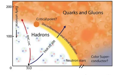
Figure 1: The proposed form of the QCD phase diagram, drawn with
respect to the chemical potential on the x axis and the temperature on the y axis, both in MeV. This image is taken from [72].
introduced a hypercubic spacetime lattice as a gauge-invariant regulator of the ultraviolet divergences, with quark fields living on the lattice sites and gluons residing on the links between the nearest neighbour sites. If we work on a Wick-rotated euclidean spacetime and if we discretize it by formulating the theory on a lattice, QCD becomes a typical model of statistical mechan-ics. Wilson showed analytically that lattice QCD exhibits confinement in its strong coupling limit, suggesting also that it should be a phase transition what distinguishes the confined and deconfined regions of QCD. In addition to that, thanks to the connection between lattice gauge theories and sta-tistical mechanics, particle physics profited enormously from the numerical methods used for condensed matter systems, such as Monte Carlo algorithms [32]. This approach made numerically accessible to classical computers sev-eral important quantities, such as masses and matrix elements of baryons and mesons, or properties at thermal equilibrium of the quark-gluon plasma, which is a phase of QCD that we expect to take place at sufficiently high temperatures and large values of the chemical potential.
The phase structure of QCD is not completely understood yet, either theoretically or experimentally, but it is suspected to resemble the phase diagram reported in Fig. 1. Close to the origin of the (T, µ) plane, we expect a hadronic phase, where quarks are confined and the relevant degrees of freedom are the hadrons. Increasing the temperatures, while keeping low values of the chemical potentials, we expect to get a gas of hadrons until we enter the quark-gluon plasma phase, where the relevant degrees of freedom
are well-separated deconfined quarks, antiquarks and gluons, forming the so-called “quark matter”. Another form of quark matter is present in the colour-flavour locked phase, expected at ultra high-density regions, where quarks should show a colour-superconducting behaviour. Regions with high temperatures and small densities can be explored with high-energy hadron collisions, such as the ones studied with the ALICE experiment at LHC, whereas regions with high densities and lower temperatures might correspond to the phases of matter contained in the core of neutron stars. We expect the hadronic-confined and the quark matter-deconfined phases to be separated by a critical line along which there is the spontaneous symmetry breaking of the chiral symmetry. In the hadronic phase the chiral symmetry should break, because an unbroken (although approximate, since the quarks u and d are not exactly massless) symmetry is not compatible with the huge mass difference that we measure between parity partners such as the nucleon N with mN = 940 MeV and N⇤ with mN⇤ = 1535 MeV [32].
Monte Carlo calculations led to great results, but they are not able to explore the whole QCD phase diagram, since at high density regions the large values of the chemical potential cause the famous sign problem. We are typically interested in computing sums over configurations of the form
hA i = R
D A( ) e S( )
R
D e S( ) ,
where A is some observable and a generic variable encoding the configu-ration. Sweeping over the whole configuration space with D would be a computationally intensive operation and usually one relies on Monte Carlo importance sampling methods [1]: as long as the measure e S is positive
defi-nite, it can be interpreted as a probability distribution and we can simplifying the sum by considering only the most relevant contributions. However, this is the situation only at µ = 0, since when a chemical potential is added the euclidean action becomes in general a complex number, which can be highly oscillating. In this regime, importance sampling algorithms fail because e S
cannot be interpreted as a probability and, in general, the near-cancellations of positive and negative contributions to the integral introduce large errors in numerical methods. In addition to that, trying to reproduce the real-time dynamics has a similar kind of bottleneck, so that also out of equilibrium properties are hard to obtain using this approach [64].
The same issues arise in condensed matter systems and researchers started to study different approaches to tackle them. However it has been shown [87] that a general solution of the sign problem is NP-hard, meaning that any other NP problem can be mapped into it, so that a polynomial solution of
Contents 11 the sign problem would automatically provide a polynomial solution for all NP problems, therefore implying that P=NP. This is clearly a difficult task, so the attention was drawn by different methods and some of them were borrowed from the field of quantum information. The idea is to simulate quantum models with algorithms specifically tailored to encode the quantum properties of the system under attention. They usually require the theory to be formulated in the hamiltonian formalism (which is automatically free of the aforementioned sign problems) and, given an appropriate initial state | (0)i, they aim to simulate its time evolution | (t)i = e iHt| (0)i. However,
when implemented on a classical computer, they meet the problem of the explosion of the dimension of the Hilbert space. A quantum system of 40 spins |s = ±1/2i has 240 independent states and its hamiltonian will be
represented by a 240⇥ 240 matrix, which occupies 4 TB of memory by itself.
Being the growth exponential, small increases of the number of lattice sites are enough to exceed the computational capabilities of even the most powerful supercomputers. Currently, the most common approach aims to optimize the computation on a classical computer, for instance by using particularly efficient algorithms like the DMRG (density matrix renormalization group) [8], or by exploiting the symmetries of the model to restrict its dynamics (and consequently the computation) to the physical Hilbert space, using e.g. a tensor network representation [57] of the gauge-invariant states.
A natural solution to this problem was proposed by Richard Feynman in 1982 [24], who suggested that we should use a quantum simulator to repro-duce the behaviour of another quantum system, since only a truly quantum device might be able to encode all the quantum properties of the system under interest. Another advantage of quantum simulations is that many standard proposal using the DMRG and tensor networks are suited for 1d models and their generalization in other dimensions is far form trivial, whereas in principle the simulation approach can be employed in any dimension.
Today we have reached the technology sufficient to realize such quantum simulators: there are condensed matter systems, such as ultra-cold matter on optical lattices, superconducting qubits, nuclear spins or photon systems, whose interactions can be engineered with the freedom sufficient to represent wide classes of hamiltonians. The recent technological advancements fueled a vigorous interest on the topic and several projects have been proposed and re-alized by pioneering experiments with analog simulators. For instance, ultra-cold Fermi gases in optical superlattices can be used as quantum simulators of relativistic fermions on a D=3+1 lattice, allowing to realize a simulation of a 3d topological insulator [10] or to reproduce fractional quantum Hall states and non abelian anyons [35]. Cold atoms may be used to test also exactly solvable theories like the Thirring model or the Gross-Noveau model, that
can be used as a benchmark to demonstrate the ability of these simulators to reproduce important dynamical phenomena [15]. Another example is [93], where cold atoms are used to enforce gauge symmetry by taking advantage of the angular momentum conservation. These are only a few of many recent works of the field [8]: quantum simulations are becoming increasingly feasible and the number of proposals is growing. One could also try to encode the dy-namics of a condensed matter system on digital quantum computers, which are still at a first development stage, but they are experiencing extremely fast improvements. Quantum computers are supposed to be universal, meaning that they have the potential of being able to reproduce the dynamics of any quantum system through purely digital methods.
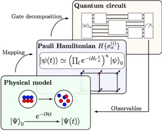
The present thesis fits into this context, aiming to study a general method to simulate lattice gauge theories on a digital quantum computer and to im-plement a simple example. The simulation of lattice gauge theories using digital quantum computers is a young field of research and there are only a few studies in this direction, such as [21, 54, 56, 77]. Therefore this thesis is not meant to observe new physics, but rather our aim is to make a prelimi-nary analysis of the performances of the methods we propose and to find out how to improve them, which is relevant since their generality suggests that one day they might be used to simulate any lattice gauge theory. We shall start by quickly discussing in Chapter 1 Yang-Mills theories in the continuum, putting our emphasis on the objects of primary importance when the theory is placed on a lattice. The general construction of a lattice gauge theory is explained both in the path integral formalism and in the hamiltonian for-malism, which is crucial for the implementation of the theory on a quantum simulator. In Chapter 2 we move to the description of the general structure of quantum simulations and the problems that can be met when implement-ing one as well as some common approaches used to overcome them, before focusing on the finite group approximation for the rest of the thesis. Chap-ter 3 describes a possible definition of a hamitonian for a finite group lattice theory, relying on the mathematical structure of the well established theory for continuous gauge groups, and presents a quantum algorithm able to sim-ulate the corresponding time evolution for an arbitrary gauge group. Finally we focus on Zn lattice gauge theories, outlining their general behaviour in
Chapter 4 and describing in Chapter 5 the implementation of our simulation of a pure Z2 model as well as its results.
CHAPTER
I.
Yang-Mills theory on a lattice
The Standard Model of particle physics is based upon the formulation of gauge theories first given by Chen Nin Yang and Robert Mills in 1954 [?], who extended the local U(1) symmetry of QED to the non abelian group SU(2) in an attempt to describe the strong interactions in atomic nuclei as a consequence of a local isospin symmetry. Their work can be directly general-ized to any non abelian group, allowing to formulate the SU(2)L and SU(3)C
theories that describe weak and strong interactions. Quantum field theories are formulated in terms of continuous fields on a continuous spacetime, but if we want to reproduce them on any kind of computer, classical or quantum, we ought to discretize them, since computers have finite memory resources and an infinite amount of information cannot be represented. In this way, we get to a theory defined on a discrete lattice, ideally large but still finite. Lattice gauge theories, and in particular lattice QCD, were one of the first non perturbative approaches introduced to study properties such as quark confinement. This chapter aims at introducing lattice Yang-Mills theory and more specifically their hamiltonian formulation, which is fundamental for quantum simulations. We start by describing the continuum Yang-Mills theory, in order to set the notation and to underline some key points and then we give the standard path integral description of lattice gauge theories, before moving on to their hamiltonian formulation.
1.1 Continuum Yang-Mills theory
QED describes the interactions between a charged Dirac spinor and the electromagnetic field Aµ where the interaction term is given by the minimal
coupling, which can be interpreted in a geometrical setting by introducing the U(1) covariant derivative Dµ = @µ iAµ [65]. A similar theory can be
constructed with different matter fields, such as complex scalars. Yang-Mills theories are defined by the choice of the gauge group G, usually supposed to be a compact Lie group, and by the choice of the matter fields plus the representation of G they belong to. Keeping in mind the example of QCD, we take G = SU(N) and matter made of Dirac spinors in the fundamental representation. The gauge fields Aµ are elements of the Lie algebra g =
su(N) and can be expanded as Aµ = AaµTa, if we introduce a set {Ta},
a = 1, . . . ,dim G of hermitian generators of su(N), usually chosen to satisfy
[Ta, Tb] = i fabcTc (1.1)
tr (TaTb) =
1
2 ab, (1.2)
where fabc are the completely anti-symmetric structure constants of SU(N).
In these formulas we are employing Einstein’s summation convention over re-peated indices. If we take the Minkowski metric with signature (+, , . . . , ), the action of the free matter field in D = d + 1 dimensions is
S0[ , ¯ ] =
Z
dd+1x ¯ (i/@ m) (1.3)
and it is invariant under global transformations (x) 7! g (x), where g is any element of the gauge group SU(N). The symmetry can be promoted to local if we introduce the gauge field Aµ, interacting with the matter field
according to the Yang-Mills action SY M[A, , ¯ ] =
Z
dd+1x ¯ (i /D m) 1
2g2tr (Fµ⌫F
µ⌫) , (1.4)
where the covariant derivative is Dµ = @µ iAµ and the associated
curvature tensor, also called field strength tensor, is
Fµ⌫ = i [Dµ, D⌫] = @µA⌫ @⌫Aµ i [Aµ, A⌫] = Fµ⌫aTa. (1.5)
The symmetry is local, i.e. if we define a function g(x) : M ! SU(N) on the spacetime M, the simultaneous transformations
(x) 7! g(x) (x) (1.6)
Aµ(x) 7! g(x)Aµ(x)g(x) 1 + ig(x)@µg(x) 1 (1.7)
leave SY M invariant, as Dµ (x) ! g(x)Dµ (x) and Fµ⌫ 7! g(x)Fµ⌫g(x) 1
so that, thanks to the ciclicity of the trace, SY M 7! S 0
Y M = SY M. One
should keep in mind that we are being a little sloppy here: since the group elements do not act directly on but only through the chosen representation
1.1. Continuum Yang-Mills theory 15 ⇢, we should have written ⇢(g(x)) (x). For instance, if the matter field is , belonging to the adjoint representation, the covariant derivative becomes Dµ = @µ i[Aµ, ]. An equivalent formulation can be given by rescaling
Aµ ! ˜Aµ = Aµ/g, so that Dµ = @µ ig ˜Aµ and ˜Fµ⌫ = Fµ⌫/g = @µA˜⌫
@⌫A˜µ ig [ ˜Aµ, ˜A⌫]; the kinetic term for ˜Aµ becomes 1/2g2tr Fµ⌫Fµ⌫ =
1/2tr ˜Fµ⌫F˜µ⌫. In the following developments it will be convenient to split
Fµ⌫ into the chromoelectric field Ei = F0i, Ei = EiaTa and into the
chro-momagnetic field Bi = 1 2✏
ijkF
jk, Bi = BiaTa. ~E and ~B are 3d objects so
we take Ei = E
i, Bi = Bi even though Ai = Ai. The quantization of the
theory is commonly performed in the path integral formalism, where Z =
Z
DAD ¯ D ei S[A, , ¯ ] (1.8)
is the naive path integral. In the continuum formulation it is divergent as a result of the integration on the infinite redundant degrees of freedom [65] and it has to be taken care of using the Faddeev-Popov procedure and BRST quantization . On a lattice instead, the gauge redundancy does not pose a threat to the finiteness of Z [58], since the integral will be performed on the elements of the gauge group, which is compact, in place of the elements Aµ
of the Lie algebra, that is an unbounded vector space.
This was a recap of the formulation of Yang-Mills theories on Minkowksi spacetime, however, lattice theories are often formulated on a euclidean spacetime. There are mainly two reasons for choosing to do so. One is that the Feynman’s weight eiS is mapped to a Boltzmann’s weight e SE,
whose damped behaviour is easier to handle than the oscillations of eiS and
allows to exploit the traditional Monte Carlo methods. The second reason is that minkowskian quantum field theories have to be Lorentz invariant, but the non-compactness of SO(1,3) causes the residual symmetry to lose any remnant of the boosts [86]. Instead, SO(4) is a compact group and this symmetry of the euclidean theories leaves a well behaved discrete symmetry subgroup after the reduction of the continuous spacetime to a lattice.
In order to get the euclidean formulation, we have to analytically extend x0 to imaginary times. The usual Wick rotation x0 ! ixD implies that a
minkowskian action SM transforms according to
i SM ! SE , (1.9)
where the euclidean action SE represents the energy of the system. If we
consider e.g. D=4, since d4x
SE = Z d4xE LE (1.10) i SM = i Z d4xM LM ! Z d4xE LM = SE (1.11)
and we can identify the euclidean lagrangian with LM ! LE. A vector
field is supposed to transform consistently with @/@xµ
M, so the time
compo-nent of the euclidean vector field AE
µ is defined as AM0 ! i AE4. Substituting
it into the definition of the field strength tensor, we get FM
0k ! i F4kE, so that
the gauge part of the lagrangian transforms as LM 1 2g2tr (F M µ⌫F µ⌫ M ) ! 1 2g2tr (F E µ⌫F µ⌫ E )⇢ LE. (1.12)
Of course the euclidean objects do not distinguish between up and down indices and we have raised them only for aesthetic reasons. The matter part of the lagrangian contains spinors and we have to make use of euclidean Dirac matrices, which satisfy a euclidean Clifford algebra
{ Eµ, E⌫} = 2 µ⌫. (1.13)
Since LM (i¯ Mµ @µ+ MµAµM m) and i M0 @0 ! M0 @4, we choose 4
E = M0 , Ek = i Mk , (1.14)
so that i µ
M@µ! Eµ@µ and i Mµ ! i µ
EAEµ and together they yield
LM (i¯ Mµ@µ+ MµAMµ m) ! (¯ µ
E@µ i EµAEµ + m) . (1.15)
Then, if we set DE
µ = @µ iAEµ and if we recall that LM ! LE, the
euclidean Yang-Mills lagrangian can be identified with
LE = 1 2g2tr F E µ⌫F µ⌫ E + ¯ ( µ EDEµ + m) . (1.16)
1.2 Lattice regularization
Quantum field theories are disseminated of divergent integrals and the run-ning of the parameters made necessary by renormalization calculations may cause perturbation theory to break down at some regimes, where a
non-per-1.2. Lattice regularization 17 turbative approach is needed [32]. We choose to discretize the spacetime by formulating the theory on a hypercubic oriented lattice
⇤ =nx2 M x = D X µ=1 nµaˆµ , nµ= 0, 1, . . . , Lµ 1 o ,
where a is the spacing, ˆµ is a unit vector in the µ direction and Lµ is the
extension of the lattice along µ. Let f be a function on ⇤. The discretized version of the integral clearly is
Z
M
dDx ! aD X
x2 ⇤
, (1.17)
then we can define the lattice Fourier transform of f as ˜
f (p) = aD X
x2 ⇤
e ip·xf (x) . (1.18)
If we put periodic boundary conditions f(x + aˆµLµ) = f (x), we want the
plane waves e ip·x to satisfy the same requirement [73]. This selects the set
of allowed values for pµ, which is the reciprocal lattice
˜ ⇤ =np2 RD p µ = 2⇡ aLµ kµ, kµ= Lµ 2 + 1, . . . , Lµ 2 o .
Denoting the size of the lattice with |⇤| = L1· ... · LD, the previously defined
Fourier transform can be inverted with the following formula:
f (x) = 1
aD|⇤|
X
p2 ˜⇤
eip·xf (p) .˜ (1.19)
All momenta can be restricted to the first Brillouin zone, therefore the pres-ence of the lattice introduces a finite momentum cut-off, which regulates the divergences of the theory. We can discretize also @µ as
µf (x) =
f (x + aˆµ) f (x)
a . (1.20)
This is the lattice forward derivative; a backward derivative can be analo-gously defined [58]. When we discretize the spacetime, any field (x) should correspondingly get restricted to the lattice. Let us consider a scalar field to begin with. The dynamics of the lattice field should be governed by a prop-erly discretized action; suppose that the continuum action for in D = 4 dimensions takes the standard form
S[ ] = Z d4x 1 2 @µ (x) 2 + V (x) . (1.21)
Then, if we assume that the lattice field (x) is defined on the lattice sites x2 ⇤ (as we are going to see in section 1.4, this assumption is correct only for matter fields), the naive discretization of S[ ] provides
S[{ (x)}] = a4 X x2 ⇤ 1 2 4 X µ=1 ✓ (x + aˆµ) (x) a ◆2 + V (x) . (1.22)
This naive lattice action can be considered correct only when is a scalar field, because also fermions are problematic [58]. If we are interested in the low-energy physics of the model, we can limit ourselves to consider
V( ) = m0 2
2+ 0
4!
4 (1.23)
since all the other terms allowed by the symmetries are irrelevant in the sense of the RG flow [86]. Once the action is chosen, the euclidean path integral on the lattice can be defined as follows
Z = Z D e S[ ] ⌘Z ✓ Y x2 ⇤ d (x) ◆ e S[{ (x)}]. (1.24) It has the form of a partition function for a model of statistical mechanics, whose configuration is defined by the values of field { (x)}, playing the role of one component real “spins” attached to each site x 2 ⇤. The path integral can be used to compute any correlation function. In particular, the 2-point correlator falls off exponentially within a scale given by the correlation length ⇠, which is related to the mass gap m = E1 E0 of the theory as [46]
m = 1
⇠ a. (1.25)
Consequently an interesting continuum limit a ! 0 with a finite mass spec-trum can only be found when ⇠ ! 1, i.e. at a critical point. It is, therefore, crucial to study the phase diagram of lattice theories and the nature of their critical regions.
1.3 Parallel transport and Wilson loops
Before we describe the discretization procedure for the Yang-Mills field, it is convenient to pause and define some objects that will be crucial in the devel-opment of this thesis. Generally speaking, in order to “feel” gauge transfor-mations, matter fields must have some internal degrees of freedom belonging
1.3. Parallel transport and Wilson loops 19 to a vector space V on which the gauge fields act through a representation ⇢ :G ! GL(V). For instance, the quark fields of QCD are functions
q : M ! C3 ⌦ C4 , q(x) = 0 @qqRG(x)(x) qB(x) 1 A .
where each qa(x)is a Dirac spinor belonging to C4. Here, the internal space of
the chromoelectric charge is V = C3, where the fundamental representation
of SU(3) acts. The dynamics of these objects is governed by a covariant derivative, which, as it is well known in differential geometry, is related to a notion of parallel transport: it tells us how a chromoelectric charge vector
~
w2 V rotates when we drag it along a path on the spacetime M.
Mathematically speaking, this parallel transport is defined on a vector bundle E which locally looks like E ⇠ M ⇥ V and the quark fields q(x) can be seen as local sections of E [6] (neglecting the C4 part of spinors, which
has no relevance here). The covariant derivative Dµ= @µ iAµ
is the structure that we need to differentiate local sections on a fiber bundle. Being Aµ= AaµTa2 g, under the representation ⇢ to whom matters belongs,
Aµ is realized as a matrix Aµji belonging to End(V)
Aµ= AaµTa d⇢
! Aµji = Aaµ(Ta)ij.
Let {~ej} be a basis for V. The Christoffel symbols for Dµ are given by
Dµ~ej = iAµji ~ei (1.26)
Suppose that we want to drag a vector ~w 2 V, defined a point xi 2 M,
along the path (⌧) , ⌧ 2 [⌧i, ⌧f] s.t. (⌧i) = xi. The resulting vectors are
found by imposing that their covariant derivatives along the tangent vector v(⌧ ) = 0(⌧ ) vanish, meaning that they are parallel transported. Expanding
the covariant derivative on the bases ~w = wi~e
i and Dv = vµDµ, one finds
Dvw = v~ µ@µwi~ei iAµji vµwj~ej. (1.27)
Recalling that v = 0(⌧ ) = d/d⌧, we see that ~w is parallel-transported along
the path (⌧) iff the parallel transport equation is satisfied D 0(⌧ )w =~ d ~w d⌧ i Aµ d µ d⌧ w = 0 .~ (1.28)
The second term i[Aµd µ/d⌧ ] ~w is a rotation of ~w, since A = Aµdxµ is a
one-form that acts on a vector d µ/d⌧, giving an element of the Lie algebra,
that under ⇢ is represented by a matrix acting on V. The solution of the equation (1.28) can be expressed in the following way:
~
w(⌧f) = U [ (⌧ ), A] ~w(⌧i) , (1.29)
where U[ (⌧), A] is called comparator, parallel transporter or Wilson line and it can be expressed as the following path ordered exponential [6]:
U [ (⌧ ), A] = P exp ⇢ i Z ⌧f ⌧i d⌧ d µ d⌧ Aµ( (⌧ )) = P e iR A . (1.30)
Aµ( (⌧ )) is the gauge field evaluated at the point (⌧) and the path
order-ing P is analogous to the time orderorder-ing of quantum field theory, the only difference being that ⌧ is a generic parameter of a curve and it may not be interpreted as a time variable. The comparator belongs to the gauge group, because it is the exponential of an element of its Lie algebra. If we apply a gauge transformation identified by the elements g(x) 2 G, then
~
w0(⌧ ) = g( (⌧ )) ~w0(⌧ ) (1.31)
and U[ (⌧), A0] is the linear transformation sending ~w0(⌧
i) to ~w0(⌧f). Then,
identifying xi = (⌧i), xf = (⌧f), the comparator transforms according to
U [ (⌧ ), A] 7 ! U[ (⌧), A0] = g(xf) U [ (⌧ ), A] g(xi) 1. (1.32)
When the path (⌧) is a loop at a point x0, U[ (⌧), A] becomes a linear map
on the fiber V at x0 (called holonomy by mathematicians) and we can use it
to defines a gauge-invariant quantity called Wilson loop
tr W [ (⌧), A] = tr⇣PeiH A⌘. (1.33)
This is clearly gauge-invariant, because when xi = xf the two factors g(xf)
and g(xi) 1 cancel thanks to the cyclicity of the trace. The simplest example
one can give is about electromagnetism. When the gauge group is U(1), abelian, P is irrelevant and the vector potential Aµis a real number, meaning
that the comparator U[ , A] is a complex phase. If we drag a charged particle whose wavefunction is called along a loop , we find
(⌧f) = ei H
Aµdxµ (⌧ i)
and the wavefunction will return to the initial point (⌧i) = (⌧f)after having
acquired a phase. This is the familiar Aharonov-Bohm effect [3]. The impor-tance of these objects is due to the fact that Wilson was able to characterize
1.4. Gauge fields on a lattice 21 confinement using the behaviour of their expectation values [90]. Roughly speaking, the expectation values always decay exponentially according to the size of the loop, but how fast this decay is determines the presence of confinement. When the decay scales with the area of the loop, quark paths cannot separate macroscopically and the resulting phase is confined, while, if the decay scales with the perimeter, the final states of QCD processes can have well separated quarks and the theory is in a deconfined phase. Wilson loops and comparators are also the building blocks we need to give a general construction for the action and for the hamiltonian of a lattice gauge theory.
1.4 Gauge fields on a lattice
To see how gauge fields should be represented on a lattice, let us consider the coupling term with a scalar matter field . On the continuum, the minimal coupling is realized by the introduction of a connection @µ! Dµ. On
geometrical terms, this is needed because the derivative of should be defined as a limit of the difference (x) (y)when x and y are infinitesimally close, but it is the connection what tells us how the two chromoelctrically charged vectors (x) and (y), defined at different points, should be compared.
On a lattice we do not have the limit anymore, but the problem of com-paring fields at different points still persists. The lattice derivative should be defined at two nearest neighbours sites x, x + aˆµ, therefore we have to drag (x + aˆµ) back to the site (a) using the equation (1.29). The link denoted (x, ˆµ), connecting the sites x and x + aˆµ, is a path and we can consider the comparator defined on it; let this comparator be Uµ(x). (x+aˆµ, ˆµ) is (x, ˆµ)
but travelled along the opposite direction, therefore it is associated with the inverse comparator Uµ(x) 1. Then, the lattice covariant derivative is [58]
Dµ (x) =
Uµ(x) 1 (x + aˆµ) (x)
a . (1.34)
The intrinsic role of the gauge field is to tell matter how to evolve along a path and the truly important object is the comparator. A gauge potential Aµ(x) defined on a site and belonging to the Lie algebra will not be needed
to formulate the theory (implying that lattice gauge theories can be defined also when the gauge group is discrete!), so we conclude that the lattice gauge variables are the comparators along elementary paths, i.e. links. The defi-nition of a gauge transformation on a lattice clearly reduces to the choice of an element g(x) attached to each site x 2 ⇤. Taking G=SU(N), it will act
on matter fields and on comparators according to
(x) 7! g(x) (x) (1.35)
Uµ(x) 7! g(x + aˆµ)Uµ(x)g†(x). (1.36)
Like in the continuous case, lattice covariant derivative transforms as
Dµ (x)7! g(x) Dµ (x) (1.37)
and the lattice version of the gauge-invariant kinetic term for is
aDX x2⇤ |Dµ (x)|2 = aD 2 X x2⇤ D X µ=1 h 2 †(x) (x) †(x)U
µ(x)† (x + aˆµ) †(x + aˆµ)Uµ(x) (x)
i .
(1.38) The continuum form of the kinetic term for the gauge fields contains the square of the curvature tensor Fµ⌫Fµ⌫. The curvature tensor tells how much
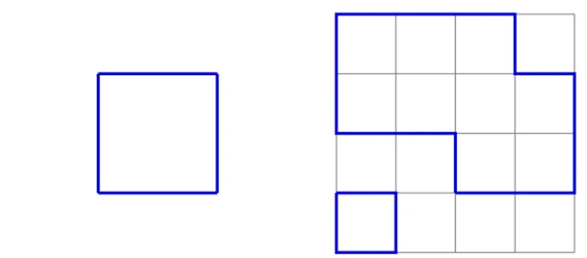
a vector changes when it is transported along an infinitesimal loop, so it is natural to build the action looking at the Wilson loops on the plaquettes, which are the elementary loops on a lattice. A plaquette, denoted as ⇤, can be identified with a sequence of four links
(x, µ) ! (x + aˆµ, ⌫) ! (x + aˆµ + aˆ⌫, µ) ! (x + aˆ⌫, ⌫) . Then, the corresponding Wilson loop is given by the following equation
tr W⇤ =tr⇥Uµ(x)U⌫(x + aˆµ)Uµ(x + aˆ⌫)†U⌫(x)†
⇤
. (1.39)
To compare it with continuum objects, we have to reintroduce the gauge potential Aµ(x). On an elementary path, the integral reduces to a
multipli-cation by the spacing a. Therefore, we can identify
Uµ(x) = eiaAµ(x). (1.40)
Substituting it into tr W⇤, one finds [32] that up to higher order terms
tr W⇤ =tr h eia2Fµ⌫(x)+ . . . i =tr I + ia2F µ⌫ a2 2Fµ⌫Fµ⌫+ . . . , where the indices µ, ⌫ are not summed on. Fµ⌫ is traceless and, working in
the fundamental representation of SU(N), tr I = N. Then it holds tr W⇤ = N + a
2
2tr Fµ⌫Fµ⌫+ O(a
1.4. Gauge fields on a lattice 23 Notice that, since FijFij = (Pk✏ijkBk)2and F0iF0i= Ei2, when the plaquette
⇤ sits on two space directions i, j tr W⇤ contributes to the magnetic term,
while the electric term is given by plaquettes along a space direction i and the time direction 0. To get rid of the constant term we can use tr(I W⇤)
instead. Then, we get an action that reduces to the continuum one in the limit a ! 0 if we sum on all plaquettes
SW[{Uµ(x)}] = 2 g2a4 D X ⇤ Re tr I W⇤ , (1.42)
where Re has been added because the sub-leading order terms may not be real. This is the Wilson action and it is the simplest gauge-invariant lattice action for gauge fields one can write; other possibilities exist, but they differ only in higher order terms. An explicit labeling for W⇤ is Wµ⌫(x), where x
is the origin of the plaquette and µ 6= ⌫ are the directions that identify the plane where it lies. Then, the sum on all plaquettes can be rewritten as a sum on all lattice sites x 2 ⇤ and on all directions 1 µ < ⌫ D, so that
SW = 2 g2a4 D X x2⇤ X µ<⌫ a4 2 tr Fµ⌫Fµ⌫ = aD 2g2 X x2⇤ X µ,⌫ tr Fµ⌫Fµ⌫,
where a factor 1/2 comes from the antisymmetry of Fµ⌫. We have proved
that the continuum limit is correct. An equivalent form of the action is SW[{Uµ(x)}] = 1 g2a D X ⇤ ⇣ tr W⇤+tr W⇤† ⌘ , (1.43)
because the constant term is non-dynamical and it can be neglected. The lattice path integral for gauge fields is defined in the following way:
Z = Z DU e SW[U ]⌘Z ⇣ Y (x,µ) dUµ(x) ⌘ e SW[{Uµ(x)}]. (1.44)
Each integral with differential dUµ(x) is done on the group manifold. The
proper integration measure that defines them is the Haar measure [58]. Its main property is that it is both left and right invariant: given a function f (U ) on the group SU(N), 8g 2 SU(N) it holds that
Z SU (N ) dU f (g· U) = Z SU (N ) dU f (U ) = Z SU (N ) dU f (U · g) , (1.45) meaning that the integral respects the gauge symmetry. Given an observable O, one is typically interested in computing the average
hOi = 1
Z Z
A gauge transformation maps the right hand side of this equation to Z
DU O({g(x + aˆµ)Uµ(x)g(x)†})e SW[{g(x+aˆµ)Uµ(x)g(x) †}]
,
which is equal to the original integral thanks to left and right invariance. But the action is gauge-invariant, so it also equals
Z
DU O({g(x + aˆµ)Uµ(x)g(x)†}) e SW[{Uµ(x)}]
for arbitrary functions g(x), implying that the average of a local observable hOi can be different from zero only when O is gauge-invariant. The special importance of Wilson loops is underlined by the following fact: any gauge-invariant observable that depends continuously on the link variables can be approximated arbitrarily well by polynomials of the kind [58]
1 X n=0 X 1... 2 a( 1, . . . , 2)tr W [ 1] . . .tr W [ n] . (1.47)
Another consequence of this fact is the important statement known as Elitzur’s theorem: gauge symmetries cannot be spontaneously broken [46].1
If a system has a symmetry, the order parameter that signal its spontaneous breaking has to be non-invariant under the symmetry transformation. But this fact implies that their expectation value will always vanish, so an SSB cannot happen. We have considered here only a quantum statistical system at zero temperature, the fluctuations are only quantum, but if we added also thermal fluctuations the results would be the same.
Consider for instance a “gauged” version of the Ising model, that has been modified to promote its Z2 global symmetry to a local one. Its gauge
symmetry cannot be broken, but nevertheless the phase diagram of this is non-trivial and it is an interesting issue to find an order parameter able to detect its transition. The key point is that we had assumed that O was a local function: on a gauge system phase transitions signaled by non-local order parameters can still happen.
1.5 Hamiltonian Yang-Mills theory
Path integrals are the standard tool used to study lattice gauge theories. However, the hamiltonian approach has some important advantages: truly
1It is often said that the Higgs mechanism corresponds to the SSB of a gauge symmetry.
This is misleading, as it is forbidden by Elitzur’s theorem: what is broken is only the global part of a local symmetry, while the redundancy still persists [28].
1.5. Hamiltonian Yang-Mills theory 25 dynamical phenomena can be described only in a real-time hamiltonian set-ting, which avoids also the sign problem when a chemical potential is added [8], has we have already discussed in the introduction. Moreover, the in-terpretations of the variables is more transparent, since the observables are treated as the usual operators on a Hilbert space. Before formulating the lattice theory in its hamiltonian version, let us quickly review the continuum case. Matter does not need additional considerations with respect to the free case, so we shall consider only the gauge part.
The main issue we have to deal with is gauge invariance: the lagrangian is written with some redundant non-dynamical degrees of freedom. This is reflected into the fact that LY M does not contain ˙A0
⇧0 = @LY M
@ ˙A0 = 0 ,
A0 is not dynamical, since it has no conjugate momentum. Then we can
isolate the A0 dependent part of LY M, thus finding [49]
LY M = 1 g2 tr ⇣ ~ E2 B~2⌘+ 1 g3 tr A0G (1.48) Ga(x) = Ea i(x) + fabcAbi(x)Eic(x) = DiEia(x) (1.49) again with G = GaT
a. A0 is a Lagrange multiplier and its equation of motion
corresponds to the phase space constraint DiEia(x) = 0: gauge theories are
constrained systems. DiEia(x) = 0is the generalization of the Gauss’s law:
when G is abelian, like for G=U(1), [Ai, Ei] = 0 and
DiEi(x) = ~r · ~E(x) = 0 .
Instead, non-abelian gauge fields, carry a colour charge and a density term is added. The quantization can be simplified by imposing a gauge fixing condition from the start. We work in the temporal gauge A0 = 0, in order to
quantize only the dynamical degrees of freedom Ai. Now, the lagrangian is
LY M = 1 g2tr ~E 2 B~2 = 1 2g2 E i aEai BaiBai and using Ei
a= A˙ia = ˙Aai we find the momentum conjugate to Aai
⇧ia= @LY M @ ˙Aa i = E i a g2 . (1.50)
The hamiltonian can be found from the Legendre transformation HY M = ⇧iaA˙ai LY M = 1 2g2 E i aEai + BaiBai (1.51) HY M = Z dDx HY M = Z dDx ✓ g2 2 ⇧ i a⇧ia+ 1 2g2B i aBai ◆ . (1.52)
To quantize the theory, we have to promote the fields to operators that satisfy canonical equal-time commutation relations
[ ˆAai(x), ˆAbj(y)]x0=y0 = 0 = [ ˆ⇧ia(x), ˆ⇧jb(y)]x0=y0 (1.53)
[ ˆAai(x), ˆ⇧jb(y)] = i ba ij 3(~x ~y) . (1.54) The simplest representation of these relations is probably achieved on the space of wavefunctionals h ~A(x) | i = [ ~A ]. Similarly to what happens in finite-dimensional quantum systems with [ˆxi, ˆpj] = i ij, Aai(x)acts on [ ~A ]
multiplicatively while ˆ⇧i
a is the generator of translations
ˆ Aai(x) [ ~A ] = Aai(x) [ ~A ] (1.55) ˆ ⇧ia(x) [ ~A ] = i Aa i(x) [ ~A ] . (1.56)
However, the Hilbert space of all wavefunctionals [ ~A ]is still too large. The temporal gauge keeps a residual gauge invariance for time independent gauge transformations A0 7! gA0g 1+ ig@0g 1, which is still vanishing if A0 = 0
and @0g = 0. At the quantum level, it means that
[ ~A ]⇠ [g ~Ag 1+ ig ~rg 1] , (1.57)
the two wavefunctionals should identify the same physical state. Classically DiEi(t, ~x) = 0, it is an integral of motion and it is promoted to a local
operator ˆG(~x) = DiEˆi(~x) (depending only on the spatial position, in the
Schrödinger picture) that commutes with the hamiltonian
[ ˆHY M, ˆG(~x)] = 0 . (1.58)
It can be shown that ˆG(~x) = DiEˆi(~x) is the quantum generator of
time-independent gauge transformations [27]. For instance, in the simpler abelian case the commutation relations (1.54) imply
ˆ R[ ] = exp ⇢ i g2 Z d3x (x)~r ·E(~x)~ˆ (1.59) ˆ R†[ ] ˆAj(~x) ˆR[ ] = ˆAj(~x) + @jˆ(~x) . (1.60)
If we apply the quantum version of the Gauss’s law constraint on the Hilbert space ˆG| i = DiEˆi(~x)| i = 0, the states that satisfy it are unchanged by
(1.60), so it is equivalent to (1.57) and applying it removes the residual gauge redundancy. In conclusion, we can identify the physical Hilbert space with
Hphys =
n
1.6. The Kogut-Susskind hamiltonian 27 If we included charged matter fields, the constraint term would be modified by including matter density. For instance, in QED the traditional Gauss’s law would be recovered as (~r ·E~ˆ q ˆ† )ˆ |physi = 0.
1.6 The Kogut-Susskind hamiltonian
The main difference between the path integral and the hamiltonian formalism for lattice theories is that for the hamiltonian one time can be kept real and continuous, while path integrals are formulated on a full spacetime lattice (with imaginary time). The hamiltonian should be the generator of time translations for all values of t on the real line. Two approaches can be followed to find the lattice hamiltonian.
One common approach to find the lattice hamiltonian is to use the transfer matrix formalism [46]. The idea is that for any lattice theory with discrete time, using the transfer matrix T⌧0,⌧, the partition function can be written as
Z =
N
X
n=0
h (⌧n+1, ~x)| ˆT| (⌧n, ~x)i = tr ˆTN, (1.62)
as long as there are periodic boundary conditions on the time direction. Taking advantage of the fact that the euclidean action represents the energy of the system, we can interpret the transfer matrix can as the generator of an imaginary time evolution between the two time slices ⌧n and ⌧n+1. The
duration of this time evolution equals the lattice spacing a, so that ˆ
T = e a[Hˆa+O(a)] . (1.63)
This defines the lattice hamiltonian, which is not a actual hamiltonian be-cause of the discrete time. However, if we place the theory on an inhomoge-neous lattice, with time spacing a0 kept different from the spatial spacing a,
we can perform the limit a0 ! 0, which recovers a continuous time. Then
ˆ
H = lim
a0!0
ˆ
Ha0. (1.64)
For point-like quantum system, whose path integral is defined only on a discrete time since they do not have a spatial extension, this limit recovers the correct quantum hamiltonian. Therefore this is a sensible definition also for field theories on a spatial lattice.
Instead of taking this route, we place directly a spatial lattice on the hamiltonian formulation of the continuum theory [57]. To recover the hamil-tonian (1.52), we recognize that the chromoelectric term and the chromomag-netic are the same appearing in the lagrangian but with the opposite relative
sign: the former behaves as a kinetic term, while the latter as a potential one. We already know how to discretize the lagrangian. The magnetic part of the Wilson action is given by a sum on all spatial plaquettes of tr W⇤ and this
can be repeated straightforwardly for the hamiltonian. Instead, some prob-lems appear for the electric term, which was obtained by summing tr W⇤ on
time-like plaquettes. Now the lattice is only spatial and time-like plaquettes do not exist anymore! We are not only unable to get the electric term like before, but also we cannot specify a group element Uµ(x) for µ = 0, since
there are no links in the time direction.
To avoid this issue, we perform again the quantization in the temporal gauge A0 = 0, so that time-like links become associated with the identity and
they do not affect comparators anymore [73]. Then, a classical configuration of the lattice pure-gauge theory is identified by the choice of a matrix U 2 SU(N) for all spatial links at a fixed time. The system can be seen as a many-body model made of several links, each one with SU(N) as its configuration space. Correspondingly, the Hilbert space of a single link can be identified with the wavefunctions : SU(N) ! C, with the usual requirement of being square integrable. The full Hilbert space is given by the tensor product
HNL = NL
O
`=1
L2 SU(N) = SU(N) ⌦ · · · ⌦ SU(N)
| {z }
links
. (1.65)
The wavefunctions (U) take as input the group elements, which define the analog of the position basis. We can promote the “position” of a single link U 2 SU(N) to a state |Ui 2 H1. The set { |Ui | 8U 2 SU(N)} is a
generalized basis of H1 = L2(SU(N)) satisfying the orthonormality relation
hU|V i = (U, V ), similarly to what happens with L2(R) and |xi [57]. The
physical (normalized) states will then be | i =
Z
dU (U )|Ui , 2 L2(SU(N)) (1.66)
where, as usual, dU represents the Haar measure on the gauge group. The single link Hilbert space we have just described is called by mathematicians the group algebra of SU(N); more details about it can be found in Appendix A. |Ui is an eigenstate of the “position” operators ˆUij
ˆ
Uij|Ui = |Ui Uij, (1.67)
associating to the link in the eigenstate |Ui the corresponding matrix ele-ments in the appropriate representation. Notice that ˆUij is neither
1.6. The Kogut-Susskind hamiltonian 29 the conjugate of (1.67) is hU|( ˆUij)†= Uij⇤hU|, which implies
hU| ( ˆUij)†Uˆij|Ui = Uij⇤UijhU|Ui 6= hU|Ui .
The adjoint “position” ( ˆUij)† acts also on kets as ( ˆUij)†|Ui = |Ui Uij⇤, since
for all bras h | =R dV (V )⇤hV | it holds that
h |⇣( ˆUij)†|Ui ⌘ ⌘⇣h |( ˆUij)† ⌘ |Ui = Z dV (V )⇤Vij⇤hV |Ui = (U)⇤Uij⇤ =) h |⇣( ˆUij)†|Ui ⌘ = h |Ui Uij⇤ 8 h | .
What prevents ˆUij from being unitary is that this conjugation does not
re-verse the order of the indices i, j . We can define the matrix of operators ˆU whose elements are ˆUij s.t. [ ˆU ]ij|Ui = |Ui Uij. Being a matrix, its hermitian
conjugate includes both a transposition and a Hilbert space adjunction
[ ˆU†]ij = ( ˆUji)†. (1.68)
When the chosen representation is unitary, the previous equation implies
hU|X j [ ˆU†]ijUˆjk|Ui = X j Uij⇤,tUjkhU|Ui = hU|Ui ,
meaning that the matrix of operators ˆU is the unitary object. At this point, we can define comparators on a path as Hilbert space operators [57]. Con-sider an elementary path e on a link ` and call ˆU [e] the comparator on it. Comparators are matrices in the colour space which map charged fields on the origin of the path into charged fields on the endpoint of the path. Like we did in the path integral case, we identify the group element on the link ` with the comparator ˆU [e]when the directions of e and ` coincide, otherwise they are the inverse of each other. So we have
ˆ U [e] = ( ˆ U (`) if e k ` ˆ U†(`) if e k ` , (1.69)
denoting with ` the link where the “position” matrix is placed. The com-parator on a general path = e1· ... · en, sequence of the elementary paths
e1, ..., en, is given by the composition
ˆ
U [ ] = ˆU [e1]· ... · ˆU [en] . (1.70)
If the path is closed, we can define the Wilson loop operator tr ˆW [ ] = tr⇣U [eˆ 1]· ... · ˆU [en]
⌘
For instance, when is a plaquette the previous equation yields
tr ˆW⇤ =tr ˆU (x, i) ˆU (x + aˆi, j) ˆU (x + aˆj, i)†U (x, j)ˆ † (1.72) We recover the magnetic part ˆHB by summing on all spatial plaquettes
ˆ HB = 1 g2a4 d X ⇤ ⇣ tr ˆW⇤+tr ˆW⇤†⌘. (1.73) The trace is giving the missing 1/2 factor with respect to (1.52), while the power of a is now d = D 1 because the lattice is only spatial.
To find the electric term, recall that in the continuum hamiltonian it is given by the square of ˆ⇧i
a = i / Aai, which generates translations on [ ~A ].
On a lattice we do not work with the potential ~A anymore and states are elements of the group algebra, i.e. square integrable functions SU(N) ! C, however, we can still write the electric term using the generator of trans-lations. Translations on the group algebra are defined through the regular representation (cf. Appendix A) of the gauge group: U acts on |V i as
ˆ
LU|V i = |UV i . (1.74)
The corresponding action of U on the wavefunction (V ) is given by ˆ
LU (V ) = (U 1V ). (1.75)
ˆ
Lis an infinite-dimensional unitary representations of SU(N) onto the space of wavefunctions L2(SU(N)) and it satisfies the relations
ˆ
L†ULˆU =I , ˆL†U = ˆLU†. (1.76)
Actually, this is only the left regular representation. One may also choose to work with the right regular representation ˆRU|V i = |V U 1i , which has
analogous properties and would lead to the same results. The momentum operator is proportional to the generator of translations, therefore we need to find the Lie algebra representation ˆ` of su(N) that corresponds to ˆL [71],
ˆ
` : su(N) ! End L2(SU(N)) .
Making use of the Lie exponential map, we can write any U 2 SU(N) as U = eiX, X 2 su(N). The compatibility of ˆ` and ˆL is encoded into
ˆ
1.6. The Kogut-Susskind hamiltonian 31 Expanding on the Lie algebra generators X = XaT
a, ˆLeiXaTa = ei X a`ˆa
. Here ˆ
`a ⌘ ˆ`(Ta) is the generator of su(N) in the regular representation, which is
the momentum operator we need. Being a representation, it satisfies
[ˆ`a, ˆ`b] = i fabc`ˆc. (1.77)
Notice that ˆ`a has only the Lie algebra index a, while the continuum
mo-mentum ˆ⇧i
a has also a spatial index i. The spatial direction is implicit on a
lattice, because ˆ`a is placed on a link (x, i), which is already characterized
by a specific direction i. The electric term, then, can be identified as ˆ HE = g2 2ad 2 X (x,i) X a ˆ `a(x, i)2. (1.78)
It contains the sum on all directions a of the squared generators of transla-tions, giving a generalization of the laplacian operator on the gauge group, while the external sum is over all spatial links (x, i). ˆ`a is a good choice for
the momentum operator because it has the correct continuum limit, implying that also ˆHE is the right electric term of the hamiltonian. This follows from
the lattice version of the canonical commutation relations [52]
[ˆ`a, ˆUij] = (TaU )ˆ ij (1.79)
[ˆ`a, ˆUij†] = ( ˆU†Ta)ij. (1.80)
To derive them, consider the one-parameter subgroup h(s) = eisXa. Under
the regular representation, [ˆLh(s) ](U ) = [eisˆ`a ](U ) = (e isXaU ).
Apply-ing a derivative and evaluatApply-ing it at s = 0, we find [ˆ`a ](U ) = i d ds ⇣ e isXaU⌘ s=0 , (1.81)
which is equivalent to ˆ`a = idsdLˆeisXa
s=0. One should apply this result
to the straightforward equality [ˆLU, ˆUij]|V i = (Vij (U V )ij) ˆLU|V i, taking
U = h(s). This allows to prove (1.79) and the second one can be found similarly. (1.79) implies that the action of ˆ`a on (U) can be represented as
ˆ
`a= (TaU )ij
@ @Uij
. (1.82)
After having reintroduced the potential U = eiaAaT
a, it can be shown [52] that
meaning that ˆ`ais the correct lattice expression for the momentum operator.
Putting together the two parts gives us the Kogut-Susskind hamiltonian ˆ HKS = g2 2ad 2 X (x,i) X a ˆ `a(x, i)2 1 g2a4 d X ⇤ ⇣ tr ˆW⇤+tr ˆW⇤†⌘ (1.83) which has to be though as the hamiltonian corresponding to the Wilson action in the temporal gauge [47]. Again, the A0 = 0 condition leaves a residual
freedom for time-independent gauge transformations. Gauge transformations act on the states of the system, that are now elements of a Hilbert space. On a single link (x, i), a gauge transformation is
|U(x, i)i 7! |g(x + aˆi) U(x, i) g(x)†i . (1.84) If we call a link e ⌘ (x, i), e = x the source site and e+ = x + aˆithe target
site, then the transformation is realized by the operator ˆJe: He ! He s.t.
ˆ
Je|U(e)i = |g(e+) U (e) g(e )†i = ˆLg(e+)Rˆg(e )|U(e)i . (1.85)
Overall, H =NeHe and the states are generated by the basis
N
e |U(e)i .
Since each factor of a tensor product of operators acts on its original space, the complete gauge transformation on the whole lattice is
ˆ
J: H! H , ˆJ=O
e
ˆ
Lg(e+)Rˆg(e ). (1.86)
One can check immediately that [ ˆHB, ˆJ] = 0 with a direct calculation. It
is less obvious that [ ˆHE, ˆJ] = 0, but it also holds. The reason is that the
electric term of each single link is proportional to the quadratic Casimir of the gauge group (see Appendix A), which acts trivially on each irreducible representation and the action of a gauge transformation is just a reshuffling of the states within the same representation. Together they yield
[ ˆHKS, ˆJ] = 0 (1.87)
and the Kogut-Susskind hamiltonian is gauge-invariant. The physical states will be selected by a Gauss’s law, requiring their gauge invariance
⇣ O e ˆ Lg(e+)Rˆg(e ) ⌘ |physi = |physi . (1.88)
1.7. Phase structure of gauge theories 33
1.7 Phase structure of gauge theories
The interest in lattice gauge theories was raised by Wilson, who showed that lattice QCD exhibits confinement in the strong coupling phase [90]. In gen-eral, both continuum and lattice gauge theories provide interesting phase diagrams, whose behaviour is often driven by complex non-perturbative ef-fects [66]. Notice that in the previous sections we have discussed only QFT at zero temperature. The lattice models we are considering have only quan-tum fluctuations and the transitions at T = 0 we encounter are quanquan-tum phase transitions. In order to outline a phase diagram, one usually studies some kind of order parameter. But remember the Elitzur’s theorem: gauge symmetries cannot undergo a spontaneous symmetry breaking and the usual local order parameters are insensitive to their phase transitions.
Only gauge-invariant objects can have non-vanishing expectation values, so a plausible candidate for the order parameter can be the Wilson loop. Indeed, they are be able to show a phase transition thanks to their non-local nature, which allows them to feel changes in global properties of the system, such as the emergence of topological excitations and topological phase tran-sitions [29]. However, other non-local order parameters do exist, such as the electric strings that will be described in the fourth chapter, or the ’t Hooft loops that were introduced to characterize SU(N) theories exploiting their Zn center symmetry [33, 38].
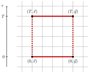
Let CR,T be the closed rectangular path consisting of the links
CR,T = (0, ~x; 0, ~y)· (0, ~y; T, ~y) · (T, ~y; T, ~x) · (T, ~x; 0, ~x) ,
where R = |~x ~y|, that is represented represented in Fig. 1.1. Let tr W [CR,T]
be the Wilson loop along it and consider its expectation value e.g. in the path integral formalism. Then
h tr W [CR,T]i = 1 Z Z DA tr W [CR,T] e SW ⇠ T!1 e V (R)T . (1.89)
V (R) is the so-called static quark potential and it represents the energy of a quark-antiquark pair which are kept fixed at a distance R [73].
A strong coupling expansion [32] allows to show that in lattice QCD V (R) ⇠ R when g ! 1 (and R is sufficiently large): the interaction be-tween the two quarks is like a spring which keeps them tied. When the distance between the quark-antiquark pair is increased, the energy grows until it overcomes twice the mass of the quark and it becomes energeti-cally favourable to break in halves the string and to produce another quark-antiquark pair. The two quarks cannot be separated, since, instead, we end
(0, ~x) (0, ~y)
(T, ~x) (T, ~y)
⌧
0 T
Figure 1.1: The loop CR,T on a spacetime lattice. It represents the
bound-ary of the worldsheet covered by the trajectory of a quark-antiquark pair fixed at positions ~x, ~y linked by a string of the gauge field.
up with two quark-antiquark pairs. This dynamical process is called string breaking mechanism and it characterizes the confined phase. In this limit, Wilson loops satisfy the area law
h tr W [CRT]i ⇠ e RT = e A[CR,T], (1.90)
where A[CR,T] is the area enclosed by CR,T. In the small coupling limit,
instead, V (R) ⇠ 1/R, yielding a Coulomb potential. This is easy to see also in continuum QCD. Considering the rescaled potential ˜Aµ, ˜Faµ⌫ = @µA˜a⌫ +
@⌫A˜aµ+ gfabcA˜bµA˜c⌫: when g ! 0 it reduces to the QED field strength and it is
natural to expect an electric-like interaction. This is the so-called Coulomb phase and it is deconfined, since we need a finite amount of energy to keet the two quarks infinitely distant. Of course, when R is large V (R) ⇠ 1/R does not contribute to the exponential damping of the Wilson loop. Other terms dominate and what holds now is the perimeter law [58]
h tr W [CRT]i ⇠ e ↵ p[CR,T], (1.91)
where now p[CR,T] indicates the perimeter of the loops CR,T. Another
com-mon possibility is a Higgs phase. It is still deconfined, but gauge fields develop a mass gap and Coulomb-like interactions undergo a screening, thus becoming short-ranged. Wilson loops in the Higgs phase satisfy again the perimeter law [28].
1.7. Phase structure of gauge theories 35 The proportionality constant is different from 0 if there is confine-ment, while it vanishes in decofined phases. Then, the string tension can be seen as an order parameter for the confinement-deconfinement transi-tion. To see why (1.89) holds, let us switch to the hamiltonian formalism. Here, working in the temporal gauge, the Wilson loop operator tr ˆW [CR,T] =
tr ˆU [0, ~x; 0, ~y] ˆU [0, ~y; T, ~y] ˆU [T, ~y; T, ~x] ˆU [T, ~x; 0, ~x] becomes
tr ˆW [CR,T] =tr ˆU [0, ~x; 0, ~y] ˆU [T, ~y; T, ~x] . (1.92)
Now consider a system with ˆH = ˆp2/2m + V (ˆx)in a euclidean time t = iT .
Then, its propagator is given by
K(T, x0; 0, x) =hx0|e HTˆ |xi !
m!1 (x x
0)e iV (x x0)T
. (1.93)
If the initial and final states are not eigenstates of the hamiltonian in the static limit m ! 1, we can expand them on the eigenstates |ni and
K(T, 0; 0, ) = X
n
h 0|nihn| i e EnT ⇠ T!1h
0|0ih0| i e E0T . (1.94)
The static limit can be taken again, thus leaving only the potential part of the energy. Now we repeat this procedure for the lattice theory. Consider a static quark-antiquark pair as the initial state
| 0i = ¯ˆ (0,~x) ˆU[0,~x; 0, ~y] ˆ (0, ~y) |0i . (1.95)
We had to include a Wilson line ˆU, connecting the two points (0, ~x) and (0, ~y), to make | 0i a gauge-invariant state: physically this means that two quarks
are always connected by a flux line of the gauge field. Their propagator is G(T, ~x0, ~y0; 0, ~x, ~y) =h0| T⇥ ¯ˆ (T, ~y0) ˆU [T, ~y0; T, ~x0] ˆ (T, ~x0)
¯ˆ (0,~x) ˆU[0,~x; 0, ~y] ˆ (0, ~y)⇤ |0i (1.96) In the same limits that we have considered above, this reduces to
G(T, ~x0, ~y0; 0, ~x, ~y) ⇠
m!1 T!1
3(~x0 ~x) 3(~y0 ~y) C(~x, ~y) e V (R)T . (1.97)
V (R) is the static quark potential and it is the lowest energy contained into the quark-antiquark state whose overlap with the ground is non vanishing. C(~x, ~y) is a function describing this overlap. But the two probes are static and the energy V (R) is only that of the gauge field, apart from self-energy terms. The static quarks can be decoupled from the dynamics and what
(1.96) does is essentially to compute (1.89), up to the trace which does not change the exponential damping.
This sketched proof holds for time-like Wilson loops, but the confinement criterion is correct also for Wilson loop that live on a fixed-time surface [86]. The reason is that a Wilson loop operator on a spatial closed path C can be seen as the creator of a loop of electric flux along C . Then h0|tr ˆW [C ]|0i becomes the tunneling amplitude of the electric flux loop into the vacuum, which is highly suppressed in the confined phase because flux tubes are sta-ble. Confinement is a property of the gauge field themselves and the tran-sition is driven by a drastic change in the properties of their vacuum. In fact, it is typically seen as a condensation of magnetic monopoles, which is somehow dual to the Cooper pair condensation of superconductors [22]. For instance, consider a U(1) pure-gauge theory. Polyakov showed that in three dimensions it is always in a confined phase thanks to the contribution of the instantons, forming a gas of magnetic monopoles which produces the linearly confining force between quarks. Thankfully, in four dimensions it has also a familiar small coupling Coulomb phase, in addition to the strong coupling confined phase [67, 68], while in 1+1 dimensions is trivially confining, since the Coulomb potential is already V (R) ⇠ R.
In general, it has been proven that for all compact gauge groups, both continuous and discrete, the corresponding LGT in any spacetime dimension has a confined phase for sufficiently strong couplings [58]. The behaviour of pure U(1) LGTs traces the continuum one: in D = 3 it is always confined, while in D = 4 there is also the Coulomb phase. The group U(1) can be approximated by Zn. In D = 3, a Zn LGT of course has a strong coupling
confined phase, but at small couplings it exhibits a deconfined Higgs phase (that can exist also in the pure gauge case, provided that it is defined accord-ing to the behaviour of Wilson and ’t Hooft loops [60, 26]), which shrinks and tends to disappear in the n ! 1 limit. When D = 4 the structure with a shrinking Higgs phase is similar, but the Coulomb phase appears only for Zn 5. We underline that the spatial Wilson loop criterion holds only at
zero temperature: discrete group LGTs at a finite temperature have an addi-tional deconfined phase with area law behaviour [12, 13]. For the SU(2) and SU(3) groups it is considerably harder to extract continuum analytical re-sults, while Monte Carlo lattice simulations using finite groups tend to show confinement at all couplings [20], even though QCD at small coupling has to be deconfined.
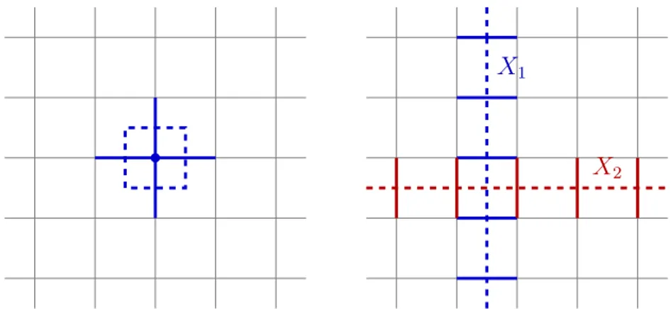
![Figure 4.3: The Wilson line operator W [C ] acts on the links where the path C lies, while the ’t Hooft loop operator X[ e C ] acts on the links crossed by the path on the dual lattice eC .](https://thumb-eu.123doks.com/thumbv2/123dokorg/7380619.96498/86.892.363.581.193.408/figure-wilson-operator-links-hooft-operator-crossed-lattice.webp)
![Gianluca D’Andrea, transito all’ombra, Marcos y Marcos, Milano, 2016. [Recensione]](data:image/gif;base64,R0lGODlhAQABAIAAAP///wAAACH5BAEAAAAALAAAAAABAAEAAAICRAEAOw==)