Comparative analysis of models and performance indicators for optimal service facility location

Transportation Research Part E 145 (2021) 102174

Available online 24 December 2020

1366-5545/© 2020 The Authors. Published by Elsevier Ltd. This is an open access article under the CC BY-NC-ND license (http://creativecommons.org/licenses/by-nc-nd/4.0/).

Comparative analysis of models and performance indicators for

optimal service facility location

Edoardo Fadda

a,c

_{, Daniele Manerba}

b

_{, Gianpiero Cabodi}

a

_{, Paolo Enrico Camurati}

a

_,

Roberto Tadei

a,

*

a_{Dept. of Control and Computer Engineering, Politecnico di Torino, 10129 Turin, Italy} b_{Dept. of Information Engineering, University of Brescia, 25123 Brescia, Italy}

c_{ICELAB: ICT for City Logistics and Enterprises Lab, Politecnico di Torino, 10129 Turin, Italy}

A R T I C L E I N F O

Keywords:

Facility location Key performance indicators Back-up coverage Progressive interventions

A B S T R A C T

This study investigates the optimal process for locating generic service facilities by applying and comparing several well-known basic models from the literature. At a strategic level, we empha-size that selecting the right location model to use could result in a problematic and possibly misleading task if not supported by appropriate quantitative analysis. For this reason, we propose a general methodological framework to analyze and compare the solutions provided by several models to obtain a comprehensive evaluation of the location decisions from several different perspectives. Therefore, a battery of key performance indicators (KPIs) has been developed and calculated for the different models’ solutions. Additional insights into the decision process have been obtained through a comparative analysis. The indicators involve topological, coverage, equity, robustness, dispersion, and accessibility aspects. Moreover, a specific part of the analysis is devoted to progressive location interventions over time and identifying core location decisions. Results on randomly generated instances, which simulate areas characterized by realistic geographical or demographic features, are reported to analyze the models’ behavior in different settings and demonstrate the methodology’s general applicability. Our experimental campaign shows that the p-median model behaves very well against the proposed KPIs. In contrast, the

maximal covering problem and some proposed back-up coverage models return very robust solutions

when the location plan is implemented through several progressive interventions over time.

1. Introduction

Facility location is a fundamental strategic aspect in the design of many processes, including logistical operations (e.g., hub

location) and specific transportation/routing applications (e.g., the location of charging stations for electric vehicles). Moreover, it is

widely applied in cases where some geographical areas must be covered in terms of commercial reachability (e.g., opening new shops

by a firm) or public and private services (e.g., the location of the metro stations or transmitting antennas). Therefore, facility location

problems have been studied since a long time (see

Miehle, 1958

or

Cooper, 1963

), and still attract considerable research attention (see,

e.g.,

Labb´e et al., 2019; Cherkesly et al., 2019; Brandst¨atter et al., 2020

, or

Lin et al., 2020

). In particular, as described in Section

2

, the

* Corresponding author at: corso Duca degli Abruzzi 24, 10129 Turin, Italy.

E-mail addresses: edoardo.fadda@polito.it (E. Fadda), daniele.manerba@unibs.it (D. Manerba), gianpiero.cabodi@polito.it (G. Cabodi), paolo. camurati@polito.it (P.E. Camurati), roberto.tadei@polito.it (R. Tadei).

Contents lists available at

ScienceDirect

Transportation Research Part E

journal homepage:

www.elsevier.com/locate/tre

https://doi.org/10.1016/j.tre.2020.102174

most recent literature focuses on particular and tailored models. Instead, in this work, we focus on fundamental and general location

models.

In the planning phase of a facility-location process, two main common decision scenarios may occur. In the first scenario, the

decision-maker is still evaluating higher-level plans. Therefore, it is interesting to know, for example, the minimum number of facilities

to locate or the minimum budget to allocate to achieve a certain level of service or coverage. In the second scenario, the decision-maker

has a pre-allocated budget for the facilities and their operations, implying an a priori knowledge of the exact number of facilities to

locate. In this study, we only focus on the latter scenario and leave the former for future studies. The decision to consider first the

situation in which the number of facilities to locate is an input for the problem is motivated by several reasons: a) it represents a more

practical operational setting, given a preliminary economic analysis of the investment; b) it can support the study of a decision process

divided into several planned interventions (see Section

4.4

); and c) it can support the analysis of the robustness of the solutions (back-

up coverage) against congestion or other external disruptions.

At a strategic level or during the exploratory phases of a decision process, selecting the right location model to use could result in a

problematic and possibly misleading task if not supported by appropriate quantitative analysis. In fact, in real settings, all the

re-quirements and factors to consider inside the optimization process are often not completely clear (due to externalities, uncertainty,

etc.). Several incomparable objectives should be taken into account (conflicting interests of different stakeholders). Finally, especially

in industrial applications (see, e.g.,

Fadda et al., 2018, 2019a; Giusti et al., 2019

), it is a good practice for the management to consider a

joint evaluation, through several performance indicators of interest, of the behavior of the solutions coming from different models. For

this reason, we propose a general methodological framework to analyze and compare the solutions provided by several models from

the literature to obtain a comprehensive evaluation of the location process from several different perspectives and thus to provide

decision-makers with insights on strategic location management. Different models address different objectives, but they can be

reasonably comparable in terms of solution features if the returned solution contains the same type of decisions, i.e., a subset of

fa-cilities to locate. Since a single model takes care of a single indicator (its objective function), we believe it is crucial to understand how

the returned solutions behave against several other indicators (even if the model does not explicitly consider them). Therefore, a

battery of key performance indicators (KPIs) has been developed and calculated for the different models’ solutions. The analyzed KPIs

include topological aspects, covering capabilities, robustness, and accessibility of the resulting solutions. Besides topological and

coverage measures, we mainly focus on back-up models (to address congestion issues implicitly) and equity measures. Moreover, as

some types of service infrastructures are commonly supposed to be located through several progressive interventions over a defined

time horizon, we also provide ad-hoc KPIs measuring the flexibility of the solutions regarding location changes and objectives changes

over time. Furthermore, performing a comparative analysis of several models allows us to provide additional insights for the decision

process itself via the study of the percentage of locations that always (or almost always) appear in the optimal solutions. Through this

analysis, the decision-maker can choose the favorite location model by looking at several features of the possible solutions provided

and not just by assuming that a particular specific indicator is the correct one to optimize.

It is essential to state that our perspective and thus our models and KPIs are related to the location of service facilities, i.e., those

facilities that the decision-maker prefers to locate, ideally, at the least possible distance from demand centers. Here, the best coverage

and accessibility of a service facility concerning the territory is pursued. Instead, our analysis is not directly applicable for obnoxious

facilities, i.e., those facilities that the users would like to have as far as possible (e.g., nuclear waste processing plants). However, we

remark that our general evaluation framework could consider tailored models and KPIs for obnoxious facilities.

The main research questions addressed in this paper are: (i) How to support the management in selecting the most appropriate

location model for the application at hand? (ii) Can we derive general managerial insights for service location processes without

considering strongly customized input data? To this aim, we (i) propose a general methodological framework to quantitatively analyze

and compare the solutions provided by different location models and (ii) experimentally validate such a method to provide managerial

insights for service facility location processes. These points represent the principal contributions of our study. The administrations can

use the analysis to decide how to locate their available facilities to optimize the quality of their service from several perspectives. It is

worth noting that this approach cannot be found in the location literature, despite it has proven to be valuable and appreciated by the

management and a useful tool in real applications. Moreover, several classes of proposed KPIs (e.g., equity, progressive interventions,

and core measures) may be seen as contributions themselves.

The general applicability of our analytical approach is proved through three types of datasets simulating realistic features (e.g.,

densely or poorly populated areas and regions with particular geographical features) to provide strategic insights for location planning.

Eventually, our experimental campaign will show that the p-median model results in very well concerning both topological and equity

aspects. In contrast, the p-center and the maximal covering problem outperform the other models in terms of coverage capabilities.

Finally, the maximal covering problem and some proposed back-up coverage models return very robust solutions when the location plan is

implemented through several progressive interventions over time. However, with an appropriate calibration of the framework

components (i.e., models, KPIs, and their importance), similar insights can be easily gathered by the management in any specific real

applications.

The remainder of this paper is organized as follows. In Section

2

, we review the recent scientific literature related to facility

location. Section

3

is devoted to presenting and discussing several well-known basic models from the literature with different features

and objectives. In Section

4

, we propose and discuss different topological, coverage, equity, progressive intervention, and core solution

indicators. In Section

5

, the experimental results obtained are analyzed in terms of possible insights into the decision process. Finally,

2. Literature review

Location theory is one of the most important and oldest branches of logistics, with more than a century of history (

Laporte et al.,

2015

). Therefore, the available solution methods and modern solvers can quickly solve large-sized classical location problems (p-

center, p-median, etc.). Furthermore, the importance of location choices, deeply influence lower-level decisions as routing (see

Korte

and Vygen, 2008 and Perboli et al., 2018

) and flow optimization (

Giusti et al., 2021

). Hence, in recent years, the researchers involved

in the field have mainly focused on the definition and solution of complex location problems inspired by real applications.

We can identify four principal branches of research: bilevel, capacitated, stochastic, and work-balance models. The most recent

bilevel models are described in

Dan and Marcotte (2019), Liu et al. (2019), Farahani et al. (2019), Arulselvan et al. (2019), Guo et al.

(2018), Wenxuan et al. (2019), Lin et al. (2019), Chen et al. (2020)

. All these papers define a bilevel problem in which the first level

considers the facilities’ location, and the second one considers the optimization of the flow. The solution methods proposed are

heuristics due to the problems’ combinatorial aspects and the models’ complexity. Multilevel models have been considered too (

Ortiz-

Astorquiza et al., 2019

). These models are more complex than the bi-level ones; thus, the solution method presented is usually

heu-ristic. The most recent papers considering capacitated models are

Irawan et al. (2019), Raghavan et al. (2019)

. They address real-sized

problems in logistics characterized by a network with capacitated arcs. As for bilevel programs, the authors develop heuristics to solve

the problems. In the stochastic branch, the models assume that the network is subject to stochastic variations in the flows once the

locations have been selected. Those variations are usually represented by a discretization of the probability distributions using

sce-narios. This choice requires a large number of new variables, which increases the complexity of the model. Therefore, to solve the

problem, the authors implement heuristics (

Yu and Zhang, 2018

). Finally, workload balance features have been studied within location

problems (see, e.g.,

Davoodi, 2019

). Once used only in telecommunications, this aspect is now gaining much interest because of its

smart cities’ applications. As in the other branches, the complexity of the problems considering workload balance requires the

defi-nition of ad-hoc heuristics to solve real-size instances.

All the works just described develop tailored models and techniques suitable for a particular application. For example, the most

trending applications of the location theory are related to charging stations for electric vehicles (

Cai et al., 2014; Shahraki et al., 2015

),

electrical batteries in an electric grid (

Bose et al., 2012

), and sensors in distributed networks (

Muradore et al., 2006

). It is important to

note that it is not easy to generalize solutions tailored to problems in a specific setting to other applications. Furthermore, decision-

makers often want to evaluate the optimization process’s solution in several real-life applications and projects. They do that often

through many features that are exogenous to the model itself (i.e., KPIs) and possibly related to political preferences or human factors

(see, e.g.,

Tadei et al., 2016; Fadda et al., 2016, 2017, 2018, 2019b; Giusti et al., 2019

). Therefore, in this study, we develop a

framework for comparing, under different perspectives, the solutions obtained by solving different location problems. In particular, we

focus on common location problems because they can be solved several times in a few seconds. It is important to note that the

framework developed is model-independent and can be used for other models. In a similar spirit,

Ertugrul and Karakasoglu (2008)

develop a fuzzy multi-criteria decision-making method to overcome the inadequacy of standard mathematical models for facility

location selection due to the imprecise or vague nature of linguistic assessment.

To our knowledge, a general methodological framework to quantitatively analyze and compare the solutions coming from different

models has never been proposed in the location literature. A few papers have explicitly compared location models on just some

particular aspects (like coverage capabilities or equity). However, their vision is quite limited and tailored for a specific application

only. For example, in

van den Berg et al. (2016)

, the authors compare four static ambulance location models according to coverage and

response time criteria, proving that two models perform exceptionally well overall the considered criteria. Instead,

Yu and Solvang

(2018)

compare the solutions provided by p-median and maximal covering problem for locating post offices. The results provide

optimal relocation plans concerning different scenarios. Besides, a comparison between the optimal strategy and the current relocation

plan is given. However, in this work, the authors cannot identify a strictly better model than the others. In

Karatas et al. (2016)

, the

authors propose a more general comparison between p-median and maximal coverage problems and assess their performance. They

concern five decision criteria under redundant coverage requirements, namely, mean distance to facility, mean distance to primary and

back-up, mean distance to back-up(s), the ratio of demand served by both primary and back-up coverage within a range threshold, and

the ratio of demand served by at least primary coverage within a range threshold. Their methodology involves generating multiple

scenarios and solving the two models under each scenario. The experimental results show that, in general, p-median outperforms

maximal coverage in four criteria out of five.

Tansel et al. (1983)

did a similar evaluation, where he compared the p-center and the p-

median solutions over instances for several different settings to find common network features of the solutions (this is similar to what

we are going to call the core solution in Section

4.5

). Their comparison is made by just comparing the results coming from 60 references

papers from 1978 on. Note that, even if the last two mentioned papers follow our work’s same philosophy, they lack a comprehensive,

flexible, and structured procedure for comparing many different models under many different perspectives.

We finally remark that the comparison of different available models (or solving techniques) thought suitable frameworks is a very

common practice out of the pure optimization literature, as in Data Analytics, Machine Learning (ML), Artificial Intelligence (AI),

Computer Science, and Network Theory ones (see, e.g.,

Cordier et al., 2004; Ghanbari et al., 2010; Kumar and Singh, 2018; Cuzzocrea

et al., 2019; Castrogiovanni et al., 2020

). Interesting enough, in the AI and ML fields, location problems have been considered from the

point of view of prediction (see, e.g.,

Anagnostopoulos et al., 2011 and Cho, 2015

) but, to our knowledge, there is no specific studies in

3. Mathematical models for optimal location

In this section, we propose and discuss several well-known basic location models from the literature. In our analysis, we have

decided to include models for which a mixed-integer linear programming (MILP) formulation is available to be able to optimally solve

relatively large cases in a reasonable amount of time by merely inputting the explicit models into some powerful MILP solvers available

(e.g., Cplex or Gurobi). We focus on two families of problems: basic location models (p-median, p-center, p-centdian, and maximal

covering problem) and back-up coverage models (BACOP1 and BACOP2). We do not consider ad-hoc models because we aim to measure

how effective the standard model solutions result in the general setting. Furthermore, we do not consider covering problems because

they do not allow enforcing the number of facilities to locate so to consider the decision-maker’s budget limit.

Throughout the study, we will use the following general notation (specific additional notation will be presented below as

neces-sary):

•

G = (N,E): complete undirected graph with a set of nodes N representing possible locations for the facilities and a set of edges E =

{(

i,j)|i,j ∈ N,i⩽j};

•

d

: distance between node i and node j ∈ N (for the sake of simplicity, we will assume that the triangular inequality holds for the

distances, that is, d

⩽

d

+

d

, ∀

i < j < q ∈ N);

•

h

:=

Q

/

∑

Q

: demand rate of node i ∈ N, where Q

is the service demand in node i;

•

p: predefined number of facilities to locate, with p⩽|N|;

•

d: coverage radius, that is, the threshold distance to define the covering (it could represent, for example, the maximum distance that

an electric vehicle can travel or that a user is willing to drive to reach a facility);

• 𝒞

= {

j ∈ N,d

⩽

d}: covering set of i ∈ N, that is, the set of all facilities closer than d to node i.

Please note that set E also contains self-loops (i, i) on each node i ∈ N, i.e., we do not assume that the internal distances are strictly

equal to 0. In several applications, for example, where nodes represent non-punctual areas such as districts inside a town, the internal

distances d

between a service center and the actual demand might be non-negligible.

3.1. Basic location models

The following models are called basic because they do not explicitly pursue any redundancy or robustness of the solution. Note that

all the formulations include the requirement to locate exactly p facilities. We define y

as a binary decision variable taking the value 1 if

a facility is located in node j ∈ N, and 0 otherwise.

3.1.1. p-median

The p-median problem is to find p nodes of the network where to locate the facilities minimizing the weighted average distance

between the located facilities and demand nodes. It can be stated as

min

∑

h

∑

d

x

(1)

subject to

∑

x

=

1

∀

i ∈ N

(2)

∑

y

=

p

(3)

∑

x

⩽|N|y

∀

j ∈ N

(4)

y

∈ {0, 1} ∀j ∈ N

(5)

x

∈ {0, 1} ∀(i, j) ∈ E

(6)

where x

is a binary variable for edge (i,j) ∈ E, which takes the value 1 if and only if the demand in node i ∈ N is served by a facility

located in j ∈ N. Minimizing the objective function

(1)

involves minimizing the average distance traveled by the total demand flow

toward the facilities. The constraints

(2)

ensure that each demand node is served by exactly one facility. The constraint

(3)

ensures that

exactly p facilities are located. The logical constraints

(4)

ensure that all facilities to which demand nodes are assigned need to be

located/built. Finally,

(5) and (6)

state binary conditions on the variables.

3.1.2. p-center

its closest facility. In the proposed version of the problem, sometimes called the vertex restricted p-center problem, the facilities can be

located only at the nodes of the graph. The problem is focused on the worst-case and can be stated as

minM

(7)

subject to

M⩾

∑

j∈N|(i,j)∈E

h

d

x

∀

i ∈ N

(8)

and the already presented constraints

(2)–(6)

. Minimizing the objective function

(7)

involves minimizing the auxiliary variable M,

which, according to the constraints

(8)

, takes the maximum value of the expression

∑

h

d

x

over all nodes i ∈ N.

3.1.3. p-centdian

In the p-centdian problem, we want to find p nodes where to locate facilities to minimize a linear combination of the objective

function of the p-median and p-center problems presented above. The formulation is then

minλM + (1 − λ)

∑

h

∑

d

x

(9)

subject to

M⩾

∑

h

d

x

∀

i ∈ N

(10)

and the constraints

(2)–(6)

. Through the parameter λ, with 0⩽λ⩽1, it is possible to define the relative importance of one objective with

respect to the other one.

3.1.4. Maximal covering problem

In the maximal covering problem (MCP), differently from the well-known set covering problem, there is a predefined number p of

facilities to locate to maximize the coverage (

Church and ReVelle, 1974

). It can be stated as

max

∑

h

w

(11)

subject to

∑

y

=

p

(12)

w

⩽

∑

y

∀

i ∈ N

(13)

y

,

w

∈ {0, 1} ∀i ∈ N

(14)

where w

is a binary variable taking the value 1 if node i is covered, and 0 otherwise. Maximizing the objective function

(11)

involves

maximizing the total demand covered by the located facilities. The constraint

(12)

ensures that exactly p facilities are located whereas

the constraints

(13)

represent the logical link between the w and y variables.

3.2. Back-up coverage models

Models explicitly pursuing coverage redundancy are useful for creating solutions robust to congestion at the facilities or other

unpredictable events like failures or temporary unavailability. Back-up coverage problems have been extensively treated in

Hogan and

ReVelle (1986)

and still attract attention concerning modern applications (see

Johnson et al., 2020

). In the following, two classical

back-up models (again requiring that exactly p facilities must be located) are considered.

3.2.1. BACOP1

The back-up coverage problem of type 1 (BACOP1) can be stated as

max

∑

h

u

(15)

subject to

∑

y

=

p

(16)

u

+

1⩽

∑

j∈𝒞i

y

∀

i ∈ N

(17)

y

,

u

∈ {0, 1} ∀i ∈ N

(18)

where u

is a binary variable taking the value 1 if demand node i is covered at least twice, and 0 otherwise. Maximizing the objective

function

(15)

involves maximizing the number of demand nodes that are covered twice by a facility. The constraint

(16)

ensures that

exactly p facilities are located whereas the constraints

(17)

ensure that u

=

0 when location i is not covered by at least two facilities in

𝒞

.

It is essential to notice that, in contrast to the other location models presented, the BACOP1 returns feasible solutions only if there

are at least enough facilities to cover all the demand nodes once. It is easy to see that the constraints

(17)

cannot be satisfied when their

right-hand sides are strictly less than 1.

3.2.2. BACOP2

The back-up coverage problem of type 2 (BACOP2) represents a trade-off between basic and back-up coverage. It can be stated as

max

α

∑

h

u

+ (1 −

α

)

∑

h

w

(19)

subject to

∑

y

=

p

(20)

u

⩽w

∀

i ∈ N

(21)

u

+

w

⩽

∑

y

∀

i ∈ N

(22)

y

,

w

,

u

∈ {0, 1} ∀i ∈ N

(23)

where w

is a binary variable taking the value 1 if demand node i is covered at least once, and 0 otherwise. Maximizing the objective

function

(19)

involves maximizing a linear combination of nodes covered once and twice, weighted by a parameter 0⩽

α

⩽1. The

constraints

(21)

ensure that if a node is covered at least two times, then it is also covered at least one. The constraints

(22)

ensure that

the sum u

+

w

cannot exceed the number of times that location i is covered by facilities in 𝒞

. This means that, when u

=

1 then also

w

=

1 and therefore the number of covering facilities must be greater or equal than two, while when w

=

1 the number of covering

facilities must be greater or equal than one. It is easy to see that, when

α

=

0, the BACOP2 reduces to the MCP.

We want to indicate that, originally, the BACOP2 emerged as a pure multi-objective problem. To maintain uniformity with the

other problems, we provide and solve a formulation in which the objective function has been linearized. This practice is common as per

literature (see, e.g.,

Aringhieri et al., 2007; Aringhieri et al., 2016; Kahraman and Topcu, 2017

). Moreover,

α

can be seen as a further

possible parameter controlled by the decision-maker, and therefore, we will obtain BACOP2 results for several values of

α

without

considering the extreme degenerate cases. We will call each version of the problem BACOP2-

α

, with

α

= {

0.01,0.25,0.50,0.75,0.99}.

4. KPIs

This section defines an extensive battery of KPIs, thus providing several different noteworthy measures of the goodness of a location

solution. The identified KPIs are intended to outline an overview of the advantages and drawbacks of the different possible solutions to

help managements decide which model would be the best to implement. We emphasize that our KPIs consider spatial measures

(dispersion, average distance, etc.) as well as coverage, equity, and accessibility indicators (which are particularly crucial for services

offered to communities) and solution robustness measures in future expansions of the facilities.

The considered KPIs have been selected by looking at the desired features that a decision-maker would like to find in a location

plan. In particular, we believe that a solution could be analyzed from a topological perspective and in terms of coverage qualities and

equity measures in services for communities. Whenever possible, we will study the worst, best, and average perspectives of a measure.

Moreover, the behavior of such solutions over time takes particular importance in long-term implementations. Finally, finding the core

solution raises several insights on the riskiness of the decision-making process itself.

Some conducted industrial projects support our choices (see, e.g.,

Fadda et al., 2019a

), in which a subset of those KPIs have been

presented and appreciated by the management. However, it is essential to remark that other KPIs can be considered for a specific case,

or non-interesting KPIs can be eliminated from the analysis. This means that the set of KPIs is a flexible dimension to calibrate to apply

our analysis.

The selected KPIs, which we divide in topological, coverage, equity, progressive intervention, and core solution indicators, are listed and

discussed in the following subsections. We will use the following additional notation:

• ℒ = {

j ∈ N | y

=

1}: set of nodes where a facility has been located;

• ℒ

= {

j ∈ 𝒞

|

y

=

1}: set of nodes where a facility that covers demand node i has been located;

• 𝒞 = {

i ∈ N

⃒

⃒

⃒ ∃

j ∈ 𝒞

:

y

=

1}: set of demand nodes covered by at least one facility.

4.1. Topological KPIs

We first present KPIs based on the solution’s topological aspects but not considering the facilities’ covering capability (i.e., they do

not depend on the coverage radius d). They mainly concern distance, dispersion, and accessibility aspects.

•

WORST-CASE DISTANCE

D

:=

max

i∈N

min

d

(24)

represents the maximum distance between a demand node and its closest facility. This indicator measures the longest distance that

a user of the service has to travel to reach the nearest facility.

•

WEIGHT OF THE WORST-CASE DISTANCE

D

max

:=

h

:

arg max

i∈N

min

d

(25)

represents the demand rate affected by the worst-case scenario in terms of distance.

•

BEST-CASE DISTANCE

D

:=

min

i∈N

min

d

(26)

represents the minimum distance between a demand node and its closest facility. This indicator measures the shortest distance that

a user of the service has to travel to reach the nearest facility.

•

WEIGHT OF THE BEST-CASE DISTANCE

D

min

:=

h

:

arg min

i∈N

min

j∈ℒ

d

(27)

represents the demand rate affected by the best-case scenario in terms of distance.

•

AVERAGE DISTANCE

D

:=

1

|

N|

∑

min

d

(28)

represents the average distance between a demand node and its closest facility. This indicator measures the average distance that a

user has to travel to reach a facility.

•

WEIGHTED AVERAGE DISTANCE

D

:=

1

|

N|

∑

min

h

d

(29)

represents the average distance, where each node is weighted by its demand rate.

•

DISPERSION

Disp :=

∑

∑

d

(30)

represents the sum of the distances between all the located facilities. It is a measure of the homogeneity of the service from a purely

geographical point of view.

•

ACCESSIBILITY

Acc :=

∑

i∈N

h

A

(31)

is the total accessibility of the service, where

A

:=

∑

j∈ℒ

e

(32)

is the accessibility of a facility in the sense of

Hansen (1959)

. Accessibility is a measure of each demand node’s visibility on the

represents the dispersion of the alternatives in the decision-making process. The calibration is performed according to

Tadei et al.

(2009)

and

Fadda et al. (2020)

. The parameter β can be seen as a distance deterrence factor for locating.

4.2. Coverage KPIs

Here, we present KPIs based on covering aspects of the solution, and therefore, depending on the coverage radius d. Coverage KPIs

are extremely important, since the very final aim of a location problem for service facilities is to make the service available to the

demand centers.

•

COVERAGE

C := 100

*|𝒞|/|N|

(33)

represents, as a percentage, the number of covered locations with respect to the total.

•

WEIGHTED COVERAGE

C

_:=

₁₀₀

_*

∑

h

(34)

represents, as a percentage, the demand rate of the covered locations with respect to the total demand (note that, by definition,

∑

i∈N

h

=

1).

•

WEIGHT OF THE REDUNDANT COVERAGE

RC

_:=

_100*

∑

∑

j∈ℒi

h

(35)

represents, as a percentage, the demand rate of the covered locations multiplied by the times these locations are covered. This

indicator measures the weighted redundancy of the coverage.

•

WORST-CASE COVERAGE

C

:=

min

i∈N

|ℒ

|

(36)

represents the minimum number of facilities covering a demand node. This indicator measures the availability of different choices

for the unluckiest user (worst-case scenario).

•

WEIGHT OF THE WORST-CASE COVERAGE

C

min

:=

h

:

arg min

i∈N

⃒

⃒

⃒

⃒ℒ

⃒

⃒

⃒

⃒

(37)

represents the demand rate affected by the worst-case scenario in terms of coverage.

•

BEST-CASE COVERAGE

C

:=

max

i∈N

|ℒ

|

(38)

represents the maximum number of facilities covering a demand node. This indicator measures the availability of different choices

for the luckiest user (best-case scenario).

•

WEIGHT OF THE BEST-CASE COVERAGE

C

max

:=

h

:

arg min

i∈N

⃒

⃒

⃒

⃒ℒ

⃒

⃒

⃒

⃒

(39)

represents the demand rate affected by the best-case scenario in terms of coverage.

•

AVERAGE COVERAGE

C

:=

1

|

N|

∑

|ℒ

|

(40)

represents the average number of facilities covering a demand node.

•

WEIGHTED AVERAGE COVERAGE

C

:=

1

|

N|

∑

h

|ℒ

|

(41)

4.3. Equity KPIs

Apart from topological and coverage aspects, in several applications, it is essential to consider equity indicators. When the located

facilities are public services managed by municipalities, equity is an exciting dimension to study. For a more detailed analysis of equity

considerations in location problems, we refer the reader to

Barbati and Piccolo (2016)

. In the following, we present some simple equity

KPIs concerning coverage, distance, and accessibility.

•

EQUITY OF COVERAGE

EC :=

max

i∈I

(|ℒ

|) −

min

(|ℒ

|)

max

i∈I

(|ℒ

|)

(42)

represents the relative difference between the most covered and the least covered demand node.

•

EQUITY OF WEIGHTED COVERAGE

EC

_:=

max

i∈I

(|ℒ

| /

h

) −

min

(|ℒ

| /

h

)

max

i∈I

(|ℒ

| /

h

)

(43)

is a weighted version of the EC indicator. Here, the cardinality of ℒ

is divided by the relative importance h

of a node to assign a

larger weight to nodes with a smaller proportion of the demand.

•

MEAN ABSOLUTE DISTANCE DEVIATION

D

:=

1

|

N|

∑

⃒

⃒

⃒

⃒min

d

−

D

⃒

⃒

⃒

⃒

(44)

represents the mean absolute deviation (MAD), in terms of distance, of the demand nodes with respect to the nearest located

fa-cility.

•

WEIGHTED MEAN ABSOLUTE DISTANCE DEVIATION

D

:=

∑

h

⃒

⃒

⃒

⃒min

d

−

D

⃒

⃒

⃒

⃒

(45)

where h

:= (

1 − h

)/(|

N| − 1) is the complementary importance of node i. It is a weighted version of the D

indicator. Notice that

we use these particular weighting factors to maintain their summation equal to 1, as for the h

. Indeed,

∑

h

=

1

|

N| − 1

∑

(1 − h

) =

1

|

N| − 1

(

|

N| −

∑

h

)

=

|

N| − 1

|

N| − 1

=

1.

•

MEAN ABSOLUTE ACCESSIBILITY DEVIATION

A

:=

1

|

N|

∑

|

A

−

Acc|

(46)

represents the MAD in terms of accessibility for a demand node with respect to all the located facilities.

•

WEIGHTED MEAN ABSOLUTE ACCESSIBILITY DEVIATION

A

mad

:=

∑

i∈N

h

|

A

−

Acc|

(47)

is a weighted version of the A

indicator.

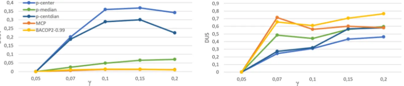
4.4. KPIs for progressive interventions

The decision-maker often does not have sufficient resources to install all the necessary facilities simultaneously; therefore,

installation plans are generally divided into several interventions programmed over time. Let S = {1, 2, …, 𝒮} be the set of installation

steps over the predefined time horizon and p

the number of facilities to locate at step s ∈ S. Clearly, in the case of progressive

in-terventions, in each step, we can only upgrade the solution already implemented in the previous inin-terventions, that is, previously

located facilities cannot be uninstalled. Therefore, it is crucial to understand (given a specific location model) how much the upgrading

solution of a specific intervention differs, in terms of objective function or structure, from the solution obtained under no conditioning

on previous decisions.

Since the simple calculation of the already presented KPIs at different installation steps is not sufficient to capture how the different

location models behave against an incremental expansion of the location plan, we propose the following ad-hoc KPIs to evaluate the

dynamic performance of a solution.

•

DEVIATION OF UPGRADED SOLUTION VALUE (at step s⩾2)

DUSV

:= |

f (p

) −

f (p

|

p

, ∀s

⩽s − 1)|

f (p

|

p

, ∀s

⩽s − 1)

(48)

measures the degree of influence of the previous choices in terms of the optimal objective function. In

(48)

, f(p

)

represents the

optimal objective function of the problem with parameter p = p

whereas f(p

|

p

, ∀

s

′

⩽

s − 1) represents the optimal objective

function of the problem with parameter p = p

, under the constraint that no facility can be removed from those located in the

solutions of all the problems with parameter p = p

,

s

′

⩽

s − 1. Because the KPI cannot be calculated for s = 1, we simply define

DUSV

:=

0.

•

DEVIATION OF UPGRADED SOLUTION (at step s⩾2)

DUS

:= 〈

y

(

p

),

y

(

p

|

p

, ∀s

′

⩽s − 1)〉

p

(49)

measures the degree of influence of the previous choices in terms of the optimal solution, where 〈v, v

〉

is the scalar product between

vector v and v

in R

_{. Similarly to above, in}

₍₄₉₎

_{, y}

₍

_p

s

)

represents the vector of the optimal solution of the problem with parameter

p = p

whereas y

(

p

|

p

, ∀

s

⩽

s − 1) represents the vector of the optimal solution of the problem with parameter p = p

, under the

constraint that no facility can be removed from those located in the solution of all the problems with parameter p = p

, ∀

s

′

⩽

s − 1.

Since the vector components are either 0 or 1, the scalar product is equal to the number of facilities that have been located in both

solutions. Again, because this KPI cannot be calculated for s = 1, we simply define DUS

:=

0.

It is worth noting that the decision-maker can choose how many steps it makes sense to consider (i.e., |S|) and the number of

facilities p

to locate in each step s ∈ S.

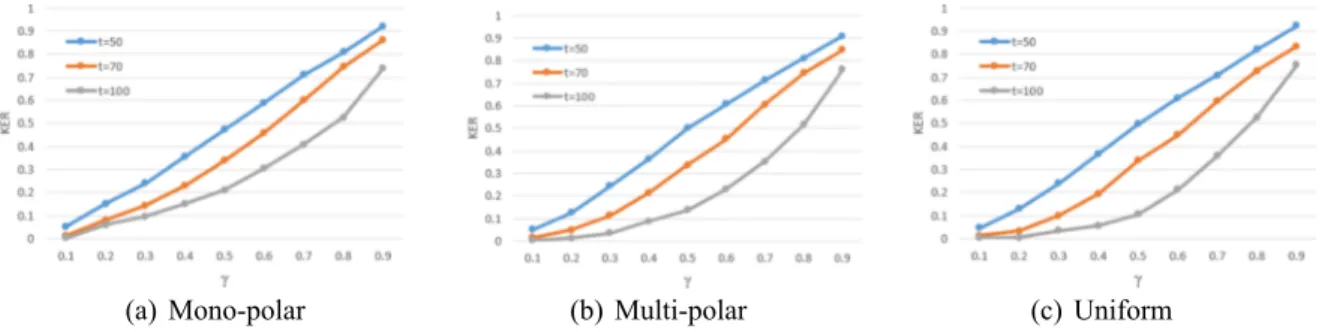
4.5. KPIs for core solutions

Having chosen several different location models allows us to explore the similarity of the solutions they provide (in terms of located

facilities) for any specific instance. We define a core solution N

(

t) as the set of locations i ∈ N such that y

=

1 in the optimal solution of

at least t% of the considered models. Then, the following KPI can assess the importance of a core solution:

•

RELATIVE IMPORTANCE OF CORE LOCATIONS

KER := |N

(

t)|/|N|

(50)

represents the proportion of locations included in the core solution for the total number of locations, given a threshold t.

Note that, in addition to the possible insights concerning a location model choice’s criticality, identifying a core solution might

decrease the computational burden for solving the problem itself. For example, the well-known Kernel Search metaheuristic (see, e.g.,

Angelelli et al., 2010; Manerba et al., 2018

, or

Gobbi et al., 2019

) is based on the concept of a core solution, that is, the set of variables

that have a larger probability of appearing with a non-null value in the optimal solution.

5. Experimental analysis

In this section, we first present the dataset generation procedure and then discuss the experimental results obtained. All the models

have been solved optimally by using Gurobi v8.1.0. The computer used for the experiments is an Intel(R) Core(TM) i7-5500U

CPU@2.40 GHz with 8 GB of RAM and running Ubuntu v18.04. However, we are not interested in analyzing the computational

performances of the different models in detail; furthermore, the solving times are almost negligible, considering the location decisions’

strategic level. To summarize, the time to solve a back-up model never exceeds 1 s of CPU time, and the most time-consuming model

seems to be the p-median for a small number of facilities to locate (approximately 15–20 s). In conclusion, given a specific case, the

entire set of the models we consider can be solved, and the entire set of KPIs can be calculated in less than 30 s.

5.1. Generation of test datasets

As our goal was to validate our approach, rather than apply it to a specific problem or real-case, we generate a broad set of random

instances simulating realistic scenarios as follows.

in-ternal distance d

for each node i ∈ N is generated as d

=

θ

*min

d

, where θ is a random variable uniformly distributed in [0,1].

Thus, we ensure that the internal demand can be best satisfied by locating a facility in the same node. Each node’s coordinates are

drawn according to specific probability distributions on a [ − 10, 10] × [ − 10, 10] square. Clearly, by changing the distributions and

their parameters, we can generate datasets with different specific features. In particular, we created three types of datasets with the

following characteristics:

•

mono-polar: datasets that simulate the case of a region where a single main cluster of demand nodes exists, in addition to few

sparse nodes around it (e.g., a district where there is one large city and other tiny satellite municipalities). The coordinates of 80%

the nodes are drawn from a Student’s t distribution with 3 degrees of freedom, and those of the remaining 20% are drawn from a

Uniform distribution;

•

multi-polar: datasets that simulate the case of a region where there exist several dispersed clusters of demand nodes (e.g., a district

with small-medium cities of similar sizes). The nodes’ coordinates are drawn from a sum of independent Multinomial distributions

with random mean value and a unit standard deviation;

•

uniform: datasets that simulate the case of a region where there is no cluster of demand nodes and the nodes are all dispersed (e.g.,

an urban area where the demand is spread uniformly across the region). The coordinates of the nodes are drawn according to a

Uniform distribution.

An example of the dispersion of the nodes in each type of dataset is shown in

Fig. 1

.

Then, the demand Q

for each node i ∈ N is generated randomly. Notice that, because both the models and the KPIs are based only

on the demand rate h

, the exact values of Q

do not influence the analysis.

Finally, to simulate different possible situations, we consider p = |N|*γ facilities to locate and a coverage radius d such that P[D <

d] =

μ

, where D is the random variable based on which the distances between two nodes are generated. In other words, d represents the

μ

-th percentile of the distances. For each one of the three types of datasets above and for every combination of γ = {0.15, 0.30, 0.45,

0.60} and

μ

= {

0.1,0.3,0.5}, we generate 10 different datasets. This means we have a total of 360 different datasets.

5.2. Results and discussion

Our discussion of the results is divided into four main parts: a comparison of the proposed models through the selected topological

and coverage KPIs (Section

5.2.1

), through the equity KPIs (Section

5.2.2

), through the ad-hoc KPIs for progressive interventions

(Section

5.2.3

), and an analysis of the core solutions (Section

5.2.4

).

5.2.1. Model comparison through topological and coverage KPIs

In this section, we discuss the performance of the different location models for the selected topological and coverage KPIs, for

different values of the coverage radius d, the number of facilities to locate p, and type of dataset. We calculate their relative absolute

deviation (RAD) from the best possible values to compare all KPIs. Since we are considering service facilities, such benchmarks are

computed for each dataset by simply fixing y

=

1, ∀i ∈ N (i.e., all the nodes are located). This means that the RADs for all the KPIs

indicate a better performance when they are closer to 0. Note that for some KPIs (namely, all the topological ones except Disp and Acc),

the benchmark solution provides the minimum possible values. In contrast, for the remaining KPIs, opening a facility in all the

lo-cations provides the maximum possible values. Finally, it is important to notice that, although each KPI has a possibly different

dimension, RADs are dimensionless because they are relative to the corresponding benchmarks.

In

Tables A.7–A.15

from

Appendix A

, for each combination of the value of

μ

(defining the coverage radius) and type of datasets

(mono-polar, multi-polar, and uniform), we present the average RADs of each KPI over the 10 generated datasets. Each row is uniquely

identified in these tables by the model used (Model) and the percentage (γ) of facilities to locate. Then, there is a specific column for

each topological and coverage KPI. For the BACOP1, we calculate the average RADs of the KPIs only for datasets where a feasible

solution exists (we report the number of feasible solutions out of 10 in square brackets next to the model name in the first column).

When no feasible solution exists for all the datasets, we report “NAN” for each KPI. However, note that infeasibility affects only two

entries in the first table, and therefore, does not bias the general comparisons.

Such detailed results are very hard to read. Therefore, in the following, we propose some ad-hoc aggregate views over all the

combinations of KPIs,

μ

, and γ to find some clear trends in the results:

•

average of RADs: since the goal of our analysis is to be as general as possible, we assume that all the KPIs have the same importance,

and therefore we consider their simple average. It is worth noting that, since RADs may have very different magnitudes (as in our

case), such an aggregate view may present big standard deviations;

•

percentage of times that a model provides the best RAD (WIN): this aggregate view looks at estimating the probability that a model

achieves the best value of a specific KPI

•

percentage of times that a model provides the top three RADs (PODIUM): this aggregate view looks at estimating the probability

that a model performs in the top three models of a specific KPI, i.e., it takes into considerations more performance dynamics

concerning the WIN aggregator;

Table 1

Averages and standard deviations of RADs for topological KPIs across all datasets.

RADs Mono-polar Multi-polar Uniform Tot Avg

avg stdev avg stdev avg stdev avg stdev

p-center 16.61 21.50 12.81 16.43 6.27 7.43 11.90 15.12 p-median 17.23 24.67 10.53 13.00 6.23 6.94 11.33 14.87 p-centdian 15.89 20.90 11.57 13.84 6.21 7.20 11.23 13.98 MCP 19.89 25.68 14.16 16.42 8.31 9.99 14.12 17.36 BACOP1 15.81 18.15 18.31 22.54 8.29 9.73 14.09 16.77 BACOP2-0.01 25.34 37.58 17.95 18.93 15.61 17.45 19.64 24.65 BACOP2-0.25 24.94 37.15 17.11 18.02 15.55 17.36 19.20 24.18 BACOP2-0.50 23.65 34.51 16.59 17.13 15.26 17.08 18.50 22.90 BACOP2-0.75 21.16 29.29 16.51 17.15 14.98 16.71 17.55 21.05 BACOP2-0.99 20.48 27.53 16.25 16.71 13.82 15.84 16.85 20.03 Tot Avg 20,18 27,74 16,98 20,20 7,95 9,37 15,02 19,08 Table 2

Averages and standard deviations of the RADs for coverage KPIs across all datasets.

RADs Mono-polar Multi-polar Uniform Tot Avg

avg stdev avg stdev avg stdev avg stdev

p-center 0.81 1.11 0.63 0.83 0.55 0.50 0.66 0.81 p-median 0.87 1.27 0.55 0.56 0.55 0.52 0.66 0.78 p-centdian 0.78 1.01 0.65 0.86 0.54 0.50 0.66 0.79 MCP 0.79 1.11 0.70 0.93 0.53 0.55 0.67 0.87 BACOP1 0.77 1.20 0.74 0.97 0.60 0.71 0.70 0.95 BACOP2-0.01 0.81 1.31 0.81 1.00 0.85 0.98 0.82 1.10 BACOP2-0.25 0.83 1.35 0.81 1.01 0.85 0.98 0.83 1.11 BACOP2-0.50 0.66 0.87 0.83 1.05 0.84 0.95 0.78 0.96 BACOP2-0.75 0.70 0.96 0.82 1.03 0.83 0.94 0.78 0.98 BACOP2-0.99 0.64 0.83 0.73 0.85 0.82 0.94 0.73 0.87 Tot Avg 0.73 1.19 0.64 0.92 0.50 0.57 0.62 0.89 Table 3

Averages and standard deviations of the WINs for topological KPIs across all datasets.

WINs Mono-polar Multi-polar Uniform Tot Avg

avg stdev avg stdev avg stdev avg stdev

p-center 11.46 1.31 11.46 1.31 6.25 0.39 9.72 1.01 p-median 29.17 8.51 34.38 11.82 46.88 21.97 36.81 14.10 p-centdian 10.42 1.09 4.17 0.17 1.04 0.01 5.21 0.42 MCP 3.13 0.10 13.54 1.83 16.67 2.78 11.11 1.57 BACOP1 10.42 1.09 8.33 0.69 2.08 0.04 6.94 0.61 BACOP2-0.01 7.29 0.53 10.42 1.09 5.21 0.27 7.64 0.63 BACOP2-0.25 7.29 0.53 6.25 0.39 9.38 0.88 7.64 0.60 BACOP2-0.50 8.33 0.69 9.38 0.88 12.50 1.56 10.07 1.05 BACOP2-0.75 2.08 0.04 1.04 0.01 0.00 0.00 1.04 0.02 BACOP2-0.99 10.42 1.09 1.04 0.01 0.00 0.00 3.82 0.37

•

average scoring of a model (SCORE): for each model, it is associated with a score according to its ranking position concerning the

goodness of the RAD for a specific KPI (the better the model, the higher the score). Our scoring goes from 9 to 0, with step 1, since

we are considering ten models.

It is important to notice that the decision-maker may consider several other aggregate views, particularly those resulting

statis-tically robust in the specific case. Moreover, the view we propose can be calibrated in several ways to cope with real application

peculiarities. For instance, the aggregators can be calculated by selecting the most important KPIs for the application at hand. The

averages can be computed by weighting the KPIs with their relative importance, or different scoring functions can be adopted. In the

following, we analyze in detail the average RADs and the WIN aggregators, while we just report the results obtained for PODIUM

(

Tables B.19–B.21

in

Appendix B

) and SCORE (

Tables C.23–C.24

in

Appendix C

) aggregators.

In

Tables 1 and 2

we report, for each model, the overall average and standard deviation over the RADs of all the topological and

coverage KPIs, respectively, for all the datasets of a given type (mono-polar, multi-polar, and uniform). The total averages are also

shown in bold font. Furthermore, with the same layout, we also present in

Tables 3 and 4

the WIN aggregator results for topological

and coverage KPIs, respectively. As the reader can notice, these last two tables do not show the average by column because it is always

equal to 100%.

First, note that the average RADs across all the models (last row of

Tables 1 and 2

) clearly vary depending on the type of datasets.

For both types of KPIs, mono-polar and multi-polar datasets tend to be worse on average in terms of errors for the benchmark and

exhibit more evident differences in the models’ performance. In particular, the mono-polar datasets seem to be the worst-performing

ones for most models; however, some models perform worse in the multi-polar or the uniform case. Uniform datasets, except for a few

models, appear to be much easier to deal with in topological and coverage KPIs. This seems to depend on the particular topology of the

instances, in which central and peripheral nodes are differently distributed. In particular, peripheral nodes deteriorate most of the

KPIs’ values because they are distant from the others and thus require ad-hoc facilities to be well served. Therefore, the bad

perfor-mances of all the methods on mono-polar instances depend on their number of peripheral nodes that are not negligible (as in uniform

instances) and far from the high-density region (as in multi-polar instances). Instead, the distribution used in uniform instances ensures

an average density of the nodes that guarantees a better homogeneity in the solutions of different models and, in turn, in the KPIs value.

Second, we compare the behavior of different models. Concerning the topological KPIs (

Table 1

), three different levels of

per-formance can group models. In the best group, containing p-center, p-median, and p-centdian, the latter is the best model, both in

terms of average and standard deviation. However, the model is not outperforming p-center and p-median, which show only slightly

worse performances. This is not surprising since p-center, p-median, and p-centdian have objective functions considering topological

properties. The second group contains MCP and BACOP1, which behave similarly and perform three points worse than the first group.

Finally, the third group includes all the BACOP2 models, which perform 2–5 points worse than the second group. A clear trend is that

the higher the

α

, the better the results. The difference in the performance of BACOP2 models may be due to their objective functions,

which do not consider topological features of the solution. It is noteworthy that, apart from the total averages, BACOP1 performs better

than the other models in the mono-polar datasets, whereas p-median performs better than the other model in the multi-polar datasets.

By looking at the WINs results for topological KPIs in

Table 3

, p-median achieves the best performance, followed by MCP, BACOP2-

0.50, and p-center. Instead, on average, BACOP2-

α

with high values of

α

and p-centdian show the worst results. These models also

show a significant difference in performance concerning the instances type, making them very bad for uniform instances.

Regarding the coverage KPIs, some similar trends can be detected in the RADs results of

Table 2

, even if the differences between the

models are not that evident. p-centian, p-center, and p-median still have the best averages. However, in this set of KPIs, the MCP

performance is only slightly worse than that of the best model (outperforming BACOP1). Again, among the BACOP2 models, the best

results are obtained for the higher values of

α

. It is worth noting that BACOP2-0.99 (which performs quite severely in the uniform case)

is the best choice for mono-polar datasets. p-median is still the best model for multi-polar datasets. In contrast, MCP is the best model

for uniform datasets. From the WINs results shown in

Table 4

, we can derive that p-center has the best performance, followed by MCP.

It is essential to notice that all the other models rarely achieve the best results. If compared with the previous results on topological

KPIs, we can enforce the role of p-center while probably MCP should be better considered. The latter achieves the best results several

times, which means that the second-class performance obtained on the topological KPIs is probably due to few but awful values in the

Table 4

Averages and standard deviations of the WINs for coverage KPIs across all datasets.

WINs Mono-polar Multi-polar Uniform Tot Avg

avg stdev avg stdev avg stdev avg stdev

p-center 41.67 17.36 81.25 66.02 81.25 66.02 68.06 49.80 p-median 0.00 0.00 2.08 0.04 0.00 0.00 0.69 0.01 p-centdian 0.00 0.00 0.00 0.00 6.25 0.39 2.08 0.13 MCP 56.25 31.64 16.67 2.78 12.50 1.56 28.47 11.99 BACOP1 2.08 0.04 0.00 0.00 0.00 0.00 0.69 0.01 BACOP2-0.01 0.00 0.00 0.00 0.00 0.00 0.00 0.00 0.00 BACOP2-0.25 0.00 0.00 0.00 0.00 0.00 0.00 0.00 0.00 BACOP2-0.50 0.00 0.00 0.00 0.00 0.00 0.00 0.00 0.00 BACOP2-0.75 0.00 0.00 0.00 0.00 0.00 0.00 0.00 0.00 BACOP2-0.99 0.00 0.00 0.00 0.00 0.00 0.00 0.00 0.00