https://doi.org/10.1007/s10018-020-00294-3
RESEARCH ARTICLE
Accounting for adaptation and its effectiveness
in International Environmental Agreements
Francesco Furini1,3 · Francesco Bosello2,3,4,5 Received: 24 June 2020 / Accepted: 23 October 2020 © The Author(s) 2020
Abstract
This paper analyses, within a standard International Environmental Agreement game, the effect of the introduction of adaptation on climate negotiation. The model expands the existing literature by considering a double relation between the two strategies. The common assumption that higher mitigation decreases the marginal benefit of adaptation and vice versa is enriched allowing for the possibility that mitigation, leading to lower and more manageable damages, determines a greater effectiveness of adaptive measures. We find the possibility for adaptation and miti-gation to be strategic complements and not, as commonly believed, substitutes. Yet, as already known from the literature, the presence of adaptation can determine upward-sloping mitigation reaction functions regardless of the strategic relationship between mitigation and adaptation. When this is the case, the grand coalition can form. Nonetheless, large participation can induce substantive welfare gains only if adaptation and mitigation are strategic complements.
Keywords Climate change · Adaptation effectiveness · Mitigation-adaptation strategic relation · International environmental agreements game
Electronic supplementary material The online version of this article (https ://doi.org/10.1007/s1001 8- 020-00294 -3) contains supplementary material, which is available to authorized users.
* Francesco Furini
[email protected] Francesco Bosello
1 Department of Socioeconomics, Universität Hamburg, Hamburg, Germany
2 Department of Environmental Science and Policy, Università Statale Milano, Milan, Italy 3 Department of Environmental Sciences, Informatics and Statistics, Università Ca’ Foscari
Venezia, Venice, Italy
4 Centro Euro-Mediterraneo sui Cambiamenti Climatici (CMCC), Venice, Italy
JEL Classification C71 · D62 · D74 · F53 · H41 · Q54
1 Introduction
Combating climate change is increasingly recognized as one of the key challenges that our society has to address. The two pillars of climate change policy are mitiga-tion and adaptamitiga-tion. The former acts directly on the cause of the problem, reducing emissions and lowering future climate change. The latter acts on its consequences tackling directly climate impacts. Recognizing the global public bad nature of cli-mate change, the international community started since the beginning of the 90 s a complex negotiation process under the umbrella of the United Nation Framework Convention on Climate Change to set and coordinate an equitable, effective and effi-cient climate action.
These negotiations rounds offered a natural and extremely fertile ground to apply game and coalition theory models. These have been amply used to predict the poten-tial outcomes of international negotiations on climate change and, in particular, to explain the very reason behind the unsatisfactory achievement of “large” coopera-tion or of “substantive” environmental effectiveness. The first stream of literature on International Environmental Agreements (IEAs), however, has largely focused on mitigation, while adaptation has been somewhat overlooked. The general result of this literature is that a large (with many countries) and stable (without internal defeaters or external entrants) coalition is not possible to obtain (Hoel 1992; Car-raro and Siniscalco 1993).1 The driver of the outcome is the incentive to free ride.
Intuitively: when, or exactly because, the agreement produces large environmental benefits (it is stringent), then the incentive to free ride by single players is too strong to be possibly offset by the remaining members of the coalition. Thus, the coali-tion shrinks until the incentive to free ride becomes sufficiently small. This typically occurs when few members (two or three) are left. There is a “dual” interpretation of this exit: when large coalitions do form, it is because the underlying agreements entail a low incentive to free ride, i.e., they are close to a “do nothing” business as usual.
In the last decade, a more recent stream of literature emerged studying the inter-play between mitigation and adaptation in IEAs. This crop of papers is mostly based on empirical Integrated Assessment Models with only few proposing theoretical framework (Zehaie 2009; Ebert and Welsch 2011 and 2012; Ingham et al. 2013; Eisenack and Kahler 2016). Even fewer have analyzed how the presence of adapta-tion could affect the size and stability of an IEA (Benchekroun et al. 2011; Buob and Siegenthaler 2011; Marrouch and Chaudhuri 2011; Auerswald et al. 2018; Bayra-moglu et al. 2018; Breton and Sbragia 2019).
1 The literature on IEA games has extended over the years. Finus and Caparrós (2015) provide a collec-tion of some of the most influential papers on the topic. Many aspects of climate negotiaa collec-tion are analyzed and, in some cases, more optimistic conclusions are achieved (see, for instance, Barrett and Dannenberg 2012, Eyckmans and Finus 2007 and Finus and Maus 2018).
The presence of adaptation might indeed change the nature of the emissions reduction game, acting on the incentive to free ride. The intuition is that, if adapta-tion is possible, the optimal reply to a potential free rider to a climate agreement could be more adaptation and not more mitigation. This could reduce the free riding benefit and, thus, foster the stability of a climate coalition. Ebert and Welsch (2011
and 2012), analytically show in a 2-player context the possibility for upward-sloping emissions reaction functions, i.e., complementarity between emissions strategies, when adaptation is included as a strategy to fight climate change. Upward-sloping reaction functions would transform a “leakage game” into an emissions (mitigation) “matching game” and could favor the stability of climate coalitions.
This issue has been extensively examined by Bayramoglu et al. (2018). The paper examines the effect of adaptation on the strategic interaction among players’ mitiga-tion decisions and on stable coalimitiga-tion size. Both substitutability (standard case) and complementarity (special case) across strategies are assumed. One of the interesting points of the paper is that upward-sloping mitigation reaction functions occur when the adaptation–mitigation interaction is “sufficiently large”, regardless of whether the two strategies are complements or substitutes. When mitigation reaction func-tions are upward sloping, participation to a climate agreement increases. The authors find that in a game where only mitigation is an option, and hence with downward-sloping reaction functions, the stable coalition size will be at most 2. Instead, when adaptation is an option and it leads to upward-sloping mitigation reaction functions, the stable coalition size will be larger or equal to 3.
The strategic relation between mitigation and adaptation has been examined by a parallel stream of literature, concluding that whether the two are complements or substitutes is mostly an empirical matter. Adaptation and mitigation are commonly seen and modeled as economic substitutes: if the cost of mitigation falls (rises), then the optimal response is to increase (decrease) the level of mitigation and decrease (increase) the level adaptation. However, for instance, Ingham et al. (2013) show that, when adaptation costs depend on the amount of mitigation, the two strategies can be complements. This can occur if adaptation were harder to implement under faster rates of climate change. By reducing emissions, countries not only reduce the rate of climate change, but also facilitate (buy time for) adaptation. As assumed by Ingham et al. (2013), adaptation and mitigation may be linked by more than one relationship and as a result, the standard assumption of strategic substitutability may be reversed.
Building on this idea, the purpose of this paper is to further investigate the inter-connections between mitigation and adaptation and the effects that they could have on climate negotiation outcomes.
Our starting point is Bayramoglu et al. (2018), whose analysis we enrich insert-ing a double connection between adaptation and mitigation.2 The first is the standard
one: higher levels of adaptation, reducing the marginal damage from climate change, weaken the benefits from mitigation. Conversely, higher levels of mitigation, by
2 Hence, our modification is introduced in the game that considers both mitigation and adaptation, while the pure mitigation game does not change from Bayramoglu et al. (2018).
generating less damages to be attenuated, reduce the incentive for protection. The second is similar in spirit to Ingham et al. (2013). Specifically, we include an adap-tation effectiveness parameter that depends on total mitigation level so that higher mitigation determines higher productivity of adaptation, an issue not yet consid-ered in the analysis of climate coalition formation. This assumption finds support in the scientific literature. The IPCC AR4 (IPCC 2007) states that as climate change increases, not only do the costs increase but also the options for successful (we read effective) adaptation diminish. Adaptation effectiveness appears closely linked to the rate and magnitude of climate change according to Adger et al. (2007) while Romero-Lankao et al. (2014) state that “several lines of evidence indicate that effec-tive adaptation requires changes in approach and becomes much more difficult if warming exceeds 2 °C above preindustrial levels”.
Some practical, although speculative, examples can be provided. The first can be related to “catastrophic damages” and the concept of “adaptation tipping points”, i.e., situations in which policies are no longer able to achieve their objectives (Van Ginkel et al. 2020). A typical case is when coastal (or river flood) protection fails due to “too high” and/or “too rapid”, “too frequent” flood events. In this specific case, the presence of hard adaptation measures may even worsen the damage, as water would be more difficult to be removed from the flooded areas. In our con-text: if “more mitigation” were able to keep the damage below the adaptation tipping point, then adaptation effectiveness would be greatly improved. The reasoning can be extended also to “continuous” or “slow on set” climate damages if we agree upon the idea that adaptation is eventually a “technology” that operates with “standard” diminishing marginal and scale returns. Examples here could be more easily found in the case of “reactive” adaptation. For instance, even though within the range of coping capacity, health care systems can work better at low rather than high levels of congestion. Similarly, interventions against forest fires can be more effective if fire episodes are few rather than many. In both situations, more resources could be con-centrated on specific emergencies to pursue the desired outcome.3 We claim that this
situation—productivity of adaptation related to mitigation level—is in fact the usual one and, as such, should be taken into account to increase the realism of the analysis of the two strategies.
With this enriched modelling, we show that the possibility emerges for adapta-tion and mitigaadapta-tion to be complements and not, as commonly believed, substitutes. Our new assumption also alters the effect that adaptation has on mitigation strate-gies. In our setting the possibility for upward-sloping mitigation reaction functions, is in fact less likely than in Bayramoglu et al. (2018). This happens because, in our case, mitigation entails a double positive externality (it reduces climate damages and it increases adaptation effectiveness), making the incentives to free ride stronger. Finally, we introduce explicit payoff functions to analyze stable coalition size and their welfare performances. Differently from Bayramoglu et al. (2018) (stable
3 Note that, here, we do not refer to the efficiency scale of adaptation, but just to the effectiveness. In principle, a health care system can be over-sized compared to the patients to treat which can lead to inef-ficiency.
coalition size larger or equal to 3 with upward-sloping reaction function), we find that stable coalition size will be either 3 or the grand coalition (full cooperation). This result is in line with Rubio (2019). Regarding welfare: when stable coalitions are small, welfare improvements compared to non-cooperation are also small. When the grand coalition forms, welfare gains compared to non-cooperation are small if the two strategies are substitutes. This confirms a consolidated finding from the ‘90 s literature on the topic. However, if the two strategies are complements, the grand coalition will bring large welfare improvements compared to non-cooperation.
In what follows: Sect. 2 introduces the game theoretical model and its general assumptions, Sect. 3 describes the climate negotiation process as a multi-stage game, Sect. 4 solves the game presenting major results, and Sect. 5 concludes. 2 The model
We consider n symmetric players (countries) i = 1, 2, ..., n , and 2 different games. In the pure mitigation game (M-Game), our reference, players can only use emis-sions reduction as a strategy to combat climate change. Adaptation is introduced in the mitigation–adaptation game (M + A-Game). In the M-Game, we adopt the same general payoff function of Bayramoglu et al. (2018) given by:
In the M + A-game, we introduce a substantial modification, with the payoff func-tion given by:
The total welfare will be the sum of all individual payoffs W = ∑n i=1wi.
In the M-Game (function 1a), individual payoff is given by the benefit Bi from
total mitigation M = ∑n
i=1mi , minus the cost Ci of individual mitigation mi . In
the M + A-Game (function 1b), benefits depend on total mitigation M , individual adaptation ai and its effectiveness 𝜀 that is a function of total mitigation. The cost
functions Ci(mi
)
and Di(ai
)
depend, respectively, on the individual mitigation and adaptation levels. Every player i in the M-Game will decide its level of individual mitigation mi∈[0, mi
]
, while in the M + A-Game, it will also set its individual adap-tation level ai∈[0, ai
] .
Players have identical individual payoff functions and, thus, are assumed to be ex ante symmetric. However, as it will be clear below, in the first stage of the game, countries endogenously decide whether to be part of a climate coalition and become signatories or to remain outside as non-signatories. Signatories and non-signatories, (1a)
wi(M, mi) = Bi(M) − Ci(mi)
(1b)
face two different maximization problems leading to different mitigation levels. Accordingly, countries might be ex post asymmetric. This will happen when a non-empty coalition, that does not include all players, forms in the first stage of the game.4 Where appropriate, we stress this ex post asymmetry using the indexes S for
signatories and NS for non-signatories.
All payoff functions are assumed to be continuous with continuous first and second derivatives. Then, the following general assumptions on payoff functions are introduced.5 The subscripts refer to the kind of the derivative, e.g., B
M= 𝜕B 𝜕M , BMM = 𝜕2B 𝜕2M and BMa= 𝜕2B 𝜕M⋅𝜕a. General assumptions M-Game: M + A-Game: (ai) BM= BM+ B𝜀⋅ 𝜀M>0, BMM<0, Cm>0, Cmm>0. (bi) lim M→0BM>m→0limCm>0. (c) Ba>0, Baa≤0, Da>0, Daa>0, (d) lim
a→0Ba >lima→0Da>0.
Adaptation–mitigation strategic interaction
(e) 𝜀M>0, 𝜀MM ≤0.
(f) B𝜀>0, 𝜀MM ≤0, B𝜀M= B𝜀𝜀⋅ 𝜀M≤0,
(g) BaM= BMa<0.
(h) Ba𝜀= B𝜀a>0.
(i) BaM= BMa><0.
With, in assumption (ai):BMM=
𝜕(BM(M,ai,𝜀(M))+B𝜀(M,ai,𝜀(M))⋅𝜀M(M)) 𝜕M = BMM+ BM𝜀⋅ 𝜀M+ 𝜀MM⋅ B𝜀+ B𝜀M⋅ 𝜀M<0, with B𝜀M = 𝜕B𝜀(M,a,𝜀(M)) 𝜕M = B𝜀M+ B𝜀𝜀⋅ 𝜀M= 2B𝜀𝜀⋅ 𝜀M,
and, in assumption (i):
Assumptions (a), (ai), (c) and (f) set the standard properties of concave benefit and convex cost functions. This configuration guarantees, together with assumptions (b), (bi) and (d), strictly positive mitigation and adaptation equilibrium levels in both games. BM>0, BMM<0, Cm>0, Cmm>0, lim M→0BM>m→0limCm>0. BaM= 𝜕(Ba(M, ai, 𝜀(M) )) 𝜕M = BaM+ Ba𝜀⋅ 𝜀M= BMa= 𝜕(BM(M, ai, 𝜀(M)) + B𝜀(M, ai, 𝜀(M) ) ⋅ 𝜀M(M) ) 𝜕a = BMa+ B𝜀a⋅ 𝜀M><0.
4 If no coalition forms, all players would behave as non-signatories; while if the grand coalition forms, i.e., if all players join the coalition, everyone will behave as a signatory. In these two situations, countries will be both ex ante and ex post symmetric.
Assumptions (a), (ai) and (c) also describe the nature of mitigation and adapta-tion. Mitigation is a pure public good, as the marginal benefits are affected by total mitigation and not only by individual one. Adaptation is instead a private good: its marginal benefits depend only on individual adaptation levels. Assumptions (e–i) describe the strategic interaction between mitigation and adaptation. Assumption (e) represents the new element of this theoretical work. Adaptation effectiveness is defined as an increasing concave (or linear) function of total mitigation level. The logic behind this assumption is the idea that adaptive measures cannot be equally applied regardless of the damage level. In case of catastrophe, adaptation cannot be applied: even with an extreme effort, the damage cannot be substantively attenu-ated. Mitigation allows to avoid extreme damages and, as emissions decrease and climate change slows, adaptation starts to be increasingly effective. In this context, 𝜀 sets the amount of damage that can be avoided through adaptive measures. It can be conceived as a 0–1 variable: for example, value 1 would mean that the damage could be completely absorbed by adaptation, while with a value of 0.5 damage could be reduced by the 50%. The smaller the severity of damages, the larger the portion that can be eliminated by adaptation. This is what assumption (e) captures.
Assumption (g) confirms the standard mitigation–adaptation trade-off: higher lev-els of adaptation reduce the marginal benefit of mitigation and vice versa. Assump-tion (h) says that higher mitigaAssump-tion determines higher effectiveness of adaptive measures. This in turn increases marginal benefits from adaptation. The sign of the overall resulting adaptation–mitigation cross derivative (BaM= BMa) , indicated in assumption (i), is uncertain and is given by the sum of these two effects, the first one negative (BaM= BMa<0
)
and the second one positive (Ba𝜀⋅ 𝜀M= B𝜀a⋅ 𝜀M>0
) . 3 Climate change negotiations as a 2‑stage coalition formation
game
The International Environmental Agreement game is typically solved as a 2-stage game where countries choose whether to participate or not in a mitigation coalition in the first stage and set their level of mitigation (in the M-game) or of both mitiga-tion and adaptamitiga-tion (in the M + A-game) in the second stage.
Countries who join the coalition P in the first stage are the signatories (S); other countries are the non-signatories (NS). The size of coalition P is indicated by p . At the end of the first stage, p signatories will be part of the coalition and n − p non-sig-natories will be the outsiders. If,p = n the grand coalition (full cooperation) forms, and there will be no outsiders. In an externality game, this always represents the social optimum (SO). If p = 1 , the non-cooperative Nash equilibrium (NE) forms, and there will be no signatories. We refer to all other coalition sizes 1 < p < n as partial cooperation.6
6 It is in the case of partial cooperation, i.e.,
1<p < n , that we observe ex post asymmetry. In this case, we have p >1 signatories and n − p >0 non-signatories. The two groups will face different maximiza-tion problems.
In a game with a positive externality, a necessary condition for coalition for-mation is profitability. The coalition of size p is profitable if each signatory gets a higher payoff inside the coalition rather than in a non-cooperative Nash equilibrium. Formally, profitability can be written:
In the presence of free riding incentives, profitability is not a sufficient condition for the formation of a climate agreement. Stability is also needed. According to the majority of IEAs literature, here, we use the open membership rule (D’Aspremont et al. 1983), i.e., players can join and leave the coalition without the consensus of others. Consequently, stability should be both internal and external.
Internal stability requires that none of the signatories would be better off leaving the coalition P, while other players stay in the coalition. External stability requires that none of the non-signatories would be better off joining the coalition. Formally, internal stability can be written:
while external stability is:
When profitability, internal and external stability are jointly satisfied the coalition can be formed.7 For every coalition P , we allow for a unique equilibrium vector of
mitigation (mitigation and adaptation) decisions to exist. We introduce the unique-ness and existence condition in the next section.
In the second stage of the game, the coalition acts as a single player maximizing its payoff and internalizing the positive externality arising from mitigation. In the M-Game, signatories will choose the level of mitigation that maximizes their aggre-gate payoff, while each non-signatory will instead choose the mitigation level max-imizing its individual payoff. In the M + A-Game, signatories and non-signatories simultaneously set their mitigation and adaptation levels or, equivalently, they first set their mitigation levels and then, in a second step, adaptation levels.8
Hence, in both games, in the second stage of the game, players will maximize different objective functions depending on whether they are signatories or non-sig-natories. Signatories will maximize their aggregate welfare. Their objective function will be:
wS(p) > wNE.
(2)
w∗S(p) ≥ w∗NS(p −1),
w∗NS(p) ≥ w∗S(p +1).
8 The equivalence of the two games can be easily derived from the FOCs of the M+A-Game, and the demonstration is identical to Bayramoglu et al. (2018), thus we omit it. Final equilibrium levels will be the same as long as adaptation is not chosen before mitigation. The strategic role of anticipatory adapta-tion has been studied, in a 2-player context, by Zehaie (2009) and, with coaliadapta-tion formaadapta-tion, by Breton and Sbragia (2019).
7 Section 4.2.2 introduces specific welfare functions for both the M- and M+A-Game to analyze the first stage of the game. Indeed using generic welfare functions, it is not possible to derive conclusions on the size, mitigation and welfare of stable coalitions.
The p signatories are symmetric and act cooperatively. The total mitigation level
M can be written as the sum of mitigation levels of the p signatories and of the n − p
non-signatories: M = p ⋅ mS+ MNS with MNS=[n − p]⋅ mNS . The objective
func-tion of signatories can be written as: in the M-Game and
in the M + A-Game.
Non-signatories will maximize their individual welfare non-cooperatively. Hence, the objective functions of the n − p non-signatories will coincide with their individual welfare functions: ObjM
NS = (1a) in the M-Game and Obj M+A
NS = (1b) in the
M + A-Game.
4 Outcome of the mitigation and mitigation–adaptation game The game is solved by backward induction. We start from the second stage analyz-ing mitigation and adaptation first-order conditions, equilibrium levels and interde-pendencies, and then we move to the analysis of the first-stage coalition formation. 4.1 Second stage: mitigation and adaptation decisions
4.1.1 Preliminaries
In the second stage, after a coalition P has formed in the first stage, signatories and non-signatories choose their optimal strategies. In the mitigation game, signatories will choose their mitigation level to maximize their objective function (3a). Non-signatories will instead maximize their individual welfare (1a). In the M-Game, the first-order conditions are given by:
In the M + A-Game, signatories and non-signatories will maximize (3b) and (1b), respectively. Differentiating the objective functions with respect to individual miti-gation, the following FOCs are obtained:
ObjS=∑ p wS. (3a) ObjMS = p ⋅[BS(p⋅ mS+ MNS) − CS(mS)], (3b) ObjM+AS = p ⋅[BS(p⋅ mS+ MNS, aS, 𝜀(p⋅ mS+ MNS)) − CS(mS) − DS(aS )] (4a) Signatories ∶ p ⋅ BM(M) = Cm(mS). (4b) Non − signatories ∶ BM(M) = Cm(mNS).
Additionally, in the M + A-game, differentiating the objective functions (3b) and (1b) with respect to adaptation will lead to the following adaptation FOC, equal for both signatories and non-signatories:
These FOCs, enable to identify some relations between signatories and non-sig-natories in terms of mitigation, adaptation and welfare levels.
Lemma 1 (Mitigation, adaptation and payoff levels’ relations between signatories and non-signatories).
If a coalition of size p ≥ 2 has formed in the first stage, then the following holds:
Proof. see Appendix 1
The first and last statements hold for both games, while the second one, involving adaptation, only refers to the M + A-Game. The free ride incentive is well explained by the relations of Lemma 1 as non-signatories are better off than signatories in both M- and M + A-Game.
Mitigation FOCs (4a), (4b), (5a) and (5b) define players’ reaction functions in the mitigation space. Total mitigation is the individual mitigation level of player i,
mi, plus the mitigation of all other players, M−i : M = mi+ M−i . In this way, every mitigation FOC defines mi as a function of M−i . This is the individual reaction
func-tion of player i in the mitigafunc-tion space. In both M- and M + A-Game, we can identify the individual mitigation best response functions of signatories and non-signatories, respectively, as rS(M−i∈P
)
and rNS(M−j∉P
) .
Moving to adaptation, FOC (6) is equal for all players. Individual adaptation can be expressed as a function of total mitigation. This indicates the reaction functions in the adaptation space h(M) = a∗(M) that is equal for signatories and non-signatories.
A preliminary step of the analysis is to define the condition that guarantees to have a unique second-stage equilibrium. The following assumption needs to be satisfied.
Additional assumption (Existence and uniqueness conditions of a second-stage equilibrium). (5a) Signatories ∶ p ⋅[BM(M, aS, 𝜀(M)) + B𝜀(M, aS, 𝜀(M) ) ⋅ 𝜀M(M)] = Cm(mS). (5b) Non − signatories ∶[BM(M, aNS, 𝜀(M)) + B𝜀(M, aNS, 𝜀(M) ) ⋅ 𝜀M(M)] = Cm(mNS). (6) Ba(M, a) = Da(a). m∗S(p) > m∗NS(p), a∗S(p) = a∗NS(p), w∗S(p) < w∗NS(p).
In the M + A-Game, let ΨM+A= B MM+ ( BaM )2 Daa−Baa. If Ψ
M+A>0, then a unique
sec-ond-stage equilibrium exists if: ΨM+A
⋅ [ p2 Cmm(mS)+ (n−p) Cmm(mNS) ] <1.
Proof. see Appendix 1
4.1.2 General results
Proposition 1 (slopes of reaction functions in the mitigation space).
Let ΨM= B
MM for the M-Game and ΨM+A= BMM+
(
BaM)2
Daa−Baa for the M + A-Game.
Slopes of individual mitigation reaction functions of signatories and
non-signato-ries are, respectively, given by r�
S(M−i∈P) = C p⋅Ψ mm(mS)−p⋅Ψ and r� NS(M−j∉P) = Ψ Cmm(mNS)−Ψ.
Proof. See Appendix 1
In the M + A-Game, reaction functions can be upward sloping, and this will happen in our model when ΨM+A>0.
The substantive difference from Bayramoglu et al. (2018) stems from the term determining the slope of mitigation reaction functions in the M + A-Game. In Bayramoglu et al. (2018), it is defined as: AM+A= B
MM+
(BaM)2
Daa−Baa.
We can notice that “our” ΨM+A<AM+A . ΨM+A and AM+A are composed by a
negative term (respectively, BMM as defined in general assumption ai and BMM )
plus a positive term (respectively,
( BaM)2 Daa−Baa = (BaM+Ba𝜀⋅𝜀M) 2 Daa−Baa and (BaM) 2 Daa−Baa ). Comparing
the terms, the positive squared term of ΨM+A is lower than the one of AM+A as it is
composed by two compensating effects. The negative term is also smaller (more negative). Indeed, we have BMM <BMM by the definition of BMM . Therefore, in
our configuration, introducing adaptation effectiveness dependence on total miti-gation level increases the stringency of the condition to have upward-sloping mit-igation reaction functions in the M + A-game. Accordingly, if a country increases its mitigation commitment, it will be easier to be in the case where all other coun-tries react by reducing their mitigation levels. Intuitively, in our M + A-game, mitigation entails a double positive externality. On the one hand, all the players will receive a higher direct benefit from total mitigation; on the other hand, coun-tries will receive higher benefits from their adaptive measures as they will be more effective. Having a double positive externality, the free riding incentive will be higher and hence, mitigation levels will likely be strategic substitutes.
Now, endowed with our new assumption on adaptation effectiveness, we explicit the strategic relations between adaptation and mitigation, i.e., conditions for complementarity or substitutability.
Proposition 2 (Adaptation–mitigation strategic relation).
In the mitigation–adaptation space, the slope of each player’s reaction func-tion h(M) is given by h� (M) = 𝜕a 𝜕M = BaM Daa−Baa = BaM+Ba𝜀⋅𝜀M
Daa−Baa Then, mitigation and
adap-tation will be substitutes (complements) if BaM+ Ba𝜀⋅ 𝜀M<(>)0.
Proof. See Appendix 2
Proposition 2 sets the possibility to have strategic complementarity between miti-gation and adaptation. Strategic complementarity occurs when the positive term
Ba𝜀⋅ 𝜀M , originated by the dependence of adaptation effectiveness on mitigation,
dominates the standard negative interdependency BaM . This outcome is an
alterna-tive formalization of the findings of Ingham et al. (2013) in which complementarity could arise in the special case where adaptation costs were depending on the amount of mitigation.9
It is worth stressing an important implication of Propositions 1 and 2. As in Bay-ramoglu et al. (2018), it is the interaction between mitigation and adaptation that can determine upward-sloping mitigation reaction functions, but not the nature of the relation. In ΨM+A , the term B
aM = BaM+ Ba𝜀⋅ 𝜀M (which determine the nature
of interaction between mitigation and adaptation) is squared. Thus, upward-sloping mitigation reaction functions can occur either with complementary or substitute mit-igation and adaptation. What is needed is that the strategic relation is “sufficiently” strong (large value of BaM = BaM+ Ba𝜀⋅ 𝜀M in absolute terms).
This said, the strategic relation between adaptation and mitigation does play an important role on the final equilibrium levels of the M + A-Game. Compared to the pure mitigation game, we can conclude, in line with Bayramoglu et al. (2018): Corollary (Mitigation levels in the M-Game and in the M + A-Game).
Consider an arbitrary coalition of size p formed at the first stage of the game. At the second stage, if adaptation and mitigation are strategic substitutes (com-plements), then we will have mM+A
S (p) < (>)m M S(p), m M+A NS (p) < (>)m M NS(p) and MM+A(p) < (>)MM(p).
Proof: See Appendix 2
Complementarity or substitutability between mitigation and adaptation deter-mines the change in mitigation levels moving from the M-Game to the M + A-Game. When the two strategies are complements, for any given coalition size p , individual
9 Other studies in which adaptation and mitigation are found to be strategic complements are Yohe and Strzepeck (2004 and 2007). They focus on tipping points saying that, when impacts from climate change are ‘‘not smooth, non-monotonic and not manageable’’, adaptation–mitigation complementarity should be the rule and not the exception.
and total mitigation levels will be higher in the M + A-Game compared to the pure mitigation game. If they are substitute, mitigation levels will be lower.
Compared to Bayramoglu et al. (2018), we can also claim that, under the stand-ard assumption of substitutability, the introduction of the dependence of adapta-tion effectiveness upon mitigaadapta-tion, induces a lower decrease of mitigaadapta-tion levels in the M + A-Game. This is true for both signatories and non-signatories and, hence, applies to total mitigation as well (Appendix 2).
4.2 First stage of the game
In the first stage, players choose whether to join the mitigation coalition or not. This is the crucial stage of the game in which cooperation takes form.
4.2.1 General properties
To characterize the incentives to join a coalition P and to analyze the effect on coa-lition size, on second-stage mitigation and welfare levels we first introduce three properties of the game: positive externality property (PEP), superadditivity (SAD) and cohesiveness (COH). We refer to two dimensions of cohesiveness; the standard one that is the welfare dimension (WCOH), and the mitigation dimension (MCOH). Definition 2 Superadditivity, Positive externality, and Cohesiveness
(i) Superadditivity holds if, for every coalition size p ≥ 2 and for every i ∈ P :
p ⋅ w∗ S(p) ≥[p − 1]⋅ w ∗ S(p −1) + w ∗ NS(p −1) .
(ii) Positive externality property holds if, for every j ∉ P : w∗
NS(p) ≥ w
∗
NS(p −1).
(iii) Mitigation cohesiveness holds if for every coalition size p ≥ 2 and for every i ∈ P : p ⋅ M∗ S(p) + (n − p) ⋅ M ∗ NS(p) ≥[p − 1]⋅ M ∗ S(p −1) +[n − p + 1]⋅ M ∗ NS(p −1).
(iv) Welfare cohesiveness holds if, for every coalition size p ≥ 2 and for every
i ∈ P : p ⋅ w∗ S(p) + (n − p) ⋅ w ∗ NS(p) ≥[p − 1]⋅ w ∗ S(p −1) +[n − p + 1]⋅ w ∗ NS(p −1).
Superadditivity and positive externality are linked to stable coalition size. Look-ing to the internal stability condition (2), it is clear that superadditivity is a neces-sary condition for coalition stability. If coalition of size p is stable, then the move from p − 1 to p is superadditive. If we consider a coalition of size p = 2 , then SAD is a sufficient condition for its stability. If the move from p = 1 to p = 2 is superadd-itive, then the coalition p = 2 is internally stable. PEP refers instead at the positive externality generated by the coalition. It holds when the welfare of players outside the coalition benefit from an enlargement of participation. This property is an obsta-cle to the stability of large coalitions. As the coalition gets larger, the incentives to stay outside are bigger and therefore, the internal stability condition is more difficult to be satisfied.
If both SAD and PEP hold, then welfare cohesiveness holds as well. However, neither of the two cohesiveness properties are associated with coalition stability. They refer instead to the positive effect that higher participation to a climate agree-ment would have on total mitigation and welfare levels. When cohesiveness holds, larger coalitions would bring higher total mitigation (MCOH) and/or higher total welfare (WCOH). However, if they fail, larger coalitions would bring a loss in terms of total mitigation and/or welfare. For this reason, we should not only look at the number of participants in a mitigation agreement, but also which are the final miti-gation and welfare levels.10
Proposition 3 (general properties of the games) For what concerns the properties of
our pure mitigation and mitigation–adaptation game:
(a) SAD always holds when ΨM+A>0.
(b) PEP always holds in both games. (c) MCOH always holds in both games.
Proof: See Appendix 3
The general properties of the game do not differ from Bayramoglu et al. (2018). We now check how the enrichment of the relationship adaptation–mitigation affects three aspects: stable coalition size, mitigation levels and the welfare of coalitions.11
4.2.2 Explicit payoff functions
To investigate these aspects, we introduce explicit functional forms for the payoff of the two games; that of the M-Game is taken from Bayramoglu et al. (2018):
In the M + A-Game, the payoff function is instead given by:
(7) wMi =(bM −g 2M 2)− c 2m 2 i. wM+Ai = ( bM −g 2M 2)+ a(𝛽 + 𝜀 − fM) − c 2m 2 i − d 2a 2,
10 For cohesiveness properties, we do not focus on adaptation. In our model, it is directly related to total mitigation level and, therefore, we could link it to mitigation cohesiveness property. When total mitiga-tion increases in the size of coalimitiga-tion p (MCOH holds), adaptamitiga-tion will decrease (increase) if the two strategies are substitutes (complements).
11 Adaptation levels can be directly related to total mitigation level given the strategic relations between the two strategies. For coalition evaluation, we only focus on global welfare though the same analysis, with very similar conclusions, could be conducted also in total mitigation terms.
where 𝜀(M) = e ⋅ M . Therefore, the extended payoff for the mitigation adaptation game is:
The payoff functions are quadratic–quadratic. Parameters b, g, c, β, e, f and d are assumed to be strictly positive.12 The M- and M + A-Game are directly comparable
as the former can be obtained setting adaptation level to zero in the latter.
Appendix 4 analyzes the payoff functions verifying the correspondence with the general assumptions of the model. In the appendix, we also introduce conditions for parameters configuration to satisfy the general assumptions of the model and the existence and uniqueness additional assumption. Finally, conditions also ensure non-negative mitigation and adaptation levels.
To quantify welfare impacts of cooperation we use the following index: Definition 3 (Coalition Performance Index).
The Coalition Performance Index (CPI) is the percentage welfare improvement brought by the equilibrium coalition compared to non-cooperation:
The CPI index measures the achievement of a given stable coalition comparing the welfare of that coalition with the non-cooperative situation.
(8) wM+Ai =(bM − g 2M 2) + a(𝛽 + e ⋅ M − fM) −c 2m 2 i − d 2a 2. CPI = W ∗(p∗) − WNE WNE ⋅ 100.
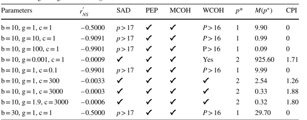
Table 1 Mitigation game: ΨM= −g <
0
For the general properties of the game (PEP, SAD, WCOH and MCOH), ✔ means that they hold for every coalition of size p . If this is not the case, p values indicated refer to intervals or specific values for which a given condition holds. For any other interval or values of p , the condition fails. If SAD holds for a given p , it means that the move from p −1 to p is superadditive. For h
�
(M) , Ψ, CPI , M(p
∗) and a(p∗) we round to two digits and for r′
NS we round to 4 digits
Parameters r′NS SAD PEP MCOH WCOH p* M(p∗) CPI
b = 10, g = 1, c = 1 – 0.5000 p > 17 ✔ ✔ P > 16 1 9.90 0 b = 10, g = 10, c = 1 – 0.9091 p > 17 ✔ ✔ P > 16 1 0.99 0 b = 10, g = 100, c = 1 – 0.9901 p > 17 ✔ ✔ P > 16 1 0.09 0 b = 10, g = 0.001, c = 1 – 0.0009 ✔ ✔ ✔ Yes 2 925.60 1.71 b = 10, g = 1, c = 0.1 – 0.9901 p > 17 ✔ ✔ P > 16 1 9.99 0 b = 10, g = 1, c = 300 – 0.0033 ✔ ✔ ✔ ✔ 2 2.54 1.26 b = 10, g = 1, c = 3000 – 0.0003 ✔ ✔ ✔ ✔ 2 0.33 1.88 b = 10, g = 1.9, c = 3000 – 0.0006 ✔ ✔ ✔ ✔ 2 0.32 1.80 b = 30, g = 1, c = 1 – 0.5000 p > 17 ✔ ✔ P > 16 1 29.70 0
12 The perhaps less interesting case of linear–quadratic payoff function could be easily obtained setting g=0.
Table 2 Effect of adap tation, firs t se t of simulations: Ψ M + A < 0 , h �(M ) >< 0 For the gener al pr oper ties of the game (PEP , S AD, W COH and MC OH), ✔ means that the y hold for ev er y coalition of size p . If this is no t t he case, p values indicated ref er t o inter vals or specific v alues f or whic h a giv en condition holds. F or an y o ther inter val or v alues of p , t he condition f ails. If S AD holds f or a giv en p , it means t hat t he mo ve fr om p − 1 to p is super additiv e. F or h � (M ) , Ψ , CPI , M (p ∗) and a (p ∗) w e r ound t o tw o digits and f or r ′ wNS e r ound t o 4 digits Par ame ters r ′ NS h � (M ) Ψ SA D PEP MC OH WC O H p* M (p ∗) a (p ∗) CPI M-Game: b = 10, g = 1, c = 1 – 0.5000 × – p > 17 ✔ ✔ P > 16 1 9.90 X 0 M + A
-Game: Effect of consider
ing adap tation β = 10, e = 1, f = 2, d = 5 – 0.4444 – 0.20 – 0.80 p > 17 ✔ ✔ p > 15 1 9.88 0.02 0 β = 10, e = 1, f = 1.5, d = 5 – 0.4872 – 0.10 – 0.95 p > 17 ✔ ✔ p > 15 1 9.37 1.06 0 β = 10, e = 1, f = 1.01, d = 5 – 0.4999 0 – 0.99 p > 17 ✔ ✔ p > 16 1 9.88 1.98 0 β = 10, e = 1, f = 2, d = 50 – 0.4949 – 0.02 – 0.98 p > 17 ✔ ✔ p > 15 1 9.89 0 0 β = 10, e = 1, f = 2, d = 1.000001 0 – 0.99 0 ✔ ✔ ✔ ✔ 2 0 9.99 0 β = 10, e = 2, f = 1, d = 5 – 0.4444 0.20 – 0.80 p > 17 ✔ ✔ p > 15 1 14.81 4.96 0 β = 10, e = 3, f = 1, d = 5 – 0.1666 0.40 – 0.20 p > 17 ✔ ✔ ✔ 1 66.66 28.66 0 β = 10, e = 1.01, f = 1, d = 5 – 0.4999 0 – 0.99 p > 17 ✔ ✔ p > 16 1 9.92 2.02 0 β = 10, e = 2, f = 1, d = 50 – 0.495 0.02 – 0.98 p > 17 ✔ ✔ p > 15 1 10.30 0.41 0 β = 10, e = 1, f = 2, d = 1.000001 0 0.99 0 ✔ ✔ ✔ ✔ 2 0 9.99 1.98
Table 3 Effect of adap tation, t hir d se t of simulations: Ψ M + A >< 0 , h �(M ) >< 0 * For the gener al pr oper ties of the game (PEP , S AD, W COH and MC OH), ✔ means that the y hold for ev er y coalition of size p . If this is no t t he case, p values indicated ref er t o inter vals or specific v alues f or whic h a giv en condition holds. F or an y o ther inter val or v alues of p , t he condition f ails. If S AD holds f or a giv en p , it means t hat t he mo ve fr om p − 1 to p is super additiv e. F or h � (M ) , Ψ , CPI , M (p ∗) and a (p ∗) w e r ound t o tw o digits and f or r ′ wNS e r ound t o 4 digits Simulations r ′ NS h � (M ) Ψ SA D PEP MC OH WC O H p* M (p ∗) a (p ∗) CPI M-Game: b = 10, g = 1, c = 3000 – 0.0003 × × ✔ ✔ ✔ ✔ 2 0.33 × 1.88 M + A
-Game: Effect of consider
ing adap tation β = 30, e = 1, f = 2.6, d = 5 – 0.0002 – 0.32 – 0.49 ✔ ✔ ✔ ✔ 2 0.01 6.00 0.0001 β = 30, e = 1, f = 1.1, d = 5 – 0.0003 – 0.02 – 0.99 ✔ ✔ ✔ ✔ 2 0.31 5.99 0.056 β = 30, e = 1, f = 2, d = 50 – 0.0032 – 0.02 – 0.98 ✔ ✔ ✔ ✔ 2 0.31 0.59 0.44 β = 30, e = 3.2, f = 1, d = 5 0 0.44 – 0.03 ✔ ✔ ✔ ✔ 2 0.78 6.34 0.33 β = 30, e = 1.1, f = 1, d = 5 – 0.0003 0.02 – 0.99 ✔ ✔ ✔ ✔ 2 0.35 6.01 0.07 β = 30, e = 2, f = 1, d = 50 – 0.0032 0.02 – 0.98 ✔ ✔ ✔ ✔ 2 0.35 0.61 0.53 β = 30, e = 1, f = 4.2, d = 10 0 – 0.32 0.02 ✔ ✔ ✔ ✔ 3 0.14 2.99 0.0006 β = 30, e = 1, f = 4.3, d = 10 0 – 0.33 0.09 ✔ ✔ ✔ ✔ 3 0.04 2.99 0.00004 β = 30, e = 1, f = 4.5, d = 12 0 – 0.29 0.02 ✔ ✔ ✔ ✔ 3 0.04 2.48 0.008 β = 30, e = 4.3, f = 1, d = 10 0 0.33 0.09 ✔ ✔ ✔ ✔ 3 0.69 3.22 1.31 β = 30, e = 4.6055, f = 1, d = 10 0.0001 0.36 0.29 ✔ ✔ ✔ ✔ 100 5.6 × 10 5 2.03 × 10 5 9.83 × 10 6 β = 30, e = 6, f = 1, d = 20 0.0001 0.25 0.25 ✔ ✔ ✔ ✔ 3 0.62 1.65 1.88 β = 30, e = 6.099, f = 1, d = 20 0.0001 0.25 0.29 ✔ ✔ ✔ ✔ 100 1.77 × 10 6 4.52 × 10 5 4.74 × 10 5
Table 4 Effect of adap tation, f our th se t of simulations: Ψ M + A > 0 , h �(M ) >< 0 * For the gener al pr oper ties of the game (PEP , S AD, W COH and MC OH), ✔ means that the y hold for ev er y coalition of size p . If this is no t t he case, p values indicated ref er t o inter vals or specific v alues f or whic h a giv en condition holds. F or an y o ther inter val or v alues of p , t he condition f ails. If S AD holds f or a giv en p , it means t hat t he mo ve fr om p − 1 to p is super additiv e. F or h � (M ) , Ψ , CPI , M (p ∗) and a (p ∗) w e r ound t o tw o digits and f or r ′ wNS e r ound t o 4 digits Simulations r ′ NS h � (M ) Ψ SA D PEP MC OH WC O H p* M (p ∗) a (p ∗) CPI M-Game: b = 10, g = 1.9, c = 3000 – 0.0006 x x ✔ ✔ ✔ ✔ 2 0.32 x 1.80 M + A
-Game: Effect of consider
ing adap tation β = 30, e = 1, f = 7.5, d = 20 0 – 0.33 0.21 ✔ ✔ ✔ ✔ 3 0.01 1.49 0 β = 30, e = 1, f = 7.5999, d = 19.8 0.0001 – 0.33 0.29 ✔ ✔ ✔ ✔ 100 2.27 0.76 0 β = 30, e = 7.5, f = 1, d = 20 0.0001 0.33 0.21 ✔ ✔ ✔ ✔ 3 0.70 1.72 2.19 β = 30, e = 7.5999, f = 1, d = 19.8 0.0001 – 0.33 0.29 ✔ ✔ ✔ ✔ 100 3X10 5 10 5 8.28 ×10 5
4.2.3 Simulation results
In our simulations, we extend the analysis of Bayramoglu et al. (2018) comparing the standard mitigation game with our new mitigation–adaptation game, analyz-ing the effects on stable coalition size, total mitigation and welfare. The followanalyz-ing results are highlighted:
Result 1 (climate cooperation in a pure mitigation setting, see Table 1)
In the mitigation game, our simulations confirm the analytical results of Bayra-moglu et al. (2018), as the two games do not differ. Stable coalitions can be formed at most by 2 players. In addition, we can qualify this result by showing that coopera-tion occurs when mitigacoopera-tion reaccoopera-tion funccoopera-tions are very flat. This can be intuitively explained by the fact that flat downward-sloping reaction functions produce less free riding incentives. Finally, we also find that the 2-player stable coalition brings just small welfare improvements compared to non-cooperation (small CPI), remaining far from the welfare improvements potentially achievable in full cooperation.
The addition of adaptation highlights different results depending on whether ΨM+A<0 or ΨM+A>0 , namely:
Result 2 (Effects of adaptation in case of ΨM+A<0 , see Tables 2 and 3)
With ΨM+A<0 , mitigation reaction functions remain downward sloping also in
the M + A-Game. Stable coalition size can be at most 2. This result is in line with Bayramoglu et al. (2018), which find that in case of downward-sloping reaction functions, the M + A-Game is not able to lead to larger stable coalitions. Nonethe-less, we find that, in some parameterization, the M-Game does not allow stable coa-lition to form, while the M + A-Game allows 2-player stable coacoa-litions. Hence, the introduction of adaptation can have a (small) positive influence on stable coalition size even when ΨM+A<0 . However, downward-sloping reaction functions still
pro-duce large free riding incentives, and larger stable coalitions are not possible. The M + A-Game generally leads to higher welfare equilibrium level than the M-Game. This happens because there are two instruments that can be used to cut climate change costs and, in a first best, two instruments can never perform worse than one. The gains are, however, small and the CPI index is always small. Finally, if the strategies are substitutes (complements), then the total mitigation level are lower (higher) in the M + A-Game than in the M-Game. The mitigation gap increases with the slope of the reaction function in the mitigation–adaptation space, i.e., h�(M) is
large in absolute terms.
Result 3 (Effects of adaptation in case of ΨM+A>0 , see Tables 3 and 4).
When ΨM+A>0 , the M + A-Game presents upward-sloping mitigation reaction
functions. In our configuration, ΨM+A>0 can be obtained only in those
parameteri-zations where in the M-Game reaction functions are extremely flat and the 2-player stable coalition forms. Upward-sloping reaction functions reduce the incentive to free ride: now, if signatories increase their mitigation levels, non-signatories will do the same. For this reason, larger stable coalitions are possible. Here our results differ from Bayramoglu et al. (2018). While they conclude that stable coalition size in the M + A-Game with upward-sloping reaction functions will be p∗ ≥3 , in our
p∗ = {3, n} . We find no other possible stable coalition size. This is in line with the
findings of Rubio (2019), which analyzes an emissions game with adaptation. Eventually, we can conclude that adaptation, when it leads to upward-sloping reaction functions, can make the grand coalition stable. Looking to the game proper-ties and Proposition 3, the enlargement of stable coalitions can be explained by more favorable condition for cooperation as, with upward-sloping mitigation reaction functions, superadditivity always holds. In turn, as MCOH always holds, WCOH follows.
When the stable coalition size is 3, total mitigation level in the stable coalitions is higher (lower) when adaptation and mitigation are complements (substitutes) com-pared to the M-Game. However, since coalition size is small, the welfare improve-ments are low (small CPI).
When the grand coalition forms, the social optimum is reached. Equilibrium miti-gation levels will always be higher in the M + A-Game than in the M-Game regard-less of the relationship between the two strategies. However, when mitigation and adaptation are substitute, the grand coalition only leads to small welfare improve-ments from non-cooperation. Conversely, if the social optimum is reached and the two strategies are complements, very high welfare improvements from the Nash equilibrium are achieved. We find this case, i.e., upward-sloping mitigation reac-tion funcreac-tions plus strategic complementarity between mitigareac-tion and adaptareac-tion, to be the only one to achieve both large participation and welfare improvements. However, as Proposition 1 shows, in our setting, upward-sloping mitigation reaction functions are less likely to be obtained compared to Bayramoglu et al. (2018). 5 Conclusion
This paper investigates how the presence of adaptation can influence the size and stability of international climate change agreements, their mitigation and welfare levels. It does so introducing a richer interaction across mitigation and adaptation. Namely, following the suggestions from the empirical and theoretical literature on adaptation, the possibility that adaptation effectiveness depends on the level of miti-gation is taken into account. In the light of this enrichment, the paper also re-exam-ines the nature of the strategic interaction between mitigation and adaptation.
Our analysis confirms that the presence of adaptation can make mitigation reac-tion funcreac-tions upward sloping. The interesting point is that this can occur when miti-gation and adaptation are either complement or substitute. What is needed is a “suf-ficiently large” interdependence across the two strategies. However, when adaptation effectiveness is made dependent upon mitigation levels, the possibility to observe this outcome reduces. Counterintuitive it may seem, this is explained by the fact that, with that modification, the positive externality produced by one’s mitigation on others increases: mitigation acts now not only reducing others’ climate change damages directly, but also indirectly, improving their adaptation effectiveness. This reinforces the tendency to reply with less mitigation by one player to more mitiga-tion by another player.
When mitigation reaction functions remain downward sloping, then the presence of adaptation does not enlarge the size of stable coalitions compared to the pure mit-igation game. However, there are more stable coalitions. When mitmit-igation reaction functions are upward sloping, adaptation increases the size of stable coalition In par-ticular, differently from Bayramoglu et al. (2018), we find that with upward-sloping reaction functions coalitions always form and they can be composed by either 3 or
n =100 players.
Complementarity or substitutability across mitigation and adaptation, on their turn, plays a crucial role in determining the abatement and the welfare level of the stable coalitions. With respect to this point, we show formally that complementarity can be originated when adaptation effectiveness depends upon mitigation levels.
When the two strategies are complements, for any given coalition size, individ-ual and total mitigation levels will be higher in the M + A-Game compared to the M-Game. If they are substitute, mitigation levels will be lower.
The M + A-Game generally leads to higher welfare equilibrium levels than the M-Game. This is intuitively because players are endowed with an additional instru-ment to maximize their objective function. With downward-sloping mitigation reac-tion funcreac-tions and small coalireac-tion size, the welfare gains are, however, small either compared to non-cooperation or the pure mitigation game. With upward-sloping mitigation reaction functions, in the cases in which the grand coalition forms, two situations can emerge. When there is mitigation–adaptation substitutability, the grand coalition is obtained only in cases where the need for cooperation is very low, i.e., the welfare improvement from non-cooperation is small. Instead, when we have mitigation–adaptation complementarity, when the grand coalition forms this will bring very high welfare improvement from non-cooperation.
We can derive two major policy implications from our work. The first is that a joint negotiation on mitigation and adaptation seems always welfare improving. Also when mitigation and adaptation are substitute, and mitigation reaction func-tions are downward sloping, adaptation increases the number of stable coalifunc-tions. This is a potentially positive message in the context of a fragmented regime or a bot-tom-up approach to climate negotiations like that endorsed by the Paris agreement. For instance, by supporting adaptation in developing countries, developed coun-tries could spur the formation of abating “clubs”, which could be a starting point to achieve further mitigation goals. Moreover if, as it seems possible, mitigation and adaptation are complements and mitigation reaction function are upward sloping, joint negotiation on mitigation and adaptation can lead to the formation of a sta-ble grand coalition. Here, however, we flag a second insight, which is less positive. Indeed, we showed that complementarity is facilitated when adaptation effectiveness is linked to mitigation level as suggested by many authors. Nonetheless, this same condition also shrinks the possibility to observe upward-sloping mitigation reaction functions, which is crucial for large abating coalitions. This suggests that also the “nature” of complementarity matters, and that in some cases, this can reduce the room for the formation of large and welfare improving mitigation coalition.
Possible extensions of this work could take into account, on the one hand, players heterogeneity, as considered, for instance, in Eyckmans et al. (2016) and Lazkano et al. (2016), and on the other hand, a more precise specification of the adaptation effectiveness function. In our explicit function, to satisfy the general assumptions and the non-negativity conditions, we considered adaptation effectiveness as a lin-early increasing function of total mitigation level. A more accurate representation could consider evidences from the literature to specify the concavity of this function. It could be also interesting to test our theoretical outcomes with an empirical appli-cation of an Integrated Assessment Model (IAM). IAMs have been already applied for coalition formation analysis in a pure mitigation context.13 However, despite
some models have been extended including adaptation (Agrawala et al. 2011; De Bruin et al 2009), coalition formation has not been analyzed.
Acknowledgement We would like to thank two anonymous reviewers for very helpful comments on a previous version of this paper.
Funding Open Access funding enabled and organized by Projekt DEAL.
Open Access This article is licensed under a Creative Commons Attribution 4.0 International License, which permits use, sharing, adaptation, distribution and reproduction in any medium or format, as long as you give appropriate credit to the original author(s) and the source, provide a link to the Creative Com-mons licence, and indicate if changes were made. The images or other third party material in this article are included in the article’s Creative Commons licence, unless indicated otherwise in a credit line to the material. If material is not included in the article’s Creative Commons licence and your intended use is not permitted by statutory regulation or exceeds the permitted use, you will need to obtain permission directly from the copyright holder. To view a copy of this licence, visit http://creat iveco mmons .org/licen ses/by/4.0/.
Appendix
Proof of Lemma 1, Additional Assumption, and Proposition 1
Proof of Lemma 1 is obtained through the comparison of signatories and non-sig-natories FOCs in mitigation space. Details of the proof are available in the Online Appendix.
For what concerns the derivation of the existence and uniqueness condition, we only consider the M + A-Game as we know from Bayramoglu et al. (2018) that existence and uniqueness are always guaranteed in the M-Game. The procedure fol-lows Bayramoglu et al. (2018) and it is reported in the Online Appendix.
Finally, mitigation FOCs (4a) and (4b) in the M-Game and (5a) and (5b) in the M + A-Game implicitly define individual reaction functions in mitigation space for signatories and non-signatories, respectively. Slopes of individual reaction functions are obtained through differentiations of these FOCs. The detailed derivation is avail-able in the Online Appendix.
Proof of Proposition 2 and Corollary
In the M + A-Game, considering the first-order condition (6), we can characterize the optimal adaptation level a∗ , equal for both signatories and non-signatories, as a
function of total mitigation M. We can rewrite the FOC for adaptation as:
This FOC expresses the reaction function in the mitigation–adaptation space
h(M) . Differentiating it with respect to M and readjusting, we obtain the slope of this
function:
From the general assumptions, the denominator is positive and therefore, the sign of this equation depends on the numerator. The first term of BaM is negative, while
the second term is positive. We have strategic substitutability (complementarity) between mitigation and adaptation if BaM+ Ba𝜀⋅ 𝜀M<(>)0.
Corollary We want to analyze the effect of introducing adaptation on total miti-gation level. Looking to M + A-Game mitimiti-gation FOCs (5a) and (5b), we see that
adaptation has a double effect on them: first, it reduces BM as BMa<0 and, second,
it increases B𝜀 as B𝜀a>0 . Depending on which of these two effects dominates the
other, we can have higher or lower individual mitigation levels in the M + A-game than in the M-game. If the adaptation effect on the left-hand side of Eqs. (5a) and (5b) is positive, then mitigation levels will increase as the cost function is convex,
while the benefit function is concave. Vice versa, mitigation levels will decrease. The M + A-Game mitigation levels, both for signatories and non-signatories, will be higher than M-game mitigation levels if BMa+ B𝜀a⋅ 𝜀M>0 . This condition,
look-ing to the general assumptions of the model, is equal to BaM which also determines
the sign of h�(M) . Therefore, we will have higher (lower) mitigation levels in the
M + A-game respect to the M-Game if adaptation and mitigation are strategic com-plements (substitutes). Comparing this with the results of Bayramoglu et al. (2018),
we can see the difference effect of the introduction of adaptation under the standard assumption of substitutability. The second relation between mitigation and adapta-tion that we insert reduces (or invert) the strategic substitutability of the two strate-gies. It follows that the introduction of adaptation in our model leads to a lower decrease of mitigation levels compared with Bayramoglu et al. (2018).
Ba(M, a∗(M), 𝜀(M)) = Da(a ∗ (M)). h�(M) =𝜕a ∗ 𝜕M = BaM+ Ba𝜀⋅ 𝜀M Daa− Baa = BaM Daa− Baa .
Proof of Proposition 3
For the M-Game, the conclusions on superadditivity, PEP and MCOH have already been proved by Bayramoglu et al. (2018). We focus instead on our M + A-Game version. The proofs follow the same procedure of Bayramoglu et al. (2018) and are available in the Online Appendix.
Preliminaries of explicit payoff functions
For the explicit payoff function of the pure mitigation game, all the assumptions of the model and the existence and uniqueness condition are always satisfied irrespec-tive of the (posiirrespec-tive) parameters values as in Bayramoglu et al. (2018)14, 15
Moving to the M + A-Game, we look to the explicit payoff function (8). Doing some simple partial derivatives, we look to the correspondence between the prop-erty of this function and the general assumptions:
Adaptation–mitigation strategic interaction
From ΨM+A= B MM+ ( BaM) 2 Daa−Baa we get Ψ M+A= −g +(e−f )2 d = (e−f )2−g⋅d d . The sign of
ΨM+A depends on the difference (e − f )2− g ⋅ d . The additional assumption on
exist-ence and uniqueness condition is: ΨM+A
⋅ [ p2 Cmm(mS) + (n−p) Cmm(mNS) ]
<1 . For our explicit payoff function, the condition is most restrictive when p = n and therefore we
BM= BM+ B𝜀⋅ 𝜀M= b − g ⋅ M + (e − f ) ⋅ a, BMM= −g < 0, Cm= c ⋅ mi>0, Cmm= c > 0. Ba= 𝛽 + (e − f ) ⋅ M, Baa= 0, Da= d ⋅ a > 0, Daa= d > 0. 𝜀M= e > 0, 𝜀MM= 0. B𝜀= a > 0, B𝜀𝜀= 0, B𝜀M= B𝜀𝜀⋅ 𝜀M= 0. BaM= −f < 0. Ba𝜀= 1. BaM= BaM+ Ba𝜀⋅ 𝜀M= −f + e. 14 B
aM indicates the mitigation–adaptation cross derivative without considering the effects on
adapta-tion effectiveness, i.e., BaM is computed from the welfare function (8) ignoring the effectiveness function 𝜀(M) = e ⋅ M.
15 B
aM indicates the overall adaptation–mitigation cross derivative. It takes into account the standard
negative effect (BaM= −f
) and the positive effect (B
a𝜀⋅ 𝜀M= e
) that mitigation has on adaptation mar-ginal benefits through the effectiveness function 𝜀(M) = e ⋅ M.
obtain: ΨM+A
⋅n2
Cmm(ms) <1 and, substituting the values and rearranging:
c ⋅ d − n2
⋅(g⋅ d − (e − f )2) > 0. For reaction functions, we derive.
in mitigation space and
in mitigation–adaptation space.
Reaction functions in the mitigation space will be downward (upward) sloping if ΨM+A= (e−f )2−g⋅d
d <(>)0 . Reaction functions in the mitigation–adaptation space
will be downward (upward) sloping if BaM = e − f < (>)0 , i.e., mitigation and
adap-tation will be strategic substitutes (complements) if e − f < (>)0.
Looking to mitigation and adaptation levels, we obtain:
mS= p⋅c⋅d⋅(b⋅d+𝛽⋅(e−f )) (p2+n−p) ⋅(d⋅g−(e−f )2)+c⋅d , mNS= c⋅d⋅(b⋅d+𝛽⋅(e−f )) (p2+n−p) ⋅(d⋅g−(e−f )2)+c⋅d and a = (p 2+n−p) ⋅(b⋅(e−f )+𝛽⋅)g+𝛽⋅c (p2+n−p) ⋅(d⋅g−(e−f )2)+c⋅d.
The denominator of mitigation and adaptation levels is always positive because of the existence and uniqueness condition. Hence, the following conditions need to be satisfied in the parameters’ choice for the M + A-Game simulations:16
where C1 and C2 are required for the general assumptions to hold, C3 is the most restrictive existence and uniqueness condition, C4 and C5 are, respectively, the miti-gation and adaptation non-negativity conditions.
r�S(M−i) = p ⋅((e − f )2− d ⋅ g) c ⋅ d − p ⋅((e − f )2 − d ⋅ g) and r � NS(M−j) = (e − f )2− d ⋅ g d ⋅ g − (e − f )2+ c ⋅ d, h�(M) = e − f d , C1 ∶ b − g ⋅ M + (e − f ) ⋅ a > 0, C2 ∶ 𝛽 + (e − f ) ⋅ M > 0, C3 ∶ c ⋅ d − n2⋅(g⋅ d − (e − f )2) > 0, C4 ∶ b ⋅ d + 𝛽 ⋅ (e − f ) > 0, C5 ∶(p2+ n − p)⋅ (b ⋅ (e − f ) + 𝛽⋅)g + 𝛽 ⋅ c > 0,
16 C1 and C2 are required to have B