UNIVERSITÀ DEGLI STUDI DI SASSARI CORSO DI DOTTORATO DI RICERCA
Scienze Agrarie
Curriculum Agrometeorologia ed Ecofisiologia dei Sistemi Agrari e Forestali Ciclo XXX
Coupling remote sensing with wildfire spread modeling in
Mediterranean areas
Olga Muñoz Lozano
Coordinatore del Corso
Prof. Ignazio Floris
Referente di Curriculum
Prof. Maurizio Mulas
Docente Guida
Docente Tutor
Prof. Donatella Spano
Dr. Michele Salis
Index
List of abbreviations 1
Abstract 3
Introduction 5
Chapter 1 13
Mapping fuel types combining Multispectral and LiDAR data of Sardinia Chapter 2 45
Characterizing Mediterranean Canopy fuel properties from LiDAR data Chapter 3 71
Integrating LiDAR and satellite data with wildfire spread modeling to enhance wildfire exposure analysis in Mediterranean areas Final conclusions 90
Acknowledgements 93
Appendices 95
Appendix A 97
Maps obtained from the classification outputs carried out with the different algorithms and in the study area of Siniscola. Appendix B 103
Maps obtained from the classification outputs carried out with the different algorithms and in the study area of Muravera. Appendix C 109
Confusion matrices from the classifications carried out with the different algorithms for the study area of Siniscola. Appendix D 117
Confusion matrices from the classifications carried out with the different algorithms for the study area of Muravera. Appendix E 125
List of Abbreviations
AAD Absolute Average Deviation
AGEA AGenzia per le Erogazioni in Agricoltura (Agricultural Supplies Agency)
AIC Akaike Information Criteria
ASCII American Standard Code for Information Interchange
CBD Canopy Bulk Density
CBH Canopy Base Height
CFR Crown Fire Activity
CUS Custom
CV Coefficient of Variation DBH diameter at breast height DEM Digital Elevation Model
EEA European Environmental Agency
Elev Elevation
FLI Fireline Intensity
FMC dead fuel moisture content
FML Flame Length
H1, H2 and H3 first, second and third strata of mean height respectively
HPA Heat per unit Area
IQ InterQuartile
K Cohen’s Kappa coefficient
LCP Landscape file
LiDAR Light Detection And Ranging
LMM Linear Mixed Models
LUM Land Use Map
MAD Median of the Absolute Deviations
MTT Minimum Travel Time
NDII Normalized Difference Infrared Index NDVI Normalized Difference Vegetation Index
NIR Near InfraRed
NN Neural Networks
OA Overall Accuracy
RCI Reaction Intensity
RF Random Forests
ROS Rate of Spread
SAVI Soil Adjusted Vegetation Index SC Sørensen’s coeffcient
SD1, SD2 and SD3
first, second and third strata of standard deviation respectively
SDR Spread Direction
SH Stand Height
ST Standard
SVM Support Vector Machine
SWIR Short Wave InfraRed
TOA Time of Arrival
UTM Universal Transverse of Mercator WGS-84 World Geodetic System 1984
Abstract
Wildfires are a threat to the ecosystems and in the future this threat could become stronger due to climate change. Spatially explicit fire spread models are effective tools to study fire behavior and wildfire risk. However, to run fire spread simulations, one of the most important inputs is represented by fuel models and this information is not always available. In the last decades, remote sensing technologies have offered valuable information for the classification and characterization of fuels. For this reason, in this work we created accurate maps of main fuel types for Mediterranean areas combining multispectral and LiDAR data. This information improves the current available information, which derives from the Land Use Map of Sardinia. We also enhanced the characterization of canopy fuel models using LiDAR data producing canopy layers ready to be used for wildfire spread modeling. Finally, we compared the variation in simulated wildfire spread and behavior determined by the use of fine-scale maps v. lower resolution maps. In these simulations, we assessed also the effect of using LiDAR-derived canopy layers as well. The results showed more accurate outputs when using our custom fuel and canopy layers produced in this work. In conclusion, this work suggests that the use of LiDAR and satellite imagery data can contribute to improve estimates of modeled wildfire behavior.
Introduction
Wildfires threat ecosystems worldwide (Cole and Landres 1996; Pausas and Keeley 2009) and especially in Mediterranean areas (Syphard et al. 2009). For instance, in 2016 in Europe the 68% of fires occurred in Mediterranean countries and these fires accounted for 93% of the overall burned area of Europe (San-Miguel-Ayanz et al. 2017).
In the future, wildfires impacts on ecosystems are expected to increase due to climate change (mainly higher temperatures and more frequent heat waves, Flannigan et al. 2000, 2009; Liu et al. 2010; Arca et al. 2012; Kovats et al. 2014; Kurnik et al. 2017; Lozano et al. 2017). Studies carried out to investigate the effects of recent warming on wildfire season length and behavior confirmed that higher temperatures bring with them prolonged fire seasons and longer fire events, as well as more fire ignitions and larger fires (Piñol et al. 1998; Westerling et al. 2006; Turco et al. 2014; Urrutia-Jalabert et al. 2018). Indeed, (Kovats et al. 2014) predicted warmer and drier weather (especially in summer) with increased fire risk in Mediterranean areas.
In a context of likely increase of wildfire-derived damages (particularly from large fires, which account for the most of burned area although limited in number), the advances in fire behavior analysis and in the assessment of fire risk will play a key role for fire management and research.
A number of papers reported that spatially explicit fire spread models are effective tools to study wildfire behavior and risk (e.g.: Calkin et al. 2011; Miller and Ager 2013). Most of fire spread models are based on physical principles and empirical observations (Duff et al. 2013). The use of fire simulators was proved to be an effective and powerful tool not only for Northern America ecosystems, (Thompson et al. 2011; Ager et al. 2013, 2014) but also in the Mediterranean area (Salis et al. 2014; Alcasena et al. 2015; Kalabokidis et al. 2015).
To run fire spread simulations, one of the most important inputs is represented by fuel distribution. The spread of fire is affected for some fuel factors such as crown bulk density, crown base height, canopy height, percent of canopy cover, surface
area-to-volume ratio, vertical and horizontal continuity, dead and live fuel load, and size classes of fuel elements (Riaño et al. 2003). For that reason, the vegetation is operationally classified into different fuel types following a scheme of fuel properties that groups the vegetation classes with similar combustion behavior (Pyne et al. 1996). The accuracy of the fuel map used as input in fire spread simulations highly affects the results obtained. Moreover, the consistency and accuracy of the input data layers are very important for realistic predictions of fire growth (Finney 1998; Keane et al. 1998).
Traditionally, fuel types have been mapped by means of aerial photography and extensive fieldwork, which is highly expensive and time consuming (Riaño et al. 2003; Arroyo et al. 2008; Marino et al. 2016). Remote sensing data provide an alternative as source of fuel information, since they can provide spatial information on land cover. Fuel type mapping from satellite imagery has been attempted by several authors (Lasaponara and Lanorte 2007a; b; Mallinis et al. 2008; Otukei and Blaschke 2010). However, the main limitation of satellite images is their inability to estimate heights and to estimate vertical distribution of forest stands (Arroyo et al. 2008). These factors are critical not only for fuel type discrimination, but also for assessing some fuel characteristics needed for fire spread modeling such as fuel load, canopy cover, tree height, crown base height, and crown bulk density (Riaño et al. 2003). Light Detection And Ranging (LIDAR) allows overcoming these limitations (Arroyo et al. 2008). The ability of penetrating the canopy layer is leading authors to include LiDAR data as an essential source of information for fuel types mapping and fuel characterization (Riaño
et al. 2003; Mutlu et al. 2008; Erdody and Moskal 2010; García et al. 2011;
González-Ferreiro et al. 2014; Hermosilla et al. 2014; Marino et al. 2016; Ruiz et al. 2018).
In this context, the aims of the following three chapters are 1) to create accurate maps of main fuel types for Mediterranean areas combining multispectral and LiDAR data; 2) to improve the characterization of canopy fuel models using LiDAR data; and 3) to compare the variation in simulated wildfire spread and behavior determined by the use of fine-scale v. lower resolution maps, and to assess the effect of using our custom canopy layers in the simulations. The final objective is to develop a methodology for creating those maps and canopy layers which could
REFERENCES
Ager AA, Buonopane M, Reger A, Finney MA (2013) Wildfire Exposure Analysis on the National Forests in the Pacific Northwest, USA. Risk Analysis 33, 1000–1020. doi:10.1111/j.1539-6924.2012.01911.x.
Ager AA, Day MA, McHugh CW, Short K, Gilbertson-Day J, Finney MA, Calkin DE (2014) Wildfire exposure and fuel management on western US national forests. Journal of Environmental Management 145, 54–70. doi:10.1016/j.jenvman.2014.05.035.
Alcasena FJ, Salis M, Ager AA, Arca B, Molina D, Spano D (2015) Assessing Landscape Scale Wildfire Exposure for Highly Valued Resources in a Mediterranean Area. Environmental Management 55, 1200–1216. doi:10.1007/s00267-015-0448-6.
Arca B, Pellizzaro G, Duce P, Salis M, Bacciu V, Spano D, Ager AA, Scoccimarro E (2012) Potential changes in fire probability and severity under climate change scenarios in mediterranean areas. In: Spano D, Bacciu V, Salis M, Sirca C (eds) ‘International Conference on Fire Behaviour and Risk’, Alghero (Italy). 92–98.
Arroyo LA, Pascual C, Manzanera A (2008) Fire models and methods to map fuel types: The role of remote sensing. Forest Ecology and Management 256, 1239– 1252. doi:10.1016/j.foreco.2008.06.048.
Calkin DE, Thompson MP, Finney MA, Hyde KD (2011) A real-time risk assessment tool supporting wildland fire decision-making. Journal of Forestry 109, 274–280.
Cole DN, Landres PB (1996) Threats to wilderness ecosystems: impacts and research needs. Ecological Applications 6, 168–184. doi:10.2307/2269562.
Duff TJ, Chong DM, Tolhurst KG (2013) Quantifying spatio-temporal differences between fire shapes: Estimating fire travel paths for the improvement of dynamic spread models. Environmental Modelling & Software 46, 33–43. doi:10.1016/j.envsoft.2013.02.005.
Erdody TL, Moskal LM (2010) Fusion of LiDAR and imagery for estimating forest canopy fuels. Remote Sensing of Environment 114, 725–737. doi:10.1016/j.rse.2009.11.002.
Finney MA (1998) FARSITE : Fire Area Simulator — Model Development and Evaluation. USDA Forest Service, Rocky Mountain Research Station, RMRS-RP-4. (Ogden, UT) http://www.firemodels.org/content/view/52/72/.
Flannigan MD, Krawchuk M a, de Groot WJ, Wotton BM, Gowman LM (2009) Implications of changing climate for global wildland fire. International Journal of
Wildland Fire 18, 483–507. doi:10.1071/WF08187.
Flannigan MD, Stocks BJ, Wotton BM (2000) Climate change and forest fires. Science
of The Total Environment 262, 221–229. doi:10.1016/S0048-9697(00)00524-6.
García M, Riaño D, Chuvieco E, Salas J, Danson FM (2011) Multispectral and LiDAR data fusion for fuel type mapping using Support Vector Machine and decision rules. Remote Sensing of Environment 115, 1369–1379. doi:10.1016/j.rse.2011.01.017.
González-Ferreiro E, Diéguez-Aranda U, Crecente-Campo F, Barreiro-Fernández L, Miranda D, Castedo-dorado F (2014) Modelling canopy fuel variables for Pinus radiata D . Don in NW Spain with low-density LiDAR data. 23, 350–362. doi:10.1071/WF13054.
Hermosilla T, Ruiz LA, Kazakova A, Coops NC, Moskal LM (2014) Estimation of forest structure and canopy fuel parameters from small-footprint full-waveform LiDAR data. International Journal of Wildland Fire 23, 224–233.
doi:10.1071/WF13086.
Kalabokidis K, Palaiologou P, Gerasopoulos E, Giannakopoulos C, Kostopoulou E, Zerefos C (2015) Effect of Climate Change Projections on Forest Fire Behavior and Values-at-Risk in Southwestern Greece. Forests 6, 2214–2240. doi:10.3390/f6062214.
Keane RE, Garner JL, Schmidt KM, Menakis JP, Finney MA (1998) Development of input data layers for the FARSITE fire growth model for the Selway-Bitterroot Wilderness Complex, USA. USDA Forest Service, Rocky Mountain Research Station, RMRS-GTR-3. (Fort Collins, CO)
Kovats S, Valentini R, Bouwer LM, Georgopoulou E, Jacob D, Martin E, Rounsevell M, Soussana J-F (2014) Chapter 23. Europe. In: Barros et al. (eds) Climate Change 2014: Impacts, Adaptation and Vulnerability Contribution of Working Group II to the Fifth Assessment Report of the Intergovernmental Panel on Climate Change. Cambridge University Press, (Cambridge) doi:10.1017/CBO9781107415324.004.
Kurnik B, Van Der Linden P, Mysiak J, Swart R, Füssel H-M, Christiansen T, Cavicchia L, Gualdi S, Mercogliano P, Rianna G, Kramer K, Michetti M, Salis M, Schelhaas M-J, Leitner M, Vanneuville W, Macadam I (2017) Chapter 3. Weather- and climate-related natural hazards in Europe. In: Climate change adaptation and disaster risk reduction in Europe - Enhancing coherence of the knowledge base, policies and practices. Publications Office of the European Union, (Luxembourg) doi:10.2800/938195.
Lasaponara R, Lanorte A (2007a) Remotely sensed characterization of forest fuel types by using satellite ASTER data. International Journal of Applied Earth Observation
and Geoinformation 9, 225–234. doi:10.1016/j.jag.2006.08.001.
Lasaponara R, Lanorte A (2007b) On the capability of satellite VHR QuickBird data for fuel type characterization in fragmented landscape. Ecological Modelling 204, 79– 84. doi:10.1016/j.ecolmodel.2006.12.022.
Liu Y, Stanturf J, Goodrick S (2010) Trends in global wildfire potential in a changing climate. Forest Ecology and Management 259, 685–697. doi:10.1016/j.foreco.2009.09.002.
Lozano OM, Salis M, Ager AA, Arca B, Alcasena FJ, Monteiro AT, Finney MA, Giudice L Del, Scoccimarro E, Spano D (2017) Assessing Climate Change Impacts on Wildfire Exposure in Mediterranean Areas. Risk Analysis 37, 1799–2022. doi:10.1111/risa.12739.
Mallinis G, Mitsopoulos ΙD, Dimitrakopoulos AP, Gitas IZ, Karteris M (2008) Local-Scale Fuel-Type Mapping and Fire Behavior Prediction by Employing High-Resolution Satellite Imagery. IEEE Journal of Selected
Topics in Applied Earth Observations and Remote Sensing 1, 230–239.
doi:10.1109/JSTARS.2008.2011298.
Marino E, Ranz P, Luis J, Ángel M, Esteban J, Madrigal J (2016) Remote Sensing of Environment Generation of high-resolution fuel model maps from discrete airborne laser scanner and Landsat-8 OLI : A low-cost and highly updated methodology for large areas. Remote Sensing of Environment 187, 267–280. doi:10.1016/j.rse.2016.10.020.
Miller C, Ager AA (2013) A review of recent advances in risk analysis for wildfire management. International Journal of Wildland Fire 22, 1–14. doi:10.1071/WF11114.
Mutlu M, Popescu SC, Stripling C, Spencer T (2008) Mapping surface fuel models using lidar and multispectral data fusion for fire behavior. 112, 274–285. doi:10.1016/j.rse.2007.05.005.
Otukei JR, Blaschke T (2010) Land cover change assessment using decision trees, support vector machines and maximum likelihood classification algorithms.
International Journal of Applied Earth Observation and Geoinformation 12, 27–
31. doi:10.1016/j.jag.2009.11.002.
Pausas JG, Keeley JE (2009) A Burning Story: The Role of Fire in the History of Life.
BioScience 59, 593–601. doi:10.1525/bio.2009.59.7.10.
Piñol J, Terradas J, Lloret F (1998) Climate warming, wildfire hazard, and wildfire occurrence in coastal eastern Spain. Climatic Change 38, 345–357. doi:10.1023/A:1005316632105.
Pyne SJ, Andrews PL, Laven RD (1996) ‘Introduction to wildland fire.’ (John Wiley and Sons: New York)
Riaño D, Meier E, Allgöwer B, Chuvieco E, Ustin SL (2003) Modeling airborne laser scanning data for the spatial generation of critical forest parameters in fire behavior modeling. Remote Sensing of Environment 86, 177–186. doi:10.1016/S0034-4257(03)00098-1.
Ruiz LÁ, Recio JA, Crespo-Peremarch P, Sapena M (2018) An object-based
approach for mapping forest structural types based on low density LiDAR and multispectral imagery. Geocarto International 33, 443–457.
doi:10.1080/10106049.2016.1265595.
Salis M, Ager AA, Finney MA, Arca B, Spano D (2014) Analyzing spatiotemporal changes in wildfire regime and exposure across a Mediterranean fire-prone area.
Natural Hazards 71, 1389–1418. doi:10.1007/s11069-013-0951-0.
San-Miguel-Ayanz J, Durrant T, Boca R, Libertà G, Branco A, De Rigo D, Ferrari D, Maianti P, Artés Vivancos T, Schulte E, Loffler P (2017) Forest Fires in Europe, Middle East and North Africa 2016. Publications Office of the European Union, doi:10.2760/17690.
Syphard AD, Radeloff VC, Hawbaker TJ, Stewart SI (2009) Conservation Threats Due to Human-Caused Increases in Fire Frequency in Mediterranean-Climate Ecosystems. Conservation Biology 23, 758–769. doi:10.1111/j.1523-1739.2009.01223.x.
Thompson MP, Calkin DE, Finney MA, Ager AA, Gilbertson-Day JW (2011) Integrated national-scale assessment of wildfire risk to human and ecological values. Stochastic Environmental Research and Risk Assessment 25, 761–780.
Turco M, Llasat M-C, von Hardenberg J, Provenzale A (2014) Climate change impacts on wildfires in a Mediterranean environment. Climatic Change 125, 369–380. doi:10.1007/s10584-014-1183-3.
Urrutia-Jalabert R, González ME, González-Reyes Á, Lara A, Garreaud R (2018) Climate variability and forest fires in central and south-central Chile. Ecosphere 9,. doi:10.1002/ecs2.2171.
Westerling AL, Hidalgo HG, Cayan DR, Swetnam TW (2006) Warming and Earlier Spring Increase Western U.S. Forest Wildfire Activity. Science 313, 940–943. doi:10.1126/science.1128834.
Chapter 1: Mapping fuel types combining
Multispectral and LiDAR data of Sardinia
1. INTRODUCTION
Accurate fuel maps are not only a critical input for fire spread models, but also to plan fire prevention, management and suppression activities. The availability of accurate and spatially explicit information on fuel properties is critical in order to improve fire management decision-support systems since fuels affect fire ignition and propagation (Ottmar and Alvarado 2004; Chuvieco et al. 2009).
The high spatial and temporal variability of fuels makes field survey methods very expensive and time consuming for obtaining realistic characterization, and often limited for fuel mapping. Hence methods based on aerial photography and remotely sensed data have risen in the last years (Arroyo et al. 2008; Bajocco et al. 2015). Most studies based on satellite imagery have been performed at a coarse resolution or in very small areas with a very high resolution (Lasaponara and Lanorte 2007a; b, Mallinis et al. 2008, 2014; Otukei and Blaschke 2010).
As far as LiDAR (Light Detection and Ranging) is concerned, though these data have proved to be suitable to estimate some fuel properties, few studies have evaluated their usefulness to create fuel maps because of the difficulties in identifying land cover classes only from this data source (Yan et al. 2015).
The most important limitation of optical images is their inability to assess vegetation height, which is a critical variable to discriminate fuel types. The integration of LiDAR data allows overcoming this limitation (Arroyo et al. 2008).
In the last years some works have combined LiDAR and satellite imagery to map fuels, but the identification of individual species stills remain a complex task. Varga and Asner (2008) developed a new fire fuel index through the fusion of hyperspectral and LiDAR data to model the three-dimensional volume of grass fuels. Koetz et al. (2008) used LiDAR and hyperspectral data to map different land cover types including roads, buildings and vegetation but with only three vegetation types (ground fuel, shrubs and
tree canopy). Also García et al. (2011) combined LiDAR and multispectral data in this case, for fuel mapping, but since they followed the Prometheus fuel type system to classify the different fuel types, only structural characteristics were considered such as the average height of vegetation or the average height difference between shrubs and trees. Recently, Reese et al. (2014) classified alpine vegetation combining optical satellite data and LiDAR derived data, and Marino et al. (2016) obtained fuel model maps from discrete airborne laser scanner and Landsat-8 OLI (30-m resolution).
Regarding Sardinia, there are no fuel type maps for the whole island at fine scale. Until now, the maps used to derive fuel type information are coarse resolution land use maps (e.g. Corine Land Cover, EEA 2011 or Land Use Map of Sardinia, Autonomous Region of Sardinia 2008).
The overall aim of the work is to improve the available information about the fuel types spatial distribution by creating accurate fuel maps at fine scale from remotely sensed data, namely combining LiDAR with multispectral data.
2. METHODS
2.1. Study area
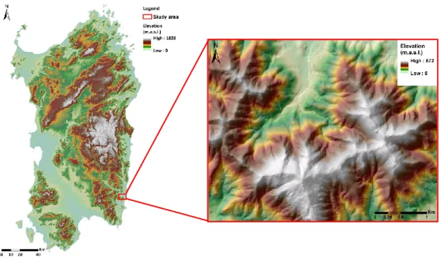
The study is performed in the island of Sardinia (Italy), which is located between 38° 44‟ and 41° 05‟ N latitude and 8° 7‟ and 9° 49‟ E longitude. The availability of LiDAR data for the island is limited to the coastal areas and, within these boundaries, two study areas covering approximately the same extent (4,000 ha approximately) were selected to carry out this work (Fig. 1.1). These areas are located on the eastern coast (Siniscola)
and were selected to include in the study different types of vegetation structures that can be often found in Sardinia (i.e.: broadleaf forests and Mediterranean maquis).
2.2. Classification method
Fig. 1.2. Work flow diagram showing the main steps for producing a fuel map. DEM = Digital Elevation Model
The fuel type classification was carried out following the scheme showed in figure 1.2. After processing remote sensing data (see sections 2.4 and 2.5), we obtained a series of layers with a number of variables (bands of multispectral data, spectral indices and height distribution statistics and canopy cover from LiDAR). Then a set of reference areas was defined to determine their actual land cover type. For this analysis, we used as source of reference data, an orthophoto co-registered with simultaneously acquired LiDAR data (0.1m-resolution).
The calibration and validation of the classification model has been done by assigning the corresponding LiDAR-derived metrics and Spot-5 reflectance values to the reference areas (where the fuel type is already known). We used 70% of reference areas to fit the model and 30% to validate it.
We evaluated four different algorithms which are commonly used to classify remote sensed data: Maximum Likelihood (ML), Neural Networks (NN), Support Vector
Machine (SVM) and Random Forests (RF).
The maximum likelihood (ML) algorithm is one of the most widespread parametric methods that have been traditionally used for classification of remote sensing data (Martin et al. 1998; Walter 2004; Shalaby and Tateishi 2007). Since a normal distribution within each class is assumed, a probability function of a pixel belonging to a certain class can be calculated according to the training data‟s values. In this way, the ML classifier assigns the pixel to the class which maximizes the probability function (Chuvieco 2010).
However, since parametric methods implies assumptions such as the normal distribution of data, alternative non-parametric methods like artificial neural networks (NN) have been employed to classify remote sensing images(Frizzelle and Moody 2001; Qiu and Jensen 2004; Yuan et al. 2009). Neural networks are able to learn from training data creating a complex classification scheme which is used to classify the rest of observations (Chuvieco 2010). They try to mimic the neural storage and analytical operations of the brain where “neurons” are interconnected through weighted relationships (Frizzelle and Moody 2001).
Another non-parametric method used in remote sensing classification is suppport
vector machine (SVM) which is also a machine learning algorithm (Pal and Mather
2005; García et al. 2011; Mountrakis et al. 2011). Using the training data, the algorithm attempts to find a hyperplane that separates the dataset into a discrete predefined classes minimizing misclassifications (Mountrakis et al. 2011).
Recently random forests (RF) have been also introduced for remote sensed data analysis, especially for LiDAR data (Falkowski et al. 2009; Yu et al. 2011; Valbuena et
al. 2016), but it has been also used for classifying optical data (Pal 2005; Reese et al.
2014). It is a non-parametric method which consists of a combination of decision trees classifiers where different samples are randomly chosen from the training data to construct each individual tree (Breiman 2001). This algorithm searches only a random subset of the variables in order to minimize the correlation between the classifiers in the ensemble.
These different classification were carried out using the R package „Rasclass‟ (R Core Team 2016; Wiesmann and Quinn 2016). Finally we built four fuel maps for each study area following the different classification model obtained from the outputs of each algorithm.
2.3. Fuel types
In this work, the fuel types that we discriminated with the proposed methodology are those shown in table 1.1. We selected these fuel types because they have been already characterized and/or tested in other studies in Sardinia (Arca et al. 2007, 2009, Salis et
al. 2013, 2016, 2018; Ager et al. 2014; Alcasena et al. 2015). To compare our outputs
with the information available until now, we also reclassified the Land Use Map (LUM) of Sardinia (Autonomous Region of Sardinia 2008) for the same fuel types. The original classes of the LUM of Sardinia are based on the Corine Land Cover classification (EEA 2011). The LUM of Sardinia was elaborated using different sources such as: ortophoto AGEA (AGenzia per le Erogazioni in Agricoltura) 2003, ortophoto 2004, images Ikonos 2005-06, images Landsat 2003 and images Aster 2004. As reference data, 4000 sample site were set throughout the island.
Table 1.1. Fuel types to be mapped and corresponding classes of the Land Use Map (LUM) of sardinia.
Code Fuel type LUM Classes
1 Buildings (non-fuel) 143, 1111, 1112, 1121, 1122, 1211, 1212, 1224, 1421 2 Roads (non-fuel) 123, 1221, 1322, 1421 3 Water 3315, 5111, 5112, 5122, 5211, 5212, 5231 4 Bare ground 131, 133, 1321, 3311 5 Sparse vegetation 333, 3313 6 Mixed agricultural 242, 243, 2112, 2121, 2123 7 Vineyard and orchard 221, 222, 223, 2411, 2413 8 Herbaceous vegetation 321, 2111 9 Garrigue 244, 411, 421, 3232, 3241 10 Mediterranean maquis 3221, 3222, 3231 11 Conifer forests 313, 3121, 3242 12 Broadleaf forests 3111, 31121, 31122 13 Mixed forests 141, 313
2.4. LiDAR data processing
LiDAR data of the study area in ASCII (.xyz) format were provided by the Autonomous Region of Sardinia (Servizio osservatorio del paesaggio e del territorio, sistemi informativi territoriali). These LiDAR data were recorded in different periods from 21st October 2008 to 10th May 2009 using as laser equipment an Altm GEMINI sensor and obtaining a minimum point density of 0.8 m-2.
First step to process the LiDAR data (Fig. 1.2) was to project the point data to UTM (zone 32N) with datum WGS-84 and convert them to a LAS format using LAStools (Isenburg 2015). Then we filtered the ground points creating a digital elevation model (DEM) which was used to calibrate the height of the points and calculate the metrics with FUSION (McGaughey 2014). The descriptive statistics computed by the Gridmetrics command of FUSION are shown in tables 1.2, 1.3 and 1.4. To discriminate different land cover types, we left out variables with constant values, because they did not add extra information. We also omitted absolute variables, since point density is not spatially uniform. For the above reason, we only considered relative variables.
Table 1.2. Variables related to the metrics of heights obtained from FUSION gridmetrics (McGaughey 2014).
Variable name Description
Elev minimum minimum
Elev maximum maximum
Elev mean mean
Elev mode mode
Elev stddev standard deviation
Elev variance variance
Elev CV coefficient of variation
Elev IQ interquartile range
Elev skewness skewness
Elev kurtosis kurtosis
Elev AAD absolute average deviation
Elev L1, L2, L3 and L4 L-moments
Elev L CV L-moment of coefficient of variation
Elev L skewness L-moment of skewness
Elev L kurtosis L-moment of kurtosis p01, p05, p10, p20… p95, p99 percentiles
Elev MAD median median of the absolute deviations from the overall median Elev MAD mode median of the absolute deviations from the overall mode Elev quadratic mean quadratic mean
Elev cubic mean cubic mean
Canopy relief ratio (mean height- min height) / (max height– min height)
Variable name Description
Elev minimum minimum
Elev maximum maximum
Elev mean mean
Elev mode mode
Elev stddev standard deviation
Elev variance variance
Elev CV coefficient of variation
Elev IQ interquartile range
Elev skewness skewness
Elev kurtosis kurtosis
Elev AAD absolute average deviation
Elev L1, L2, L3 and L4 L-moments
Elev L CV L-moment of coefficient of variation
Elev L skewness L-moment of skewness
Elev L kurtosis L-moment of kurtosis p01, p05, p10, p20… p95, p99 percentiles
Elev MAD median median of the absolute deviations from the overall median Elev MAD mode median of the absolute deviations from the overall mode Elev quadratic mean quadratic mean
Elev cubic mean cubic mean
Table 1.3. Variables related to the metrics of canopy cover obtained from FUSION gridmetrics (McGaughey 2014).
Variable name Description
Canopy cover Percentage first returns above 2.00 m
allcover Percentage all returns above 2.00 m
afcover (All returns above 2.00 m) / (Total first returns) * 100
abovemean Percentage first returns above mean
abovemode Percentage first returns above mode
allabovemean Percentage all returns above mean allabovemode Percentage all returns above mode
afabovemean (All returns above mean) / (Total first returns) * 100 afabovemode (All returns above mode) / (Total first returns) * 100
Table 1.4. Variables related to the metrics of strata obtained from FUSION gridmetrics (McGaughey 2014). These variables were computed for each strata (below 0.5 m; from 0.5 to 1 m; from 1 to 2 m; from 2 to 3 m; from 3 to 5 m; from 5 to 10 m and above 10 m).
Variable name Description
Elev strata return proportion (Total return count for the strata)/(all returns) Elev strata min Minimum elevation for the strata
Elev strata max Maximum elevation for the strata Elev strata mean Average elevation for the strata Elev strata mode Mode of elevations for the strata Elev strata median Median elevation for the strata
Elev strata stddev Standard deviation of elevations within the the strata Elev strata CV Coefficient of variation for elevations within the the strata Elev strata skewness Skewness of elevations within the the strata
Elev strata kurtosis Kurtosis of elevations within the the strata
Each variable was converted into a raster ASCII file to be used as input for the classification.
2.5. Multispectral data processing
The selection of a satellite image presenting a good compromise between spectral and spatial resolution is a key point for data processing. Two Spot-5 satellite images (Table
resolution (i.e. 10m) satisfies the research objectives, generating a high-resolution scene model. Furthermore, it facilitates the fusion with the LiDAR data, allowing to have a satisfactory number of points (more than 80 points) included within each pixel. With a very high resolution (such as 2 m) we would not be able to compute LiDAR statistics for each pixel. Finally, the information content of this data is likely much higher compared to the data sources available until now in Sardinia.
Table 1.5. Technical characteristics of Spot-5 satellite. NIR is Near Infrared and SWIR is short wave infrared.
Bands Spectral range (µm) Spatial resolution (m)
B1 (Green) 0.50 - 0.59 10
B2 (Red) 0.61 - 0.68 10
B3 (NIR) 0.78 - 0.89 10
B4 (SWIR) 1.58 - 1.75 20
Pan 0.48 - 0.71 2
Spot-5 images were already orthorectified and therefore the first step was to remove the atmospheric effect and to convert the values to reflectance (Fig. 1.2). To carry out this step, we used ATCOR-2 (Richter and Schläpfer 2012) which is a model that corrects the image according to a set of standard atmospheric profiles (Chuvieco 2010).
A topographic correction has been then performed to remove the effect of shadowing due to the slope and aspect (Chuvieco 2010). Since our study areas cover also some forests, we decided to use the correction developed by Soenen et al. (2005), which consider the effect of the vertical growth of trees. The formulation for this correction is:
C C s n cos cos cos
where α is the terrain slope, γis the incidence angle, θs is the solar zenith angle and C is
an empirical constant calculated for every band separately from the parameters of the regression of reflectance and the cosine of the incidence angle. Namely, C is the intercept to slope ratio:
bmcos
m b C
In addition to the information from the different bands, some spectral indices have been also calculated since they have been proved to be good indicators of different vegetation species. These indices are: Normalized Difference Vegetation Index (NDVI), Soil Adjusted Vegetation Index (SAVI), and Normalized Difference Infrared Index (NDII). We computed these indices using the raster calculator tool (ArcGIS) following the equation: RED NIR RED NIR NDVI
where „RED‟ and „NIR‟ define the spectral reflectance measurements acquired in the visible (red) and near-infrared regions, respectively.
) 1 ( L L RED NIR RED NIR SAVI
where „NIR‟ is the reflectance value of the near infrared band, „RED‟ is reflectance of the red band, and „L‟ is the correction factor for soil brightness. The value of L varies depending on the amount or cover of green vegetation: with very high vegetation, L=0, while in areas with no green vegetation, L=1. When L=0, then SAVI = NDVI. Generally, the default value used for the most of scientific papers is L=0.5.
SWIR NIR SWIR NIR NDII
where „SWIR‟ and „NIR‟ define the spectral reflectance measurements acquired in the short-wave infrared and near-infrared regions, respectively.
2.6. Variable selection
The maximum likelihood algorithm is a parametric method, thus the best explaining not correlated variables should be selected. Therefore, first step was to create four sets of explanatory variables (databases) with the data associated to the reference areas: (1) height metrics (Table 1.2); (2) cover metrics (Table 1.3); (3) strata metrics (Table 1.4); and (4) multispectral image bands and spectral indices (Table 1.5). Then, for each set of explanatory variables we calculated the correlation matrix and we deleted one of the pair of variables with high correlation coefficient. Finally, from the remaining not highly correlated variables, we selected those common to both study areas. We used the same set of variables for the classification with the SVM algorithm, because, even if it has no theoretical limitations, it works worse when variables increase (Mountrakis et al. 2011).
The other algorithms that we used (NN, and RF) are non-parametric methods. Theoretically, these algorithms should not be affected by distributional assumptions and correlation problems, but some studies found different results (Strobl et al. 2007, 2008). In any case, they have no limitations regarding the number of variables. Therefore, for these algorithms, we tried the classification with both approaches, that is: 1) the subset of variables and 2) all variables.
2.7. Statistical methods
The accuracy of the classification experiments was estimated using the remaining 30% of the reference areas which were not used for the training phase. For each classification output, we calculated the confusion matrix, the overall accuracy and the Cohen‟s Kappa coefficient (Congalton 1991; Senseman et al. 1995).
The overall accuracy is the simplest measure of agreement and is calculated as follows:
r i i r i ii x x OA 1 1where xii are the agreement cases (values in diagonal of the confusion matrix) and xi+ are the total number of reference values. When the agreement is very high OA coefficient values are close to one.
The Kappa coefficient (K) is a bivariate agreement coefficient that becomes zero for chance agreement, one for perfect agreement, and negative for less than chance agreement (Foody 2006; Chuvieco 2010). K values are calculated as follows:
r i i i r i r i i ii x x N x x x N K 1 2 1 1 1 ) ( ) (where r is the number of rows in the error matrix, xii is the number of observations in row i and column i, xi+ and x+i are the marginal totals of row i and column i, respectively and N is the total number of observations.
Total accuracy coefficients does not reveal if error was evenly distributed among classes or if some classes were very accurately classified whereas other classes were completely misclassified. Therefore, we calculated the user‟s and producer‟s accuracy as a measure of accuracy for each fuel type. User‟s accuracy is related to the error of commission whereas producer‟s accuracy is related to the error of omission. An error of commission is said to occur when a class is mapped incorrectly where it does not exist. Then an error is „committed‟, meaning that a class is over-mapping. On the other hand, the error of omission refers to reference areas that were left out (or omitted) from the correct class in the classified map.
Finally, an accuracy assessment procedure was also followed for evaluating the quality of the information of the LUM map. We built the confusion matrix and calculated the different accuracy measures. For this purpose, we randomly selected 30% of reference areas and we crossed these data with LUM data.
3. RESULTS
We defined as reference areas for the different classes a total of 2,105 pixels for the study area of Siniscola and 673 pixels for the study area of Muravera. We should set
more reference areas in the Siniscola study area due to the scattered anthropic areas which were intermingled with the vegetation. The frequency of reference areas was according to the pre-estimated cover extent of each class (Table 1.6).
Table 1.6. Fuel types and their corresponding number of pixels used as the reference data in each study area.
Code Fuel type Reference pixels Siniscola Muravera 1 Buildings (non-fuel) 276 41 2 Roads (non-fuel) 373 74 3 Water 78 86 4 Bare ground 159 42 5 Sparse vegetation 232 39 6 Mixed agricultural 138 49
7 Vineyard and orchard 59 54
8 Herbaceous vegetation 141 63 9 Garrigue 116 44 10 Mediterranean maquis 129 69 11 Conifer forests 154 53 12 Broadleaf forests 118 59 13 Mixed forests 132 Total 2105 673
For each study area we used the four different algorithms (ML, NN, SVM and RF) with a set of less correlated variables to perform the classifications. The selected variables were: the Spot-5 bands (Band 1-Green, Band 2-Red, Band 3-NIR and Band 4-SWIR); the calculated spectral indices NDVI and NDII; the LiDAR height metrics coefficient of variation, kurtosis, 5th percentile, 95th percentile and skewness; the canopy cover; and from the LiDAR strata metrics the minimum height of the first stratum, and the proportion of returns of the 6th stratum.
Moreover, for the NN and RF algorithms we tried also the classifications with all variables.
3.1. Overall performance
Results of all classifications showed rather high values of accuracy with overall accuracy ranging from 77.23% to 91.60% and Kappa coefficient ranging from 0.75 to 91 (Table 1.7).
The algorithm obtaining the highest accuracy values was RF in both study areas, especially when the classification was performed with the subset of variables (overall accuracy about 91.6% and Kappa coefficient about 0.91). Using NN with all variables we obtained the lower accuracy values for both study areas (overall accuracy about 77.5% and Kappa coefficient about 0.75).
Overall accuracy values were always higher than Kappa coefficient values for all classifications.
Comparing the results of the two study areas, the accuracy results were similar with differences lower than 1% in most of the classifications. Using the RF algorithm with all variables the accuracy values of Siniscola were approximately 3% higher than those of Muravera.
In table 1.7 we have also included the values related to the validation carried out for the Land Use Map (LUM) of Sardinia. As can be observed these accuracy values are much lower than those obtained from our classifications.
Table 1.7. Accuracy results for the two study areas using the different classification algorithms and set of variables. ML = Maximum Likelihood; NN = Neural Networks; SVM = Support Vector Machine; RF = Random Forests; LUM = Land Use Map.
Study area Method Variables Overall accuracy Kappa coefficient
Muravera ML subset 83.17% 0.82 NN subset 80.69% 0.79 all 77.23% 0.75 SVM subset 84.16% 0.83 RF subset 91.58% 0.91 all 88.12% 0.87 LUM 60.40% 0.57 Siniscola ML subset 84.15% 0.83 NN subset 80.03% 0.78 all 77.65% 0.75 SVM subset 86.21% 0.85 RF subset 91.60% 0.91 all 90.97% 0.90 LUM 53.18% 0.49
3.2. Performance per classes
In the case of Siniscola study area, almost all algorithms coincided in the categories covering the minor extent in the study area, which were „Water‟, „Bare ground‟ and „Mixed forest‟ (Table 1.8, Fig. 1.3, and Appendix A). The highest proportion of land, correspond to fuel types „Garrigue‟, „Herbaceous vegetation‟ and „Mixed agricultural‟ even if there was not much agreement among the classification outputs on this point.
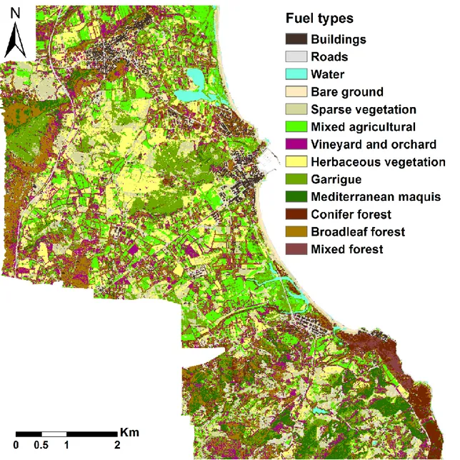
Fig. 1.3. Classification output map for the study area of Siniscola using the Random Forests (RF) algorithm with the subset of variables.
Fig. 1.4. Reclassification in the investigated classes of the Land Use Map (LUM) of Sardinia for the study area of Muravera.
Regarding the LUM of Sardinia (Table 1.8 and Fig. 1.4), the „Mixed agricultural‟ is the fuel type covering the largest extent followed in a much lesser extent by „Garrigue‟. This map showed as the least frequent fuel types „Roads‟ and „Mixed forest‟.
Table 1.8. In the study area of Siniscola, percentage of area covered by each fuel type according to each algorithm and set of variables. ML = Maximum Likelihood; NN = Neural Networks; SVM = Support Vector Machine; RF = Random Forests; LUM = Land Use Map.
Class ML NN SVM RF LUM subset all subset subset all subset
Buildings 6.16 7.77 4.80 4.48 4.68 3.94 7.56 Roads 6.31 8.31 6.95 6.25 11.33 5.95 0.27 Water 0.86 2.72 2.32 1.06 1.31 1.19 1.01 Bare ground 1.52 5.99 1.03 0.71 0.72 0.94 1.64 Sparse vegetation 10.26 7.36 8.41 11.72 9.90 10.58 2.32 Mixed agricultural 8.52 19.98 8.54 9.36 13.67 11.45 41.42 Vineyard and orchard 12.49 4.27 1.83 8.50 7.59 11.49 5.42 Herbaceous vegetation 14.62 10.96 16.10 12.76 10.62 12.92 5.94 Garrigue 17.26 9.72 25.30 21.10 12.54 17.32 17.45 Mediterranean maquis 4.90 9.84 6.82 8.26 11.15 6.71 8.56 Conifer forest 2.79 3.25 5.14 4.78 3.58 3.63 2.74 Broadleaf forest 12.97 7.46 9.88 8.01 9.55 12.05 5.16 Mixed forest 1.34 2.37 2.87 3.01 3.36 1.82 0.51
Also in the study area of Muravera there was a high degree of classification correspondence among maps regarding the fuel types least frequent which were „Bare ground‟, „Water‟ and „Herbaceous vegetation‟ (Tanle 1.9, Fig. 1.5, and Appendix B). Fuel types covering the largest extent were „Mediterranean maquis‟, „Broadleaf forest‟ and „Garrigue‟. The fuel type „Mixed forest‟ is not included in this case because was not found in this study area.
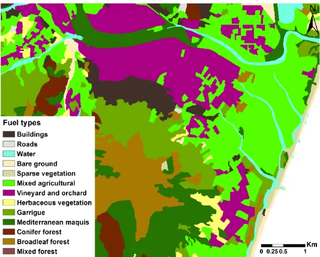
Fig. 1.5. Classification output map for the study area of Muravera using the Random Forests (RF) algorithm with the subset of variables.
Fig. 1.6. Fuel types of the Muravera study area, according to the Land Use Map (LUM) of Sardinia
In this area, the LUM of Sardinia (Table 1.9 and Fig. 1.6) showed „Mixed agricultural‟ as the most frequent fuel type followed by the „Mediterranean maquis‟ whereas „Roads‟ and „Sparse vegetation‟ were present only in a 0.20 and 0.88%, respectively, present in this area.
Table 1.9. In the study area of Muravera, percentage of area covered by each fuel type according to each algorithm and set of variables. ML = Maximum Likelihood; NN = Neural Networks; SVM = Support Vector Machine; RF = Random Forests; LUM = Land Use Map.
Class
ML NN SVM RF
LUM subset all subset subset all subset
Buildings 6.24 5.48 1.97 2.18 3.29 3.34 4.60 Roads 5.91 9.20 5.94 5.29 8.25 6.81 0.20 Water 1.53 2.88 2.48 2.32 2.66 2.35 3.09 Bare ground 1.22 3.42 0.91 0.81 3.59 0.88 1.72 Sparse vegetation 1.91 3.69 3.76 3.23 5.97 5.25 0.88 Mixed agricultural 5.71 4.35 9.19 7.18 3.63 6.48 22.89 Vineyard and orchard 10.25 14.31 18.09 15.36 9.35 9.41 16.53 Herbaceous vegetation 2.67 3.12 3.50 3.22 1.66 2.53 2.01 Garrigue 21.57 4.95 10.27 16.58 10.46 17.42 12.85 Mediterranean maquis 15.54 21.48 16.33 20.16 22.89 15.65 18.96 Conifer forest 5.91 5.95 15.57 10.32 12.39 13.14 2.71 Broadleaf forest 21.53 21.17 12.00 13.33 15.87 16.75 13.57
Regarding the user‟s and producer‟s accuracy, „Water‟ was the class which higher values (Tables 1.10 and 1.11, and Appendices C and D). However, regarding the producer‟s accuracy the most accurately classified fuel types were very different in the two study area: in Siniscola they were „Conifer forest‟, „Garrigue‟ and „Mixed agricultural‟ while in Muravera they were „Herbaceous vegetation‟, „Mixed agricultural‟ and „Sparse vegetation‟. Results regarding the fuel types with higher error of omission were very uneven. In Siniscola the lowest value of producer‟s accuracy was in the fuel
type „Vineyard and orchard‟ with the NN algorithm using the subset of variables (9.09%), but with the RF algorithm using all variables or with the ML algorithm we obtained a 100% of producer‟s accuracy. In Muravera again the NN algorithm with all variables showed the worst performance in this case for the „Conifer forest‟ with a producer‟s accuracy value of 0% while RF with all variables reached a 100% for the same fuel type.
In case of user‟s accuracy, in both areas the fuel types „Mixed Agricultural‟ and „Buildings‟ showed the highest values, whereas „Vineyard and orchard‟ in Siniscola (40%) and „Conifer forest‟ in Muravera (0%) showed the lowest values when they were classified using the NN algorithm with the subset of variables and all variables respectively.
In both, producer‟s and user‟s accuracy, RF showed high values and very balanced for all fuel types, especially when performed with the subset of variables. Conversely, NN showed most uneven results for the different fuel types.
Also in this case we included data from the validation carried out with the Sardinian LUM. The results are very unbalanced showing for some fuel types very high accuracy values, such as „Broadleaf forest‟ and „Water‟ in both areas whereas other fuel types such as „Conifer forest‟ showed very different values in each study area. There were also some fuel types for which producer‟s and user‟s accuracy was very unbalanced, especially in the Siniscola study area („Sparse vegetation‟ and „Roads‟).
Table 1.10. Producer‟s and user‟s accuracy (%) from the classification outputs obtained using the different algorithms in the study area of Siniscola. ML = Maximum Likelihood; NN = Neural Networks; SVM = Support Vector Machine; RF = Random Forests; LUM = Land Use Map.
Class Accuracy ML NN SVM RF LUM subset subset all subset subset all
Buildings Producer's 89.77 85.71 79.12 90.11 89.77 88.64 94.68 User's 91.86 96.30 90.00 94.25 96.34 93.98 69.53 Roads Producer's 81.48 91.96 80.36 91.96 94.44 92.59 15.84 User's 91.67 89.57 86.54 87.29 90.27 90.91 100.00 Water Producer's 100.00 100.00 92.00 100.00 100.00 100.00 81.48 User's 100.00 92.59 82.14 100.00 95.83 100.00 100.00
Bare ground Producer's 83.64 75.00 84.09 70.45 87.27 74.55 60.78
User's 64.79 71.74 56.06 75.61 84.21 83.67 51.67 Sparse vegetation Producer's 54.79 72.60 53.42 73.97 82.19 84.93 1.28 User's 70.18 72.60 68.42 75.00 80.00 70.45 100.00 Mixed agricultural Producer's 91.67 84.85 96.97 90.91 94.44 94.44 97.73 User's 100.00 100.00 65.31 100.00 100.00 100.00 29.86 Vineyard and orchard Producer's 100.00 9.09 81.82 68.18 85.71 100.00 84.00 User's 77.78 40.00 81.82 88.24 100.00 93.33 72.41 Herbaceous vegetation Producer's 94.74 79.31 58.62 75.86 81.58 78.95 12.90 User's 66.67 63.89 73.91 70.97 88.57 93.75 57.14 Garrigue Producer's 97.30 86.84 84.21 100.00 97.30 100.00 65.71 User's 87.80 68.75 80.00 90.48 92.31 94.87 30.26 Mediterranean maquis Producer's 84.78 90.48 88.10 95.24 97.83 95.65 86.11 User's 100.00 79.17 88.10 83.33 95.74 97.78 55.36
Conifer forests Producer's 95.24 90.70 88.37 95.35 100.00 100.00 50.00
User's 93.02 68.42 64.41 85.42 97.67 100.00 38.89
Broadleaf forests
Producer's 84.85 65.71 74.29 65.71 90.91 93.94 94.12 User's 80.00 62.16 89.66 95.83 93.75 100.00 84.21
Mixed forests Producer's 76.32 61.36 65.91 90.91 94.74 100.00 0.00
Table 1.11. Producer‟s and user‟s accuracy (%) from the classification outputs obtained using the different algorithms in the study area of Muravera. ML = Maximum Likelihood; NN = Neural Networks; SVM = Support Vector Machine; RF = Random Forests; LUM = Land Use Map.
Class Accuracy ML NN SVM RF LUM subset subset all subset subset all
Buildings Producer's 85.71 69.23 69.23 76.92 85.71 92.86 100.00 User's 92.31 90.00 52.94 100.00 100.00 100.00 100.00 Roads Producer's 80.00 75.00 54.17 79.17 85.00 65.00 0.00 User's 84.21 72.00 72.22 86.36 85.00 72.22 0.00 Water Producer's 100.00 100.00 100.00 100.00 100.00 100.00 100.00 User's 100.00 96.43 100.00 100.00 100.00 100.00 70.27
Bare ground Producer's 86.67 84.62 76.92 100.00 80.00 80.00 41.67
User's 92.86 78.57 66.67 86.67 85.71 92.31 35.71 Sparse vegetation Producer's 88.89 69.23 84.62 76.92 100.00 100.00 0.00 User's 61.54 90.00 100.00 71.43 81.82 75.00 0.00 Mixed agricultural Producer's 88.24 100.00 90.48 90.48 88.24 82.35 60.00 User's 100.00 84.00 95.00 100.00 93.75 93.33 22.50 Vineyard and orchard Producer's 75.00 85.71 100.00 64.29 87.50 87.50 100.00 User's 80.00 63.16 73.68 75.00 100.00 93.33 66.67 Herbaceous vegetation Producer's 80.00 90.48 90.48 95.24 96.00 92.00 44.00 User's 95.24 90.48 82.61 86.96 92.31 85.19 84.62 Garrigue Producer's 92.31 35.71 64.29 64.29 100.00 76.92 28.57 User's 54.55 50.00 81.82 56.25 81.25 66.67 28.57 Mediterranean maquis Producer's 63.16 69.23 69.23 84.62 100.00 94.74 47.06 User's 80.00 69.23 81.82 73.33 100.00 94.74 72.73
Conifer forests Producer's 68.75 83.33 0.00 83.33 87.50 100.00 100.00
User's 91.67 76.92 0.00 66.67 87.50 84.21 84.21
Broadleaf forests
Producer's 90.91 76.47 94.12 76.47 81.82 81.82 78.26 User's 62.50 92.86 57.14 92.86 81.82 100.00 94.74
4. DISCUSSION
High accuracies were reached by combining multispectral and LiDAR data in the fuel type classification, especially if we compare these results with the LUM of Sardinia which showed very low accuracy coefficients.
The higher values of overall accuracy respect to the Kappa coefficient are common since latter is a more conservative measure than the overall classification accuracy. According to both accuracy coefficients (overall accuracy and Kappa coefficient), the best method for classifying this kind of data in these fuel types is the RF algorithm, followed by the SVM algorithm. The least performing algorithm was the NN contrary to what Frizzelle and Moody (2001) found in their study of characterization of land cover from multispectral data. In their work they obtained better results with the NN algorithm than the ML maybe because they used few variables and the classified only eight land cover categories. However, in agreement with our results, García et al. (2011) found in their study combining also LiDAR and Multispectral data, that SVM had higher potential for combing different data sources than ML. Also in accordance with our results, in the study of Pal and Mather (2005) RF showed accuracy coefficients slightly better than SVM, even if also in this case the classification was carried out using only multispectral data for seven classes.
The most similar work to our study is the one carried out by Reese et al. (2014) since they used Spot-5 and LiDAR data to classify 12 classes of vegetation using the RF algorithm. However, they made it for alpine vegetation which includes mainly different types of herbaceous vegetation and shrubs and two classes of broadleaf forests. Their accuracies coefficients were much lower than ours (63.1% of overall accuracy).
Also the classifications and the LUM of Sardinia differ in the fuel distribution of the study areas (Figs. 1.3, 1.4, 1.5, and 1.6), probably due to the coarser resolution of the latter.
Regarding the performance per fuel type, besides „Water‟, which showed very high accuracies in both areas, the rest of fuel types showed very different values in each study area. This is probably because of the very different spatial distribution of fuel types in each area, which makes easier to define certain fuel types in each area.
However we selected these two study areas for this reason (different distribution of fuels characteristics of the island) and even if the results differ, in both cases showed high values of accuracy. Also in our study RF is the algorithm showing the most balanced performance regarding the results per fuel types with high values of both, producer‟s and user‟s accuracy.
5. CONCLUSIONS
Regarding the objective of this study, we can conclude that it is possible to create high accuracy fuel maps by combining multispectral and LiDAR data and the resulting maps improve the available information until now.
Even if in this case we applied the methodology only to a small study area, the same methodology could be extended to other areas. Moreover, if new LiDAR data will be available for the whole island in the next years, we could update the fuel maps by following this methodology.
In this study, the RF algorithm carried out with a subset of variables showed the best performance for the fuel type classification. However, RF with all variables performs a reasonably accurate classification (even if the results are not good as with selected variables). Therefore, since the selection of variables suppose extra-work and time, for a quick classification or if the classification should be done for lots of different areas, this methodology could be applied.
Further work should be focus on the improvement of the variable selection for automatize the process and optimize the results.
Acknowledgments
We would like to acknowledge the Autonomous Region of Sardinia for providing the LiDAR data and the orthofotos. In addition, we also thank the Forest Service of Sardinia for the Spot imagery.
References
Ager AA, Preisler HK, Arca B, Spano D, Salis M (2014) Wildfire risk estimation in the Mediterranean area. Environmetrics 25, 384–396. doi:10.1002/env.2269.
Alcasena FJ, Salis M, Ager AA, Arca B, Molina D, Spano D (2015) Assessing
Landscape Scale Wildfire Exposure for Highly Valued Resources in a Mediterranean Area. Environmental Management 55, 1200–1216.
doi:10.1007/s00267-015-0448-6.
Arca B, Bacciu V, Pellizzaro G, Salis M, Ventura A, Duce P, Brundu G (2009) Fuel model mapping by Ikonos imagery to support spatially explicit fire simulators. In: Spano et al. (eds) „International Conference on Fire Behaviour and Risk‟, Matera. pp 92–98.
Arca B, Duce P, Pellizzaro G, Bacciu V, Salis M, Spano D (2007) Evaluation of Farsite Simulator in Mediterranean maquis. International Journal of Wildland Fire 16, 563–572. doi:10.1071/WF06070.
Arroyo LA, Pascual C, Manzanera A (2008) Fire models and methods to map fuel types: The role of remote sensing. Forest Ecology and Management 256, 1239– 1252. doi:10.1016/j.foreco.2008.06.048.
Autonomous Region of Sardinia (2008) Carta dell‟Uso del Suolo in scala 1:25.000. http://www.sardegnageoportale.it/index.php?xsl=1598&s=291548&v=2&c=8831 &t=1.
Bajocco S, Dragoz E, Gitas I, Smiraglia D, Salvati L, Ricotta C (2015) Mapping forest fuels through vegetation phenology: The role of coarse-resolution satellite time-series. PLoS ONE 10, 1–14. doi:10.1371/journal.pone.0119811.
Breiman L (2001) Random forests. Machine Learning 45, 5–32. doi:10.1023/A:1010933404324.
Chuvieco E (2010) „Teledetección ambiental. La observación de la Tierra desde el Espacio.‟ (Ariel Ciencia: Barcelona)
Chuvieco E, Wagtendok J, Riaño D, Yebra M, Ustin SL (2009) Estimation of fuel conditions for fire danger assessment. In: Chuvieco (ed) „Earth observation of wildland fires in Mediterranean ecosystems‟ pp. 83–96. (Springer: Berlin Heidelberg)
Congalton RG (1991) A review of assessing the accuracy of classifications of remotely sensed data. Remote Sensing of Environment 37, 35–46. doi:10.1016/0034-4257(91)90048-B.
EEA (2011) Version 15 of raster data on land cover for the corine land cover 2006 inventory. European Environmental Agency, http://www.eea.europa.eu/data-and-maps/data/corine-land-cover-2006-raster-1.
Falkowski MJ, Evans JS, Martinuzzi S, Gessler PE, Hudak AT (2009) Characterizing forest succession with lidar data: An evaluation for the Inland Northwest, USA.
Remote Sensing of Environment 113, 946–956. doi:10.1016/j.rse.2009.01.003.
Foody GM (2006) What is the difference between two maps? A remote senser‟s view.
Journal of Geographical Systems 8, 119–130. doi:10.1007/s10109-006-0023-z.
Frizzelle BG, Moody A (2001) Mapping Continuous Distributions of Land Cover : A Comparison of Maximum-Likelihood. Estimation and Artificial Neural Networks.
Photogrammetric Engineering & Remote Sensing 67, 693–705.
García M, Riaño D, Chuvieco E, Salas J, Danson FM (2011) Multispectral and LiDAR data fusion for fuel type mapping using Support Vector Machine and decision rules. Remote Sensing of Environment 115, 1369–1379.
doi:10.1016/j.rse.2011.01.017.
Isenburg M (2015) LAStools - Efficient Tools for Lidar Processing. Version 140329. http://lastools.org.
Koetz B, Morsdorf F, Van Der Linden S, Curt T, Allgöwer B (2008) Multi-source land cover classification for forest fire management based on imaging spectrometry and LiDAR data. Forest Ecology and Management 256, 263–271.
Lasaponara R, Lanorte A (2007a) Remotely sensed characterization of forest fuel types by using satellite ASTER data. International Journal of Applied Earth Observation
and Geoinformation 9, 225–234. doi:10.1016/j.jag.2006.08.001.
Lasaponara R, Lanorte A (2007b) On the capability of satellite VHR QuickBird data for fuel type characterization in fragmented landscape. Ecological Modelling 204, 79– 84. doi:10.1016/j.ecolmodel.2006.12.022.
Mallinis G, Galidaki G, Gitas I (2014) A Comparative Analysis of EO-1 Hyperion, Quickbird and Landsat TM Imagery for Fuel Type Mapping of a Typical Mediterranean Landscape. Remote Sensing 6, 1684–1704. doi:10.3390/rs6021684.
Mallinis G, Mitsopoulos ΙD, Dimitrakopoulos AP, Gitas IZ, Karteris M (2008) Local-Scale Fuel-Type Mapping and Fire Behavior Prediction by Employing High-Resolution Satellite Imagery. IEEE Journal of Selected
Topics in Applied Earth Observations and Remote Sensing 1, 230–239.
doi:10.1109/JSTARS.2008.2011298.
Marino E, Ranz P, Luis J, Ángel M, Esteban J, Madrigal J (2016) Remote Sensing of Environment Generation of high-resolution fuel model maps from discrete airborne laser scanner and Landsat-8 OLI : A low-cost and highly updated methodology for large areas. Remote Sensing of Environment 187, 267–280. doi:10.1016/j.rse.2016.10.020.
Martin M., Newman S., Aber J., Congalton R. (1998) Determining forest species composition using high spectral resolution remote sensing data. Remote Sensing of
Environment 65, 249–254. doi:10.1016/S0034-4257(98)00035-2.
McGaughey RJ (2014) FUSION/LDV: Software for LIDAR Data Analysis and Visualization. 154.
Mountrakis G, Im J, Ogole C (2011) Support vector machines in remote sensing: A review. ISPRS Journal of Photogrammetry and Remote Sensing 66, 247–259. doi:10.1016/j.isprsjprs.2010.11.001.
Ottmar RD, Alvarado E (2004) Linking Vegetation Patterns to Potential Smoke Production and Fire Hazard 1. USDA Forest Service, Pacific Northwest Research Station, General Technical Report PSW-GTR-193. (Seattle, WA)
Otukei JR, Blaschke T (2010) Land cover change assessment using decision trees, support vector machines and maximum likelihood classification algorithms.
International Journal of Applied Earth Observation and Geoinformation 12, 27–
31. doi:10.1016/j.jag.2009.11.002.
Pal M (2005) Random forest classifier for remote sensing classification. International
Journal of Remote Sensing 26, 217–222. doi:10.1080/01431160412331269698.
Pal M, Mather PM (2005) Support vector machines for classification in remote sensing. International Journal of Remote Sensing 26, 1007–1011. doi:10.1080/01431160512331314083.
Qiu F, Jensen JR (2004) Opening the black box of neural networks for remote sensing image classification. International Journal of Remote Sensing 25, 1749–1768. doi:10.1080/01431160310001618798.
R Core Team (2016) R: A language and environment for statistical computing. http://www.r-project.org/.
Reese H, Nyström M, Nordkvist K, Olsson H (2014) Combining airborne laser scanning data and optical satellite data for classification of alpine vegetation. International
Journal of Applied Earth Observation and Geoinformation 27, 81–90.
doi:10.1016/j.jag.2013.05.003.
Richter R, Schläpfer D (2012) ATCOR-2/3 User Guide, Version 8.2.0. 223.
Salis M, Ager AA, Arca B, Finney MA, Bacciu V (2013) Analyzing wildfire exposure to human and ecological values in Sardinia, Italy. International Journal of