Bravo, F., & Crudu, F. (2012). Efficient Bootstrap with Weakly Dependent Processes. COMPUTATIONAL STATISTICS & DATA ANALYSIS, 56, 3444-3458.
This is the peer reviewd version of the followng article:
Efficient Bootstrap with Weakly Dependent Processes
Published:
DOI:10.1016/j.csda.2010.07.021
Terms of use:
Open Access
(Article begins on next page)
The terms and conditions for the reuse of this version of the manuscript are specified in the publishing policy. Works made available under a Creative Commons license can be used according to the terms and conditions of said license. For all terms of use and more information see the publisher's website.
Availability:
This version is available http://hdl.handle.net/11365/1005853 since 2017-04-29T10:28:51Z
Discussion Papers in Economics
Department of Economics and Related Studies University of York
Heslington York, YO10 5DD
No. 12/08
Efficient bootstrap with weakly dependent
processes
By
E¢ cient bootstrap with weakly dependent
processes
Francesco Bravo
University of York
Federico Crudu
yUniversity of Groningen
AbstractThe e¢ cient bootstrap methodology is developed for overidenti…ed moment conditions models with weakly dependent observation. The resulting bootstrap procedure is shown to be asymptotically valid and can be used to approxi-mate the distributions of t-statistics, J statistic for overidentifying restrictions, and Wald, Lagrange multiplier and distance statistics for nonlinear hypotheses. The asymptotic validity of the e¢ cient bootstrap based on a computationally less demanding approximate k-step estimator is also shown. The …nite sam-ple performance of the proposed bootstrap is assessed using simulations in an intertemporal consumption based asset pricing model.
Key words and Phrases: -mixing, Consumption CAPM, GEL, GMM, Hy-pothesis testing
Corresponding author. Department of Economics and Related Studies, University of York, York YO10 5DD, United Kingdom. email [email protected]
yDepartment of Economics and Econometrics, University of Groningen, 9747 AE Groningen, The Netherlands. email: [email protected]
1
Introduction
This paper develops Brown and Newey’s (2002) e¢ cient bootstrap methodology to possibly overidenti…ed moment conditions models with weakly dependent observa-tions. The e¢ cient bootstrap di¤ers from the traditional one in that it uses as resampling probabilities those obtained by estimating the unknown distribution of the observations subject to the constraint implied by the moment conditions them-selves. The resulting estimator is typically more e¢ cient than the empirical dis-tribution function used in the traditional bootstrap as the nonparametric estima-tor of the distribution of the observation, hence the term e¢ cient, although some-times in the statistical literature the same bootstrap methodology is called “biased” (Hall and Presnell, 1999). In this paper the estimator we consider is the gener-alised empirical likelihood estimator of Newey and Smith (2004). This estimator is very general and includes a number of well-known estimators including empirical likelihood (Owen, 1988), exponential tilting (Efron, 1981), and euclidean likelihood (Owen, 1991).
In this paper we make two main contributions: …rst we generalise the e¢ cient bootstrap to weakly dependent observations. To be speci…c we prove the asymptotic validity of the e¢ cient bootstrap approximation to the true distribution of the gener-alised method of moment (GMM) estimator. We also consider testing and prove the asymptotic validity of the bootstrap approximation for t-statistics, Hansen’s (1982) J statistic for overidentifying restrictions, and for Wald, Lagrange multiplier and dis-tance statistics for nonlinear hypotheses. This extension is theoretically interesting and empirically relevant in economics and …nance where most of the observed time series exhibit some form of temporal dependence and most of the hypotheses of in-terest are typically composite. Second we provide Monte Carlo evidence about the …nite sample performance of the proposed bootstrap and compare it with that of the standard bootstrap. The results of the simulations are encouraging and suggest that the proposed bootstrap has competitive …nite sample properties compared to those
of the standard bootstrap.
The results of this paper complement those obtained by Flachaire (2005) and Godfrey and Tremayne (2005) among others. These authors recommend using wild (block) bootstrap in the context of (dynamic) heteroskedastic linear regression mod-els. The wild bootstrap however cannot accommodate potential endogeneity of re-gressors, and, more generally, it requires a regression type of model. In contrast the method proposed in this paper applies to more general statistical models and can accommodate endogeneity; for example nonlinear instrumental variable estimation is allowed.
It is important to note that the results of this paper are related to those obtained by Allen, Gregory and Shimotsu (2005). They propose to use the same type of e¢ cient bootstrap used in this paper. There are however a number of important di¤erences between their paper and ours. First, our e¢ cient bootstrap uses the estimated probabilities to resample the moment indicators, whereas Allen et al. (2005) use the estimated probabilities only to centre the resampled moment indicator. Thus our bootstrap method is the direct extension of that proposed by Brown and Newey (2002). Second we consider e¢ cient bootstrap GMM inferences for possibly nonlinear statistical hypotheses. Third we consider k-step versions of the e¢ cient bootstrap GMM estimators. Finally we resample using the overlapping blocks scheme (the so-called moving block bootstrap) as opposed to nonoverlapping blocks scheme used by Allen et al. (2005). On the other hand we consider stationary -mixing observations, instead of the more general possibly nonstationary near epoch dependent speci…cation used by Allen et al. (2005).
The rest of the paper is structured as follows: Section 2 brie‡y introduces the statistical model and GMM estimation and inference. Section 3 describes the e¢ cient bootstrap and develops the necessary asymptotic theory. Section 4 reports the results of the simulations and some concluding remarks. An appendix contains all the proofs and some details about the arti…cial data used in the simulations.
2
GMM estimation and inference
Let fztgt2Z denote a sequence of Rdz-valued random vectors de…ned on some
proba-bility space ( ; F; P ). Let 2 B Rk denote a parameter vector, and let g (zt; ) :
Rd B
! Rl (l k)
denote a vector of (FnBorel-measurable for each 2 B) func-tions satisfying the possibly overidenti…ed moment condifunc-tions
E [g (zt; 0)] = 0; (1)
where the expectation is with respect to the unknown distribution F of zt and 0 is
the unique unknown parameter.
Given an observed sample fztgTt=1, the two-step (e¢ cient) GMM estimators b for 0 is de…ned as
b = arg min
2B bg( )
0b e 1bg b ;
where bg( ) = PTt=1gt( ) =T, gt( ) = g (zt; ), b e is a consistent estimator of
the covariance matrix ( 0) := limT !1V T1=2bg( 0) and e any preliminary T1=2 -consistent estimator. Under mild regularity conditions Hansen (1982) shows that
T1=2 b 0 ! N 0; (d 0) 1 ;
where ( 0) := G ( 0)0 ( 0) 1G ( 0) and G ( 0) := E [@bg( 0) =@ 0]. Associated with the two-step GMM estimator b there is the so-called J -statistic for overidentify-ing restriction J b , where J ( ) = Tbg( )0b ( ) 1bg( ), which can be used to test the correct speci…cation of (1) since Hansen (1982) shows that
J b !d 2l k:
Let h ( ) : B ! Rp (p k) denote a vector of continuously di¤erentiable on B
functions, and suppose that we want to test the hypothesis H0 : h ( 0) = 0. As in
multiplier and likelihood ratio statistics: W b = T h b 0 H b b b 1 H b 0 1 h b ; (2) LM e = Tbg e 0 b e 1 b G e b b 1 b G e 0b e 1 bg e and D e; b = JT e JT b ;
where H ( ) = @h ( ) =@ 0, e is the constrained GMM estimator for 0 de…ned as
e = arg min
2Bbg( )
0b e 1bg( ) subject to h ( ) = 0; (3)
b
G ( ) = PTt=1@gt( ) =@ 0T. Under mild regularity conditions Newey and West
(1987a) show that
W b ; LM e ; D e; b !d 2p:
GMM is widely used in empirical economics and …nance -see the special issue of the Journal of Business and Economic Statistics 2002 and especially the monograph of Hall (2005) for a survey of recent applications and development of GMM. There exists however Monte Carlo evidence, see for example the special issue of the Journal of Business and Economic Statistics 1996, showing that asymptotic theory might not provide a good approximation to the …nite sample behaviour of GMM estimators and associated statistics.
In order to improve the …nite sample behaviour of GMM statistics one possibility is to use bootstrap methods. Indeed Hall and Horowitz (1996), Andrews (2002) and more recently Inoue and Shintani (2006) use the block bootstrap to obtain asymp-totic re…nements to the distributions of Hansen’s (1982) J statistic for overidentifying restrictions and symmetrical t statistics. All these authors base the bootstrap estima-tion on centred sample moment condiestima-tions. Centring is not necessary to obtain the asymptotic validity of the bootstrap GMM t-statistic (Hahn, 1996), but it is neces-sary to obtain asymptotic re…nements (Hall and Horowitz, 1996). It is also necesneces-sary to obtain asymptotic validity of the bootstrap J statistic (Brown and Newey, 2002).
An alternative approach to centring is to use a di¤erent estimator of the unknown distribution of the observations that automatically centres the resampled moment indicators, as originally suggested by Brown and Newey (2002) in the context of for identically and independently observations.
3
E¢ cient block bootstrap
In this section we introduce a modi…cation of Brown and Newey’s (2002) e¢ cient bootstrap that is based on the generalised empirical likelihood (GEL) estimator of Newey and Smith (2004) and can be used with weakly dependent observations. Let (v)denote a function of a scalar v that is concave on its domain, an open interval V containing 0, and let j(v) = dj (v) =dvj. Examples of (v) are log (1 v)(empirical
likelihood), exp (v)(exponential tilting) and (1 + v)2=2(euclidean likelihood). To capture the weakly dependent structure of the observations we consider over-lapping blocks of observations; let m = m (T ) and bi = z0i; :::; zi+m 10
0
be the i-th block of m consecutive observations for 1 i Q = T m + 1. De…ne now the blockwise moment function
(bi; ) := i( ) = m
X
j=1
g (zi+j 1; ) =m; (4)
and note that if (1) holds then E [ i( 0)] = 0. The (blockwise) GEL estimator of
the unknown distribution F consistent with (1) is b Fb(z) = Q X i=1 m X j=1 biIfzi+j 1 zg =m; where bi = 1 b0 i b = Q X i=1 1 b0 i b (5)
are the so-called GEL implied probabilities, b = arg max 2 bV
Q
PQ
i=1 0 i b =Q,
b
the e¢ cient GMM or any asymptotically equivalent GEL estimators de…ned as b = arg min 2BPQi=1 b0
i( ) =Q. Note that the computation of b is straightforward
because of the global concavity of ( ), and that
b = ( 0) 1 b + ob p(1) ; (6)
where b ( ) =PQi=1 i( ) =Q (Bravo, 2009).
The e¢ cient block bootstrap (EBB henceforth) uses the GEL implied probabilities bi to resample the blocks bi to obtain n blocks bi with n = bT=mc where b c is the
integer part function, that is each bootstrap block bi is drawn independently with replacement with probability Pr bj = bi = bi i = 1; :::; Q, j = 1; :::; n. Given bi
(i = 1; :::; n) we can construct EBB analogues of the blockwise moment indicators (4), that is i ( ) (i = 1; :::; n). These moment indicators satisfy the sample moment
condition because E [ i ( )] = 0 when = b by construction (by (6) and Lemma 4 in the Appendix), where E denote the expectation relative to the EBB bootstrap distribution conditional on the original sample.
The EBB two-step GMM estimator b is de…ned as b = arg min 2B b ( )0 b e 1 b ( ) ; (7)
where e is a preliminary consistent EBB GMM estimator, such as an EBB one-step GMM estimator. The latter can be de…ned in an analogous way as
b = arg min
2B
b
( )0cW b ( ) ;
where cW is a possibly random positive semide…nite matrix. Furthermore we can de…ne the EBB t-statistic and J statistic for overidentifying restrictions as
t = T1=2 bj bj = b b 1 jj 1=2 j = 1; :::; k; (8) J b = T b b 0b b 1 b b ;
where, with a slight abuse of notation, mn = T . Thus an EBB t-test and J test reject, respectively, if jtj qbt and J qbJ, where qbt and qbJ are the 1 percentile
of the distributions of t and J b obtained by computing (8) B times.
To de…ne EBB analogues of the three GMM based statistics (2) that can be used to test H0 : h ( 0) = 0 let ei = 1 e0 i e = Q X i=1 1 e0 i e (9)
denote the restricted implied probabilities, where e = arg max 2 bV
Q
PQ
i=1 0 i e =Q
a and e is any two-step constrained estimator for 0, such as the constrained GMM
estimator de…ned in (3)or any asymptotically equivalent blockwise GEL estimators de…ned as e = arg min 2BPQi=1 e0
i( ) =Q subject to h ( ) = 0. As with the
unconstrained EBB two-step GMM estimator we use ei to obtain moment functions
i ( ) (i = 1; :::; n) that by construction E [ i ( )] = 0 when = e.
The EBB constrained two step GMM estimator is e = arg min
2B
b
( )0b 1b b ;
where is a preliminary consistent EBB constrained GMM estimator. The EBB analogues of (2) are W b = T hh b h b i0 H b b b 1 H b 0 1h h b h b i; LM e = T b e 0b e 1Gb e b e 1Gb e 0 b e 1 b e and (10) D e; b = J e J b :
Thus an EBB Wald, Lagrange multiplier and distance tests, say S, reject if S bqs where qbs is the 1 percentile of the distribution obtained by computing B times
Like any other resampling method EBB can be computationally very demanding when applied to nonlinear moment conditions models. One way to reduce the com-putational cost is to follow Davidson and MacKinnon’s (1999) suggestion and use an approximate k-step (k = 1; 2; :::) EBB two-step GMM estimator alternative to (the fully optimised) , that is
(j) = (j 1) b (j 1) 1Gb (j 1) 0b (j 1) 1b (j 1) 1 j k
where (0) = and can be either the unconstrained or constrained two-step GMM estimator.
Asymptotic theory
The following assumptions are standard in the GMM/GEL literature on nonlinear (di¤erentiable) moment condition models with stationary weakly dependent obser-vations - see for example Wooldridge (1994), Hall (2005), and Politis and Romano (1992), and Goncalves and White (2004) for a bootstrap analogue.
A1 fztgt2Z is a strictly stationary strong mixing sequence of size = ( 2)where
> 2;
A2 (i) The parameter space B is compact, (ii) 0 2 B is the unique solution to E [gt( 0)] = 0, (iii) gt( ) is continuous a:s: at each 2 B , (iv) (a)
E sup 2Bkgt( )k < 1, (b) E
h
kgt( 0)k 2 + i
< 1 for some > 0 (v) ( 0) := limT !1V n1=2bg( 0) is positive de…nite,
A3 (i) 0 2 int (B) , (ii) gt( )is continuously di¤erentiable a:s: in a convex
neigh-bourhood N of 0 8t and 8 2 N (iii) E sup 2N k@gt( ) =@ 0k 2
< 1 (iv) rank [G ( 0)] = k where G ( 0) = E [@gt( 0) =@ 0],
A4 ( ) is twice continuously di¤erentiable in an open neighbourhood of 0, and
The following theorem establishes the asymptotic validity of the EBB two-step GMM estimator b and of the J statistic for overidentifying restrictions J b . Theorem 1 Suppose that A1-A4 hold. If m = o T1=2 then
sup x2Rk P hT1=2 b b xi PhT1=2 b 0 x i p ! 0; sup x2R+ P hJ b xi P hJ b xi ! 0:p
The following theorem establishes the asymptotic validity of the EBB Wald, La-grange multiplier and distance statistics W b , LM e and D e; b :
Theorem 2 Suppose that A1-A4 hold. If rank [H ( 0)] = p and m = o T1=2 then
sup x2R+ P hW b xi P hW b xi ! 0;p sup x2R+ P hLM e xi P hLM e xi ! 0p and sup x2R+ P hD e ; b xi P hD e; b xi ! 0:p
Finally the following theorem shows that the k-step (k = 1; 2; ::) EBB two-step GMM estimator (k) achieves the same asymptotic accuracy as that of the fully
optimised one .
Theorem 3 Suppose that A1-A4 hold. If m = o T1=2 then
sup
x2Rk
P T1=2 (k) x P T1=2 x ! 0:p
4
Monte Carlo evidence
In this section we use simulations to evaluate the …nite sample properties of the EBB and compare them with those obtained by the standard block bootstrap (BB henceforth) and by standard asymptotic approximations. We focus on the t and J
statistics partly because they are routinely used in empirical work and partly because of their well documented …nite sample over-rejections problems.
We consider an intertemporal consumption based asset pricing model used by Tauchen (1986), Kocherlakota (1990) and Wright (2003) among others. Consumption and dividend growth are assumed to follow a …rst order vector autoregression
2 4 log (ct=ct 1) log (dt=dt 1) 3 5 = 2 4 c0 d0 3 5 + 0 2 4 log (ct 1=ct 2) log (dt 1=dt 2) 3 5 + 2 4 "ct "dt 3 5 ; (11) where ctis consumption, dtis dividend, 0is a 2 2 matrix of constants and ["ct; "dt]0
N (0; 0). Returns are generated so as to satisfy the stochastic Euler equation
Eh 10(ct=ct 1) 20rt 1sjIt 1
i
= 0 (12)
where 0 = [ 10; 20]0 is the unknown parameters vector, rt is an s-dimensional vector
of returns, 1sis an s-dimensional vector of ones and It 1is the information set at time
t 1. To generate consumption and returns time series consistent with both (11) and (12) we use the same method proposed by Tauchen (1986) and Tauchen and Hussey (1991). This method …ts a 16 state Markov chain to [log (ct=ct 1) ; log (dt=dt 1)]0 to
approximate (11) and then uses numerical methods to approximate the expectation in (12) : The resulting (discretised) system of equations is then used to obtain the prices pt (and hence the returns rt) of stocks and risk-free bonds in each time period
(see the Appendix for some details).
We consider two returns: one based on a stock, say rs
t, and one risk free, say r f t. Estimation of 0 is based on bg( 0) = T X t=1 ft( 0) rt zt 1=T; (13) where ft( 0) = 10(ct=ct 1) 20, rt = h rs t; r f t i0
, is the Kronecker product, and zt = [1; rt0; ct=ct 1]0 is a vector of so-called instruments. Thus (13) consists of 8
is 6. To compute the covariance ( 0)in the two-step GMM we use the Newey-West estimator (Newey and West, 1987b) , whereas we use a blockwise bootstrap covari-ance estimator either centred as in Politis and Romano (1992) or with the implied probabilities bi in the bootstrap two-step GMM. These estimators are asymptoti-cally equivalent for m = o T1=2 and have the same optimal block length parameter
m = T1=3 for any choice of …nite > 0. We consider two b
i, namely bELi = Q 1 1 b0 i b 1 ; bEUi = 1 bb 0 b b 1 i b =hQ 1 J b i;
which correspond to empirical likelihood (EL) and euclidean likelihood (EU), respec-tively. Note that the latter does not require to numerically …nd b because in this case b = b b 1 bb exactly.
In the simulations we consider two parameterisations of (11) and (12) namely Case 1. 0 = [0:97; 1:36]0, 0 = [0:018; 0:013]0, 0 = 2 4 0:5 0:00 0:00 0:5 3 5 , 0 = 2 4 0:01 0:005 0:005 0:01 3 5 ; and Case 2. 0 = [0:97; 0:36]0, 0 = [0:02; 0:03]0, 0 = 2 4 0:1 0:05 0:20 0:12 3 5 , 0 = 2 4 0:01 0:02 0:02 0:05 3 5 ;
which are in the same spirit of those used by Tauchen (1986) and Kocherlakota (1990), respectively. The sample sizes are T = 100 and T = 400, and the block length parameter m is chosen using Newey and West’s (1994) method. The number of bootstrap repetitions is 500 and the number of Monte Carlo replications is 5000.
The results of the simulations are presented using the graphical methods proposed by Davidson and MacKinnon (1998). To save space we report only the results for Case 2 and T = 100. The results for Case 1 and T = 400 are very similar and
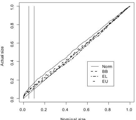
0.0 0.2 0.4 0.6 0.8 1.0 0 .0 0 .2 0 .4 0 .6 0 .8 1 .0 Nominal size A ct u a l size Norm BB EL EU
Figure 1: P-value plots of the t-statistics for H0 : 1 = 10. The two vertical lines
correspond to the 0.05 and 0.10 nominal size.
available upon request. Figures 1-3 show the p-value plots of the two t and J sta-tistics. These plots show the empirical distribution function bF (xi)of the p-values of
the simulated statistics against the set of points xi (i = 1; :::; l) in the (0; 1) interval
with l = 1000. The closer is the plot to the 45-degree line the more accurate is the corresponding approximation. In the plots the solid lines correspond to the asymp-totic approximation (“Norm” or “ 2
6” in the legend), the dashed lines to the block
bootstrap approximation (“BB” in the legend), the two-dash lines to the empirical likelihood based e¢ cient bootstrap approximation (“EL”in the legend) and the dot-dash lines to the euclidean likelihood e¢ cient bootstrap approximation (“EU”in the legend).
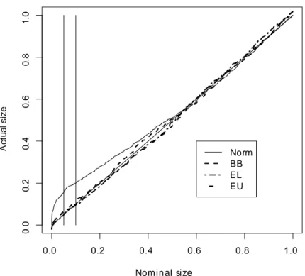
0.0 0.2 0.4 0.6 0.8 1.0 0 .0 0 .2 0 .4 0 .6 0 .8 1 .0 Nominal size A ct u a l size Norm BB EL EU
Figure 2: P-value plots of the t-statistics for H0 : 2 = 20. The two vertical lines
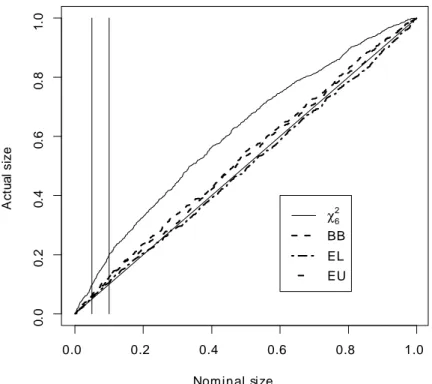
0.0 0.2 0.4 0.6 0.8 1.0 0 .0 0 .2 0 .4 0 .6 0 .8 1 .0 Nominal size A ct u a l size χ6 2 BB EL EU
Figure 3: P-value plots of the J -statistics. The two vertical lines correspond to the 0.05 and 0.10 nominal size.
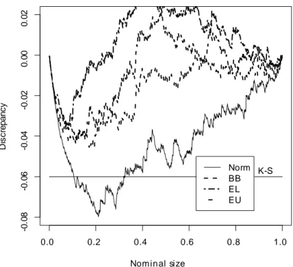
Figures 1-3 show that the t and J statistics based on the asymptotic approximation over-reject, whereas those based on the three block bootstrap approximations perform signi…cantly better, particularly those based on EL. For example the actual size of the J-statistic at the 0.05 nominal level is 0.113 whereas the size of the three bootstrapped J-statistics are 0.052 for that based on EL, 0.059 for that based on EU and 0.061 for that based on BB. Figures 4-6 report the p-value discrepancy plots, which show the discrepancy of bF (xi) xi against xi. The …gures also feature the 0.05 critical value
of the Kolmogorov-Smirnov (KS)-type statistic max
i F (xb i) xi ; (14)
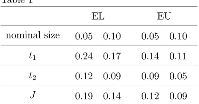
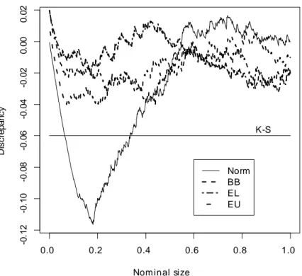
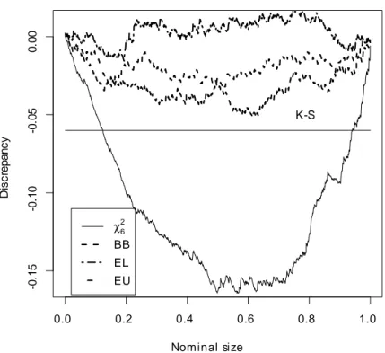
which is used to assess whether the discrepancies can be explained by experimental randomness. Figures 4-6 show that the discrepancies for the three bootstrap proce-dures are not signi…cant. Indeed the p-values of (14) are typically above 0.50. The only exception is for the J statistic based on BB whose p-value is around 0.13, which indicates that in this case the BB approximation is less satisfactory. Figures 4-6 also con…rm that among the three di¤erent block bootstraps the two based on EBB have smaller p-value discrepancies (with those based on EL having the smallest dis-crepancies), implying an overall better …nite sample approximation to the unknown distributions of both the t and J statistics. As a further indication of the better quality of approximations obtained using EBB we have computed the probabilities of BB leading to size distortions that could have been avoided using both EL-EBB and EU-EBB. Table 1 reports these probabilities for the conventional 0.05 and 0.10 nominal sizes and both the t and J statistics.
Table 1 EL EU nominal size 0.05 0.10 0.05 0.10 t1 0.24 0.17 0.14 0.11 t2 0.12 0.09 0.09 0.05 J 0.19 0.14 0.12 0.09
tjis the BB t-statistic for H0: j= j0(j 1;2)and J is the BB J -statistic.
Table 1 shows that if we use for example EL-EBB instead of BB for testing H0 : 1 = 10 we are 24% less likely to have a size distortion at the 0.05 nominal size. Likewise
if we use EU-EBB for the J -statistic we are 9% less likely to have a size distortion at the 0.10 nominal size.
Before we consider the …nite sample power of the t and J statistics, it should be noted that although the various block bootstrap procedures improve considerably their …nite sample behaviour, some small size distortions are still present, particularly for the J statistic with BB. However this fact seems to be typical of overidenti…ed moment conditions models and is consistent for example with the …ndings of Hall and Horowitz (1996).
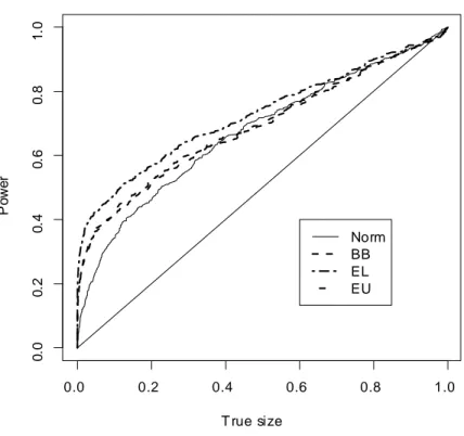
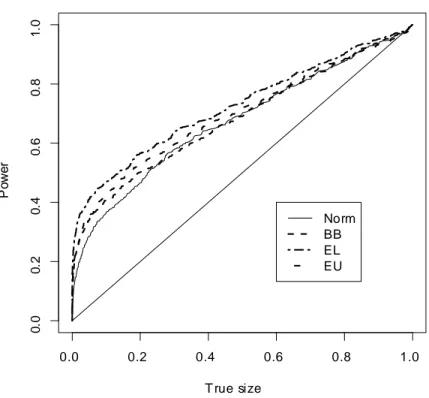
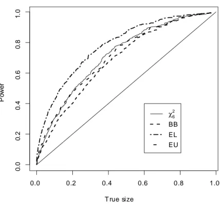
Figures 7-9 show the size-power curves, which plot the power of a test statistic against its true size. The …gures show that in terms of power EL based EBB (EL-EBB henceforth) uniformly dominates the other procedures for a given true size; for example in Figure 7 the t-statistic based on EL-EBB is on average about 18% more powerful than the one based on the normal approximation, whereas in Figure 10 the J statistic based on EL-EBB is on average around 32% more powerful than the one based on BB. These plots also show that neither of the other two block bootstrap approximations dominate the one based on the asymptotic distribution. However the statistics based on EU-EBB are more powerful than those based on BB approximation (from around 5% (on average) in Figure 7 to around 12% (on average) in Figure 9).
0.0 0.2 0.4 0.6 0.8 1.0 -0 .08 -0 .06 -0 .04 -0 .02 0. 00 0. 02 Nominal size D iscr e p a n cy K-S Norm BB EL EU
Figure 4: P-value discrepancy plots of the t statistic for H0 : 1 = 10. The horizontal
0.0 0.2 0.4 0.6 0.8 1.0 -0 .12 -0 .10 -0 .08 -0 .06 -0 .04 -0 .02 0. 00 0. 02 Nominal size D iscr e p a n cy K-S Norm BB EL EU
Figure 5: P-value discrepancy plots of the t statistic for H0 : 2 = 20. The horizontal
0.0 0.2 0.4 0.6 0.8 1.0 -0 .15 -0 .10 -0 .05 0. 00 Nominal size D iscr e p a n cy K-S χ6 2 BB EL EU
Figure 6: P-value discrepancy plots of the J statistic. The horizontal line corresponds to the 0.05 critical value of the K-S statistic (14).
0.0 0.2 0.4 0.6 0.8 1.0 0 .0 0 .2 0 .4 0 .6 0 .8 1 .0 T rue size P o w er Norm BB EL EU
Figure 7: Size-power curves of the t statistic for H0 : 1 = 10.
This suggests that, in general, the e¢ cient bootstrap method of this paper has a clear advantage over the standard bootstrap in terms of power.
We now consider the one-step version of both BB and EBB based GMM. These estimators are computationally very attractive because they are simply the …rst (boot-strap) iteration from the original GMM estimator. Overall the …nite sample prop-erties of the resulting bootstrapped t-statistics are very similar. Therefore we only report the results for the t-statistic for H0 : 2 = 20 and the J -statistic. Figures
10-11 show the di¤erences between the p-value discrepancy plots of the fully opti-mised with those based on the one-step version of the bootstrap, with a negative value indicating a larger discrepancy for the one-step estimator. It is clear that BB has the largest discrepancy di¤erence, however all of the di¤erences are statistically
0.0 0.2 0.4 0.6 0.8 1.0 0 .0 0 .2 0 .4 0 .6 0 .8 1 .0 T rue size P o w er Norm BB EL EU
0.0 0.2 0.4 0.6 0.8 1.0 0 .0 0 .2 0 .4 0 .6 0 .8 1 .0 T rue size P o w er χ6 2 BB EL EU
0.0 0.2 0.4 0.6 0.8 1.0 -0 .05 -0 .03 -0 .01 0. 00 0. 01 0. 02 Nominal size D is c repa nc y di ff er e nc e BB EL EU
Figure 10: P-value discrepancy di¤erence plots of the t-statistic for H0 : 2 = 20.
insigni…cant, as indicated by p-values above 0.60 of the K-S statistics for the equal-ity of their distributions. Thus Figures 10-11 indicate that in terms of accuracy the one-step bootstrap approximation is a valid alternative to that based on the fully optimised bootstrap.
Figures 12-13 report the size-power di¤erence curves between the fully optimised and the one-step version of the three block bootstrap procedures. For the t-statistic the di¤erences are rather small, particularly for that based on ELEBB. For the J -statistic however there is a clear loss in power in the case of BB, which is on average about 15% and 11.5% less powerful than EBB-EL and EBB-EU, respectively.
EL-0.0 0.2 0.4 0.6 0.8 1.0 -0 .03 -0 .02 -0 .01 0. 00 0. 01 0. 02 0. 03 Nominal size D is c repa nc y di ff er e nc e BB EL EU
0.0 0.2 0.4 0.6 0.8 1.0 -0. 0 20 -0. 0 10 0. 000 0. 005 0. 010 T rue size P o w er d if ferenc e BB EL EU
0.0 0.2 0.4 0.6 0.8 1.0 -0 .06 -0 .04 -0 .02 0. 00 0. 02 T rue size P o w er d if ferenc e BB EL EU
EBB is a valid alternative to BB. Compared to the latter, EBB requires in general an additional maximisation. On the other hand the overall quality of the resulting approximation seems to be superior to that based on BB. The graphical analysis indi-cates that EBB provides a slightly more accurate …nite sample approximation to the unknown distributions of both t and J statistics than that obtained by BB. However the real advantage of using EBB comes when considering the power properties of the resulting statistics. The graphical analysis indeed indicates that statistics based on EL-EBB not only outperform those based on BB, but, perhaps more remarkably, also those based on standard asymptotic approximations. The results of the simulations also suggest that a one-step version of the EBB is an accurate and computationally convenient alternative to its fully optimised analogue. This should be particularly convenient when estimation is numerically di¢ cult and/or very time consuming.
Acknowledgements
We are grateful to two referees and an associate editor for useful comments and suggestions that improved the original version. Comments from Les Godfrey are also gratefully acknowledged.
Appendix
Throughout the Appendix we use the following abbreviations: BCLT, CMT, ULLN stand for bootstrap central limit theorem as in Goncalves and White (2004), contin-uous mapping theorem, and uniform law of large numbers as in Wooldridge (1994). “CS”, “M” and “T” stand for Cauchy-Schwarz, Markov and Triangle inequalities; “p! ”, “p d! ”denote, respectively, convergence in bootstrap probability and in boot-p strap distribution in probability, “Op p( )”and “op p( )”are the bootstrap
stochas-tic order of magnitude in probability. Finally “a! ” denotes asymptotically equiva-p lent bootstrap random vectors, i.e. X a= Yp ) X = Y + op p(1), when X and
Y are Op p(1).
Preliminary lemmas
Lemma 4 Suppose A1-A4 hold. Then for m = o (T ) max i bi 1 + b 0 i b =Q p ! 0:
Proof. By Bravo (2009) maxisup 2B b0 i( ) = op(1) and the result follows by a
mean value expansion ofbi, results of Fitzenberger (1997), ULLN and simple algebra.
Lemma 5 Suppose A1-A4 hold. Then for m = o (T ), l = 0; 1 and j = 1; :::; k E sup
2B
@l ( ) =@ lj <1 in probability. Proof. By Lemma 4, results of Fitzenberger (1997), and ULLN
E sup 2B @l ( ) =@ lj =X i bisup 2B @l i( ) =@ lj X t sup 2B @lgt( ) =@ lj =T + Op(m=T ) = Op(1) :
Lemma 6 Suppose A1-A4 hold. Then for m = o (T ), l = 0; 1 and j = 1; :::; k sup 2B @l ( ) =@b lj E @l i ( ) =@ lj p! 0.p Proof. Let @l ( ) =@ l j = @l ( ) =@b l j E @l i ( ) =@ l j , and @l ( ; 0) =@ lj = sup 2B sup 02N ( ; ) X @l i ( ) =@ lj @l i ( 0) =@ lj =Q: By Lemma 5 E @l ( ; 0) =@ l
j <1 in probability and thus E @l ( ; 0) =@ l j p ! 0 as ! 0 . Note that sup 2B sup 02N ( ; ) @l ( ) =@ lj @l ( 0) =@ lj @l ( ; 0) =@ lj+E @l ( ; 0) =@ lj
and thus by M lim P sup 2B sup 02N ( ; ) @l ( ) =@ lj @l ( 0) =@ lj > " ! lim 2E @l ( ; 0) =@ lj ="! 0;p
which implies that @l ( ) =@ lj is stochastically equicontinuous in probability. Note that by Lemma 4 and M applied twice
@l ( ) =@b lj E @l i ( ) =@ lj p! 0;p and thus the conclusion follows.
Lemma 7 Suppose A1-A4 hold, and that T1=2
0 = Op p(1) (or T1=2 0 =
Op(1)). Then for m = o T1=2
b b 1 ( 0) 1
p p
! 0.
Proof. By mean value expansion, CS, results of Fitzenberger (1997) and ULLN
b b b ( 0) 2 X sup 2Nkg t( )k2=T 1=2 X sup 2Nk@gi ( ) =@ 0k2=T 1=2 m=T1=2 T1=2 b 0 + Op m2=T = op p(1),
and the result follow by T and CMT since b ( 0) ( 0) = op p(1)(Politis and
Romano, 1992).
Proof of the main theorems
Proof of Theorem 1. We …rst show the consistency of b . This follows by the stan-dard arguments based on the uniqueness of 0, implied by E g ( )0 ( 0)
1
g ( ) > 0 for all 6= 0, and
sup
2B
b
for any T1=2 b = O
p p(1) implied by Lemmas 6, 7 and CMT. The
asymp-totic normality of T1=2 b b follows by mean value expansion about b of the
EBB FOCs: 0 = @ b b 0 b 1b b =@ , noting that by Lemmas 6, 7 and CMT h@ b b =@ 0i0b 1 G ( 0)0 ( 0)
1
= op p(1) and that
T1=2b b d p
! N (0; ( 0)). The latter follows by T1=2 (b 0) E [ i ( 0)] d p
! N (0; ( 0))(BCLT), Lemma 7 combined with a mean value expansion
T1=2 b b (b 0) b + bb ( 0) sup 2N @ b ( ) =@ 0 E [@ ( ) =@ 0] T1=2 b 0 = op p(1) ; and T1=2E [ i ( 0)] a = T1=2 (b 0) bb (Lemma 4). Thus by CMT T1=2 b b d! N 0; (p 0) 1 ;
and the …rst conclusion follows. By mean value expansion about b of T1=2b b , the asymptotic normality of T1=2b b and standard arguments imply that J b d p
!
2
l k and the second conclusion follows.
Proof of Theorem 2. To prove the …rst result note that by mean value ex-pansion about b, the results of Theorem 1 and CMT T1=2hh b h b i d p
! N 0; H ( 0) ( 0) 1H ( 0)0 . By Lemma 7 and CMT
H b b 1H b 0 H ( 0) ( 0) 1H ( 0)0 = op p(1) :
Thus by standard arguments W b d!p 2
p. To prove the second result we …st note
that the consistency of e follows as in the Theorem 1 (using the modi…ed compact parameter space B \ h ( ) = 0). Then by a standard Lagrangian argument, a mean value expansion about e, Lemmas 6 and 7 and CMT
where ( 0) = H ( 0)0 H ( 0) ( 0) 1H ( 0)0 1
H ( 0). Thus by a further mean
value expansion of the constrained EBB GMM FOCs about e we obtain b
G e 0 b e
1
T1=2b e a=p ( 0) ( 0) 1G ( 0)0 ( 0) 1T1=2b e ; so that using similar arguments as those used in the proof of Theorem 1
b
G e 0 b e 1T1=2b e d! N (0; (p 0)) ; and therefore by standard arguments LM b d!p 2
p. Finally to prove the third
result note that by a mean value expansion of b e about b , some algebra, Lemma 6 and CMT
D e ; b a= Tp e b 0G ( 0)0 ( 0) 1G ( 0) e b + 2T1=2 e b 0G bb 0b e
1
T1=2b e : By the EBB FOCs 0 = bG b 0 b e
1
T1=2b e the second term on the right
hand side is op p(1). Some algebra shows that
T1=2 e b d!p ( 0) 1 ( 0) ( 0) 1G ( 0)0 ( 0) 1T1=2b b ; from which by the same arguments of Theorem 1
T1=2 e b d! N 0; (p 0) 1 ( 0) ( 0) 1 ; and therefore by standard arguments D e ; b d!p 2
p.
Proof of Theorem 3. We …rst show the consistency of the one-step estima-tor b (1). By the consistency of b (0) = b, Lemmas 6, 7 and CMT we have that
b b 1 ( 0) 1 = op p(1) and Gb b 0
b b 1 G ( 0)0 ( 0) 1 = op p(1). The same arguments of Theorem 1 applied to
b b 1Gb b 0 b b
1
T1=2b b and the de…nition of b (1) can be used to show that
hence the conclusion. For any other k-step estimator b (k) (k 2) the result follows
by the same arguments applied recursively using the fact that T1=2 b j b (j 1) =
Op p(1) (j = 1; 2; :::; k 1) :
Data generating process
The method and design of the data generation process is the same as that proposed by Tauchen (1986) and Tauchen and Hussey (1991). The basic idea is to approxi-mate a continuous process through a …nite-state Markov chain that mimics closely the underlying process. The distribution of the resulting Markov chain can then be used to approximate the integral operator that arises in a number of stochastic op-timisation problems, such as, for example, those arising in dynamic assets pricing. More speci…cally let xit = dit=dit 1, wt= ct=ct 1 and let vit = pit=dit denote the price
dividend ratio for the i-th asset (i = 1; :::; s). Note that rit= (pit+ dit) =pit 1;
so that (12) can be written as
1E wt 2(1 + vit) xitjIt 1 = vit 1 (i = 1; :::; s) : (15)
Under the assumption that xt and wt are a (jointly stationary) …rst order Markov
process with conditional cumulative probability distribution
F x1; w1jx; w = Pr xt x1; wt w1jxt 1= x; wt 1 = w
(with “1
”denoting one period ahead), the values x; w when the event fwt 1= w; xt 1= xg
occurs characterise completely the state of the system (15) so the equilibrium vit will
be a function vi(x; w)of x and w for i = 1; :::; s. These s functions are the solutions
to the following set of asset pricing equations (integral equations)
1 Z w1 2 1 + vi x1; w1 x1idF x 1; w1 jx; w = vi(x; w) ; (16)
which under certain regularity conditions (see, for example, Lucas (1978)) admit a unique positive solution for vi(x; w). Let n = 1; 2; ::; N denote the states of nature,
x (n) and w (n) denote the values of x and w in the state n, and let
n; n1 = Pr xt = x n1 ; wt= w n1 jxt 1= x (n) ; wt 1 = w (n) ;
denote the transition probabilities for [x0
t; wt]0. Then (16) can be written as 1 N X n1=1 n; n1 w n1 2 1 + vi n1 xi n1 = vi(n) : (17)
Tauchen (1986) and Tauchen and Hussey (1991) propose to use numerical methods to compute (n; n0), from which the equilibrium price dividend ratio v
i =: vi(n)
(n = 1; :::; N ) (solution of (17)) is simply
vi = (IN P ) 1P 1N
where P =: Pn;n1 = 1 (n; n1) (w (n1)) 2xi(n1) (n; n1 = 1; :::; N ). Then the return
for the ith asset ris can be computed simply as
rsi n; n1 = xi n1 1 + vi n1 =vi(n) ;
whereas the return for the risk free asset rf is
rf n; n1 = 1 N X n1=1 n; n1 w n1 2 ! 1
- see Kocherlakota (1990) for further details.
References
Allen, J., Gregory, A. and Shimotsu, K. (2005), ‘Empirical likelihood block bootstrap’. Mimeo.
Andrews, D. W. K. (2002), ‘Higher-order improvements of a computationally attrac-tive k-step bootstrap for extremum estimators’, Econometrica 70, 119–162.
Bravo, F. (2009), ‘Blockwise generalised empirical likelihood inference for nonlinear dynamic moment conditions models’, Econometrics Journal 12, 208–231. Brown, B. W. and Newey, W. K. (2002), ‘Generalized method of moments, e¢ cient
bootstrapping, and improved inference’, Journal of Business and Economic Sta-tistics 20, 507–517.
Davidson, R. and MacKinnon, D. (1999), ‘Bootstrap testing in nonlinear models’, International Economic Review 40, 487–508.
Davidson, R. and MacKinnon, J. (1998), ‘Graphical methods for investigating the size and power of hypothesis tests’, The Manchester School 66, 1–26.
Efron, B. (1981), ‘Nonparametric standard errors and con…dence intervals (with dis-cussion)’, Canadian Journal of Statistics, 9, 139–172.
Fitzenberger, B. (1997), ‘The moving blocks bootstrap and robust inference for linear least squares and quantile regressions’, Journal of Econometrics 82, 235–287. Flachaire, E. (2005), ‘Bootstrapping heteroskedastic regression models: Wild
boot-strap vs. pairs bootboot-strap’, Computational Statistics and Data Analysis 49, 361– 376.
Godfrey, L. and Tremayne, A. (2005), ‘The wild bootstrap and heteroskedasticity-robust tests for serial correlation in dynamic models’, Computational Statistics and Data Analysis 49, 377–395.
Goncalves, S. and White, H. (2004), ‘Maximum likelihood and the bootstrap for nonlinear dynamic models’, Journal of Econometrics 119, 199–219.
Hahn, J. (1996), ‘A note on bootstrapping generalized method of moments estima-tors’, Econometric Theory 12, 187–197.
Hall, P. and Horowitz, J. L. (1996), ‘Bootstrap critical values for tests based on generalized-method of moment estimators’, Econometrica 64, 891–916.
Hall, P. and Presnell, B. (1999), ‘Intentionally biased bootstrap methods’, Journal of the Royal Statistical Society B 61, 143–158.
Hansen, L. P. (1982), ‘Large sample properties of generalized method of moments estimators’, Econometrica 50, 1029–1054.
Inoue, A. and Shintani, M. (2006), ‘Bootstrapping GMM estimators for time series’, Journal of Econometrics 133, 531–555.
Kocherlakota, N. (1990), ‘On tests of rapresentative consumer asset pricing models’, Journal of Monetary Economics 26, 285–304.
Lucas, R. (1978), ‘Asset prices in an exchange economy’, Econometrica 46, 1429– 1445.
Newey, W. K. and Smith, R. J. (2004), ‘Higher order properties of GMM and gener-alized empirical likelihood estimators’, Econometrica 72, 219–256.
Newey, W. K. and West, K. D. (1987a), ‘Hypothesis testing with e¢ cient method of moments testing’, International Economic Review 28, 777–787.
Newey, W. K. and West, K. D. (1987b), ‘A simple positive semi-de…nite hateroskedas-ticity and autocorrelation consistent covariance matrix’, Econometrica 55, 703– 708.
Newey, W. and West, K. (1994), ‘Automatic lag selection in covariance matrix esti-mation’, Review of Economic Studies 61, 631–653.
Owen, A. (1988), ‘Empirical likelihood ratio con…dence intervals for a single func-tional’, Biometrika 36, 237–249.
Owen, A. (1991), ‘Empirical likelihood for linear models’, Annals of Statistics 19, 1725–1747.
Politis, D. N. and Romano, J. P. (1992), ‘A general resampling scheme for triangular arrays of - mixing random variables with application to the problem of spectral density estimation’, Annals of Statistics 20, 1985–2007.
Tauchen, G. (1986), ‘Statistical properties of generalized method-of-moments estima-tors of structural parameters obtained from …nancial market data’, Journal of Business and Economic Statistics 4, 387–416.
Tauchen, G. and Hussey, R. (1991), ‘Quadrature based methods for otaining approx-imate solutions to nonlinear asset pricing models’, Econometrica 59, 371–396. Wooldridge, J. (1994), Estimation and inference for dependent processes, in R. Engle
and D. McFadden, eds, ‘Handbook of Econometrics IV’, Amsterdam: North Holland, pp. 2639–2738.
Wright, J. (2003), ‘Detecting lack of identi…cation in GMM’, Econometric Theory 19, 322–330.