Polar Cap or Outer Gap: what can
GLAST say?
GLAST is expected to increase our knowledge about pulsar physics by investigating γ-ray emission.According to current data and to LAT performances it is possible to give estimates on its capabilities for studying pulsars and discover new ones.
Simulations are an optimal way to know how the instrument behaves and how well it can reconstruct the photon distribution in time, energy and space from a specific sources. In previous chapters pulsar simulations developed for GLAST have been described. These include the PulsarSpectrum simulator as well as simulation models that are suit-able for studying LAT performances and for testing LAT pulsar analysis tools.
Here I will show how simulations can be used for studying a specific problem regarding pulsar physics at high-energies. One of the most interesting topic that GLAST will in-vestigate is the capability to constrain emission models and in particular to distinguish between the two main emission scenarios, the Polar Cap and Outer Gap emission model. In order to do this study the PulsarSpectrum simulator has been used and particular simulations have been created in order to implement two of the current theoretical mod-els for pulsar emission.
These simulations have been very useful to give a more accurate answer to the question wheter GLAST will be able to distinguish what emission model is involved in high-energy emission for a particular pulsar. Not only the effective capability has been shown, but also some estimate on the required observation time for distinguish between these mod-els have been calculatd.
In order to restrict the space of free parametesr for such a study, I assumed to study the case of Vela pulsar for two main reasons. First it is the better model since it is the pulsar with better statistics in term of photons. Second, because of it brightness, it will be the first pulsar to have enough statistics to allow a good constraint on the theoretical models. Similar study can be performed for other pulsars, but Vela is the best candidate for showing if GLAST will be able to distinguish between Polar Cap and Outer Gap.
9.1
Background
The current models for γ-ray emission from pulsars are divided in two main classes, as described in Ch. 4. These two models are based on different places where emission take
place.
Polar Cap models are based on the assumption that high-energy γ-ray emission take place within a few stellar radii of the neutron star in the vicinity of the neutron star polar caps.(Sturrock, 1971; Ruderman & Sutherland, 1975; Harding, 1981).
In Outer Gap models the emission comes from charged particles that are accelerated in regions at large distance from the neutron star at high altitudes in the magnetosphere, in vacuum gaps formed within a charge-separated plasma (Cheng et al., 1986a; Romani & Yadigaroglu, 1995; Romani, 1996).
A key point is that these models cannot be distinguished using EGRET data but they provided very different predictions for γ-ray emission in the LAT energy range, so GLAST is expected to discriminate between models.
There are at least three main item where Polar Cap models and Outer Gap models make different predictions (Harding, 2001).
As described in Ch. 4 the models can be distinguished by looking at high-energy cutoff, at luminosities and at population statistics. The easiest and more direct way is the first one, that will be discussed in this work.
Polar Cap models predict a sharp spectral cutoff due to pair production in high mag-netic fields, while Outer Gap predict softer exponential spectral cutoff since emitting particles are radiation-limited, i.e the rate of energy gain by acceleration is the same that the energy loss by emission.
Thanks to its high effective area and high energy resolution LAT will provide enough statistics in the multi-GeV energy range to provide the possibility to distinguish among the two spectral cutoffs.
Two examples of models among Polar Cap and Outer Gap scenario have been selected and used for this study. Altough presently many variations exists in the two categories, we chose these because they contain the basic features of the high-energy cutoff. At the end of the Chapter we will discuss how other most recent models change with respect to these here but we will see that the basic features of the cutoff - super exponential for Polar Cap and exponential for Outer Gap - are mantained also in most recent models. The study of the cutoff for distinguishing models is a definitive LAT capability to dis-tinguish an exponential cutoff from a super exponential cutoff.
The Polar Cap model that we decided to use for simulation is the one presented by Daugherty and Harding in 1996 (Daugherty & Harding, 1996). The assumptions are: First of all 1) emission is assumed to be initiated by accelerated electrons above the po-lar caps that enclose all open magnetic field lines. 2) primary electrons emit curvature radiation on curved magnetic field lines and 3) the process of direct 1-γ pair conversion in magnetic field and synchrotron radiation from the produced pairs initiate an electro-magnetic cascade (Meszaros, 1992).
These first three assumptions are common to the original Polar Cap scheme proposed by Sturrock (Sturrock, 1971). The model used in this study also assumed 4)small incli-nation angle but not necessary aligned or quasi-aligned rotator.
Finally 5) the acceleration of the primary electrons take place over an extended distance above Polar Cap. This assumption has been introduced in order to avoid what has been called the observability problem. A reduced acceleration distance produced γ-rays that have energies too small to be in agreement with what is observed for γ-ray pulsars. The acceleration region extend up to few stellar radii above neutron star. Among the various
parameterization used in (Daugherty & Harding, 1996) we choose the set of parameters that they labeled with the letter D, since this is the one that better match observations. The chosen Outer Gap model is the one presented by Romani in 1996 (Romani, 1996) that extended a previous work (Romani & Yadigaroglu, 1995) where γ-ray emission beaming was presented and also statistics on population of Radio Loud and Radio Quiet were presented.
Since this model had difficulties in producing spectral index variation with phase as observed for Vela and Crab the model was extended and further study on the outer magnetosphere was presented.
This model investigate with more detail the physics at the gap and the radiation mech-anisms that play a dominant role, i.e. the importance ot synchrotron radiation.
The loss of energy by radiation is then balanced by the acceleration that take place in the gap then the resulting spectrum is radiation-limited and the γ-ray spectrum is expected to show an exponential cutoff.
Both models make predictions on the variation of spectrum with phase but for our pur-pose we are interested in the total flux since we want to have an estimate on the LAT capability of distinguish between them and the timescales where this can be achieved. In order to do this we prepares a simulated model of Vela pulsar using as input the phase-averaged spectra for Polar Cap model and Outer Gap model. Then we fold them into the LAT response function in order to have a set of detected photons that will be used for the analysis.
9.2
Simulations and Data Analysis
We chose to study GLAST LAT observation of the Vela pulsar, since it is the brightest among γ-ray pulsars, thus it will provide in shorter observation time a number of photons big enough to study the High-Energy cutoff.
The simulations that we prepared have been created using PulsarSpectrum , that has been described in detail in Ch. 5 (Razzano, 2007).
Once the model for Vela has been created photons are then extracted according to source flux and they are folded through the LAT Instrument Response Functions using Observation Simulator (gtobssim), a fast MC simulator of the LAT included in the SAE (See Ch. 2).
Two simulation model for Vela have been prepared: a) a Polar Cap model based on the model of Daugherty and Harding (Daugherty & Harding, 1996) and b) an Outer Gap model based on work of Romani (Romani, 1996). For our purposes we are interested in studying the phase-averaged total spectrum of Vela pulsar. We assumed a lightcurve based on EGRET data (Kanbach et al., 1994).
The resulting spectra build using Polar Cap model1
of (Daugherty & Harding, 1996) is displayed in Fig. 9.1.
The resulting spectrum built using Outer Gap model2
of (Romani, 1996) is displayed in Fig. 9.2. No additional normalization have been applied to the histogram used for
1
I would like to thank Alice K. Harding for kindly providing me the data relative to Polar Cap model in (Daugherty & Harding, 1996)
2
I would like to thank Roger W. Romani for kindly providing me the data relative to the Outer Gap model in (Romani, 1996).
Energy[keV] 5 10 106 107 108 ] -1 s -2 Fv [ph m -10 10 -9 10 -8 10 -7 10 -6 10 -5 10 -4 10 -3 10 -2 10 -1 10 1 10 2 10 Fv [ph/m^2/s]
vFv [keV/m^2/s] Scaled by 1e6
-Fv Spectrum of the simulated pulsar
Figure 9.1: Spectrum of simulated Vela pulsar using phase-averaged total flux in Polar Cap scenario from (Daugherty & Harding, 1996).
the model. A period of 89 ms and a period first derivative of 10−15s/s has been assigned
Energy[keV] 5 10 106 107 108 ] -1 s -2 Fv [ph m -10 10 -9 10 -8 10 -7 10 -6 10 -5 10 -4 10 -3 10 -2 10 -1 10 1 10 2 10 Fv [ph/m^2/s]
vFv [keV/m^2/s] Scaled by 1e6
-Fv Spectrum of the simulated pulsar
Figure 9.2: Spectrum of simulated Vela pulsar using phase-averaged total flux in Outer Gap scenario from (Romani, 1996). The three small spikes in the spectral curve are due to numerical approximation.
to the simulated Vela. Vela pulsar has a ˙P of 1.2×10⁻¹³s/s, but since we are interested
to spectrum this will make no difference. Since we are interested in spectral study, we can relax the details of the timing simulation then we choose a period and period first derivative not too much precise.
An important aspect of the simulation has been the position of Vela pulsar in the sky. The location is important for detailed simulation since the view angle of observation of the LAT depends on the position of the source in the sky. Instead of doing two separate simulations, we decide to displace a little the simulated Vela from the real position in the sky, placing both simulated sources at simmetric position with respect to the original position of Vela. The simulated model of Vela with Polar Cap spectrum, that we will refer hereafter as VelaPC, has been placed at (αP C=127.17◦, δP C=-43.56◦). The other
simulated pulsar, that we will call VelaOG, has been placed at (αOG=136.61◦, δOG
=-43.16◦).
The simulation of the observation has been chosen to be using the LAT in scanning mode, that will be the normal operational mode of GLAST. We choose a rocking angle of 30◦, that is very similar to the angle that will be established for the orbital mode of
the satellite.
A complete simulation of 1 year of observation has been performed and the resulting high-level data stored as FITS files have been used for extracting data also for shorter observation times.
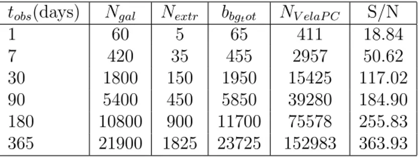
Vela pulsar is very bright object then we study the possibility to include the background and its influence. The diffuse γ-ray background can be modeled using two components: a Galactic diffuse component and an Extragalactic diffuse component. The Galactic diffuse emission is mainly due to interaction between cosmic rays and interstellar medium and has a distribution concentrated in the Galactic plane. The extragalactic component has a quite isotropic distribution and probably it is mainly due to the emission of faint unresolved extragalactic blazars.
We used simulations to study the number of photons detected by the LAT around the position of the simulated sources and we used it to estimated the Signal to Noise ratio. The Galactic diffuse emission intensity has been simulated using an emission model developed by the LAT Collaboration and based on GALPROP (Strong & Moskalenko, 1998; Strong et al., 2004). The spectrum of the galactic diffuse background is fairly complex since it is the result of several processes, including pion decay, bremsstrahlung and Compton scattering. The simulation uses intensities maps at 17 energies (∼ factor of 2 from 10 MeV to about 655 GeV), that are generated by GALPROP considering pion decay, Inverse Compton scattering and Bremsstrahlung. The total flux between 10 MeV and about 655 GeV is of about 10.58 ph m−2 s−1.
The extragalactic diffuse emission has been modeled as a power-law with spectral index of 2.1 and a total flux of Fextr=10.7 ph m−2s−1 between 20 MeV and 200 GeV.
We can write the signal to noise ratio is function of the observation time tobs:
S
N(tobs) =
stobs
pbgal∆Ωtobs+ bextr∆Ωtobs+ stobs
(9.1) Where s is the rate of photons from Vela, bgal is the rate of photons per solid angle of
the Galactic diffuse emission, bextr is the rate of detected photons per solid angle of the
extragalactic diffuse emission. Since we selected photons coming from a region within 3◦ from the simulated sources, ∆Ω is the correspondant the solid angle of the selected
sky region.
Since diffuse emission would have been different at the two locations of pulsar VelaPC and VelaOG, we used simulations to evaluate how many background photons are in
tobs(days) Ngal Nextr bbgtot NV elaP C S/N 1 60 5 65 411 18.84 7 420 35 455 2957 50.62 30 1800 150 1950 15425 117.02 90 5400 450 5850 39280 184.90 180 10800 900 11700 75578 255.83 365 21900 1825 23725 152983 363.93
Table 9.1: Evaluation of Signal to Noise ratio for Vela Polar Cap. The background photon number Ngal,Nextr and their total Ngal are evaluated on the basis of a single-day
background simulation. The number of photons from the source comes directly from the simulation.
tobs(days) Ngal Nextr bbgtot NV elaP C S/N
1 56 5 61 456 20.05 7 392 35 427 3200 53.13 30 1680 150 1830 16249 120.85 90 5040 450 5490 41017 190.20 180 10080 900 10980 79453 264.21 365 20440 1825 22265 160854 375.89
Table 9.2: Evaluation of Signal to Noise ratio for Vela Outer Gap. The background photon number Ngal,Nextr and their total Ngal are evaluated on the basis of a single-day
background simulation. The number of photons from the source comes directly from the simulation.
these region. We compute background for one day. Since GLAST orbital period, this means that in one day there is about 15 orbits, that guarantee an uniform exposure over the entire sky, then a simulation of 1 day give an good average of detected photons from the background.
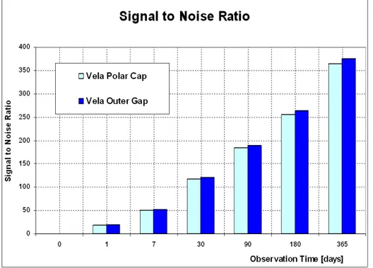
We evaluate the signal to noise ratio for different observation timescales and the results are reported in Tab. 9.1 and for Outer Gap in Tab. 9.2.
The various signal to noise ratios for both models are also displayed in Fig. 9.3. It is clear that already for 1 day the signal to noise ratio is about 20 and it is increasing with time, so we assume that we can neglect the background in our simulations.
We then prooceed to simulated only VelaPC and VelaOG for 1 year of simulated LAT observation with GLAST orbiting in scanning mode.
In order to evaluate the capability to measure spectrum of simulated sources with time the original 1-year simulation has been divided into smaller pieces, in order to obtain smaller observations, with respective lengths of 1 day, 1 week, 1 month, 3 months, 6 months and the original 1 year long observation.
The selection of region of the sky is very important since with real data it is important to reduce diffuse emission and pollution from other sources. Since LAT Point Spread Func-tion (PSF) is energy-dependent, it should be very useful to apply an energy-dependent selection on the acceptance angle.
Since Vela is very bright we found that an energy-independent acceptance radius can be also used. The LAT PSF at 100 MeV is little more than 3◦ and then we choose a
Figure 9.3: Signal to noise for both Vela Polar Cap and Vela Outer Gap for different observation times tobs with LAT operating in scanning mode.
from the location where the simulation source is places are accepted. The spectra have been then constructed and analyzed using XSpec v123
, and the total spectrum have been divided in 15 or 20 energy bins equally logarithmically spaced. In order to study the spectra with XSpec we adopt a model spectrum composed by a power law with exponential or super-exponential cutoff respectively for Polar Cap or Outer Gap Vela. Since the super-exponential cutoff is not implemented in the basic version of XSpec, we develop a simple spectral component with these characteristics and implement as user-defined model in XSpec.
9.3
Results
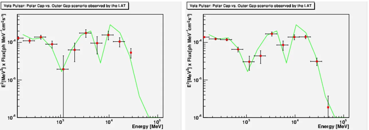
In order to do spectral analysis the spectral data have been binned in 15 bin equally spaced between 100 MeV and 300 GeV. We analyzed data on timescales of 1 day, 1 week, 1 month, 3 months, 6 months and 1 year. Fig. 9.4 and Fig. 9.5 show the reconstructed spectrum using the procedure described before. The normalization in the plots have been computed using XSpec, that consider the exposure and also the response matrix of the instrument. An important observation timescale is the full simulation of 1 year, whose result is displayed in Fig. 9.6 In order to establish how the difference between models varies with energy we decided to plot the theoretical difference between the fluxes for the two models and compare with the reconstructed spectra. We introduce
3
Figure 9.4: Reconstructed spectra of Vela Pulsar for Polar Cap model (light green) and Outer Gap model (dark blue). The lines represent the theoretical model, and the points the reconstructed spectrum. Left: Observation of 1 week in scanning mode. Right: Observation of 1 month in scanning mode.
Figure 9.5: Reconstructed spectra of Vela Pulsar for Polar Cap model (light green) and Outer Gap model (dark blue). The lines represent the theoretical model, and the points the reconstructed spectrum. Left: Observation of 3 months in scanning mode. Right: Observation of 6 months in scanning mode.
the quantitity FP C defined as:
FP C = E
2 dN
dEdtdS (9.2)
that indicate the square of the energy times the differential photon flux in ph cm−2 s−1
for Polar Cap Vela. This correspond to write the νlogFν useing the energy and represent
the output flux per unit of logarithmic energy. For Outer Gap we define in a similar way FOG.
The quantity DOG−P C = |FOG-FP C| can be used to show where the specrta of the two
models show the higher difference or distance.
These plots are useful to show where the maximum difference is, that could give a good hint to show which energy band select to better look for checking one or the other model. Fig. 9.7 The error of the quantity DOG−P C depends on both uncertanty on δFP C and
Energy [MeV] 3 10 104 105 ] -1 s -2 cm -1 ] x Flux[ph MeV 2 [MeV 2 E -6 10 -5 10 -4 10 -3 10
Polar Cap model prediction (Daugherty & Harding 1996). Polar Cap model, 1 yr LAT survey
Outer Gap model prediction (Romani 1996) Outer Cap model, 1 yr LAT survey EGRET data points (Thompson et al. 1999)
Vela Pulsar: Polar Cap vs. Outer Gap scenario observed by the LAT
Figure 9.6: Reconstructed spectra of Vela Pulsar for Polar Cap model (light green) and Outer Gap model (dark blue) for an observation time of 1 year. The lines represent the theoretical model, and the points the reconstructed spectrum. The black square points represent the EGRET data.
Figure 9.7: The quantity DOG−P C defined in the text that show how the difference between spectra vary with energy. The line show the theoretical prediction and the points represent reconstructed spectra from LAT simulations.Left: Observation of 3 months in scanning mode. Right: Observation of 1 year in scanning mode.
δFOG. Since these errors are independent, the error on the difference have been
com-puted by summing them in quadrature. The error δDOG−P C =pδF2
P C+ δF
2
OG. In this
way the errors shown for points in Fig. 9.7 have been computed. It is possible to see that the maximum of the theoretical difference is about at 10 GeV, then this is to be considered a good energy band, but before it has to be established the weight of the errors on this evaluation.
simu-lations in order to give where is the better energy band to choose in order to maximize the relative error in DOG−P C. At lower energy the flux estimate has lower uncertanty
but the difference itself is also very small. Viceversa at higher energies the difference will become more evident but the uncertanty increase due to lower statistics. Thanks to the quantity DOG−P C is it possible to estimate what is the best energy band to have
the relative error lower.
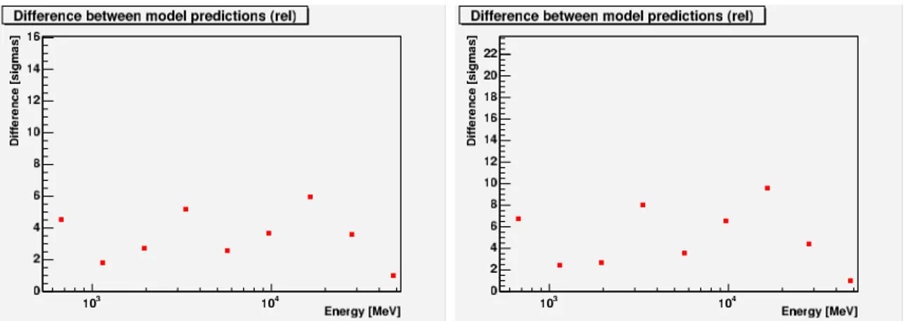
We computed and plot the difference in term of δDOG−P C and we labeled this as differ-ence between models expressed in terms of sigmas from the mean.
The quantity σOG−P C is then defined as:
σOG−P C = DOG−P C δDOG−P C = |FOG− FP C| pδF2 P C + δF 2 OG (9.3) Fig. 9.8 and Fig. 9.9 show the quantity σOG−P C for different time scales, respectively
Figure 9.8: Difference DOG−P C vs. energy evaluated in terms of sigma as explained in the text. Left: Observation of 1 month in scanning mode. Right: Observation of 3 months in scanning mode.
Figure 9.9: Difference DOG−P C vs. energy evaluated in terms of sigma as explained in the text. Left: Observation of 6 months in scanning mode. Right: Observation of 1 year in scanning mode.
of 1 month, 3 months, 6 months and 1 year.
There is a peak at about 3 GeV, in agreement with the Fig. 9.6, since at these ebergie the Polar Cap model exceeds the Outer Gap model. Altough at this energy the difference reach 8 sigma, we decided to neglect it since this bump does not appear to be a definite feature that distinguish Polar Cap from Outer Gap model. For example a small change in the power law at these energies could change this bump, while the high-energy cutoff appear to be a features that strongly characterize the Polar Cap emission from Outer Gap emission.
We are interested in studying high-energy cutoff and it is clearly visible that above 10 GeV σOG−P C increase up to the energy band centered in 9.6 GeV and then begin to decrease. This behaviour is in agreement with our evaluation that at higher energies the uncertanties in flux estimated become larger because of lower statistics. This lower statistics impact in the decrease if the denominator of the Eq. 9.3 then after about 10 GeV we expect that the difference between models begin to decrease. From these calculations in turns out that the best energy range where to look for maximum difference between model prediction is about 10 GeV.
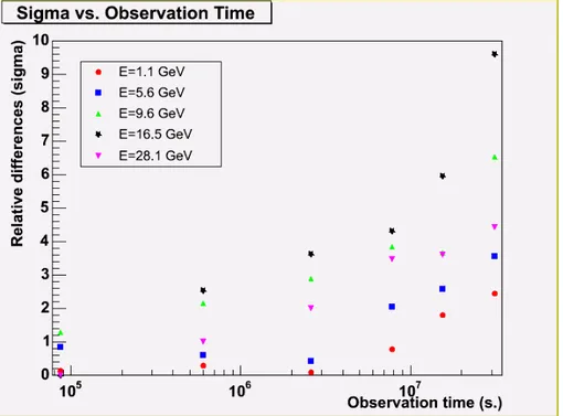
The results of plots in Fig. 9.8 and Fig. 9.9 can be summarized together with plots for lower observation times of 1 day and 1 week as in Fig. 9.10.
From this plot it can be seen that at lower energy (1.1 GeV and 5.5 GeV) the value of
Figure 9.10: Behaviour of σOG−P C with observation time. Some relevant energies are indicated with different markers.
σOG−P C is steady increasing but is always lower than 3, while the two enegies wher is
is increasingly better is 9.6 GeV and 16.5 GeV, where is is greater than 7σ for one year of observation.
As we expected at higher energies the value of σOG−P C increase not too much with time,
9.4
Discussion of the results
The LAT capabilities to distinguish between Polar Cap and Outer Gap model by looking at the high-energy cutoff is one of the most important item for better understanding physics of γ-ray emission in pulsars.
This enhanced capaility of studying spectra comes from the wider energy band of the LAT, that will allow the observation at energies above 30 GeV, a range that was not accessible to EGRET telescope. The higher effective area of the LAT will help to have much more photon statistics and then to measure with smaller errors fluxes at GeV energies.
A comparison between EGRET data and LAT simulated observation for 1 year has been presented in Fig. 9.6. The greater LAT energy range is clearly visible as well as the smaller error bars at few GeV that are expected to be very important to constrain one or the other model.
Results presented in previous Section show that it is possible to look for greater dif-ference between models by lookng at some particular energy band. The behaviour of
DOG−P C is useful to see where the difference is greater, but we need to know what are
the errors in flux estimates to correctly say what is the optimal energy band.
In order to do that simulations are very important to estimate what are the errors on flux. These are affected by energy resolution and by number of detected photons, then a knowledge of LAT Response Function is critical.
We decided to use as quantity to discriminate between models the σOG−P C, that is the reciprocal of the relative error. It give the difference between model expressed in terms of flux uncertanty, that we identified as sigmas.
It appear that the optimal range where to look for finding higher differences between model predictions is 10-16 GeV, since the maximum of the σOG−P C occurr for E=9.6
GeV and E=16.5 GeV. Above this energy statistics is very low and then σOG−P C become lower.
For observation time of the order of 1 year in scanning mode the discrimination between models is of 6σ for E=9.6 GeV and about 9.6σ for E=16.5 GeV.
From Fig. 9.10 it is possible to have a rough estimate on the smaller time required to have a distinction of 3σ and 5σ.
If the energy band selected is around 16.5 GeV we have that the minimum time t3σ ≃13
days to achieve a 3σ difference and t5σ ≃4 months for achieve a 5σ difference. These
val-ues are of course rough estimates and are dependent on the fact that these calculations have been made using simulations of LAT in scanning mode. LAT pointed observations will lead to similar estimates on shorter time scales.
The estimates and calculations made in this Section are based on some assumptions that must be considered in order to discuss also the possible limitation and extension to this work.
Regarding simulations, we decide to not simulate the dependence on the spectrum from the phase. Altough original theoretical models predict also phase-dependent spectra, our simulations have been built without considering them, since the main goal was to study the total flux witouth doing phase-resolved spectroscopy.
In the first Section an argument has been presented to show that the flux of background have been neglected for this study. The study of signal to noise ratio show clearly that for Vela it is always very high, so that the photons that contribute to the spectrum are