AAPP | Atti della Accademia Peloritana dei Pericolanti
Classe di Scienze Fisiche, Matematiche e Naturali
ISSN 1825-1242Vol. 91, Suppl. No. 1, A3 (2013)
PHASE-FIELD MODELING OF TRANSITION AND SEPARATION
PHENOMENA IN CONTINUUM THERMODYNAMICS
ALESSIABERTIaANDCLAUDIOGIORGIb∗
ABSTRACT. In the framework of continuum thermodynamics a new approach to phase transition and separation phenomena is developed by emphasizing their nonlocal charac-ter. The phase-field is regarded as an internal variable and the kinetic or evolution equation is viewed as a constitutive equation of rate type. The second law of thermodynamics is sat-isfied by virtue of an extra entropy flux which arises from its nonlocal formulation. Such an extra flux is proved to be nonvanishing inside the transition layer, only. Different choices of the state variables distinguish transition form separation models. The former case involves the gradients of the main fields up to the second order, whereas in the latter all gradients up to the fourth order are needed and the total mass of the phase-field is conserved. In both cases, necessary and sufficient restrictions on the constitutive equations are derived from thermodynamics. On this background, some applications to scalar-valued models are developed. A simple model of the temperature-induced first-order transition is derived in connection with a state space involving second-order gradients. Dynamical models of phase separation in a binary fluid mixture are discussed and the classical nonisothermal Cahn-Hilliard system is obtained as a special case of a fourth-gradient model.
“Nemo nisi per amicitiam cognoscitur” S. Agostino, De diversis quaestionibus, LXXXIII, LXXI, 5; PL, XL, 82
1. Introduction
A lot of theories have been recently developed in order to model either phase transition or phase separation phenomena which occur in many relevant processes in physics and engineering. In particular, the phase-field technique is one of the fastest growing areas in computational materials science and it has been applied to a large number of materials (see [19,37]). The goal of this contribution is to present the mathematical background of this method and give a detailed thermodynamical derivation of the phase-field equations for both transition and separation phenomena. The unifying point of view is to consider the phase-field as an internal (or hidden) variable.
When phase transition phenomena are considered, two distinct phases of the same sub-stance occur in a bounded, fixed domain Ω ⊂ R3with smooth boundary ∂Ω whose unit outward normal is denoted by n. Let x and t be the position vector and time, respectively. Each point x ∈ Ω is occupied by a single particle of the given substance, which may occur in two distinct forms, called phases. Each phase is labelled by a scalar value: 0 for the less
ordered phase, 1 for the most ordered one. In macroscopic modeling, an order parameter χ ∈ {0, 1} is attached to each particle, so that a phase transition may be described by a function χ(x, t) jumping from 0 to 1 and viceversa. In the simpler case, a sharp (but reg-ular) moving interface separates two regions occupied by the different phases. However, a highly uneven surface with possibly fractal Hausdorff dimension may occur in general conditions. In order to handle a more regular situation, we introduce a smooth scalar func-tion φ, the phase-field, whose values range continuously in the whole interval [0, 1] and whose evolution describes the phase transition. The function φ coincides with χ (namely, φ = 0 or φ = 1) in the bulk regions where the phases are pure, that is to say, outside a thin layer (all around the sharp interface) where the transition is localized. Inside this layer, which is named diffuse interface, a large but finite value of ∇φ occurs.
On the contrary, in phase-separation phenomena, each point x ∈ Ω is occupied by a mixture of two given substances, A and B, which are improperly called phases. Either in a binary metallic alloy or in a binary glassy fluid, phase separation describes the pro-cess by which the two components A and B of the mixture spontaneously separate and form domains pure in each component (see, for instance, [24]). From the mathematical point of view, it occurs as the asymptotic outcome of the evolution equation for the sin-gle scalar order parameter φ(x, t), which we can visualize as the average concentration around the position x of one of the components, φA and φB. Since φA + φB = 1, we have φA, φB ∈ [0, 1]. A perfect mixing between the two components corresponds to φA = φB = 1/2. Moreover, during phase separation material particles cannot change their “phase”, but they are simply allowed to migrate from a geometrical point to another close to it. As a consequence, the total measure (volume or mass) of each phase is con-served. That is to say, their integrals on the whole domain Ω does not change with time.
Once temperature is taken into account as an independent variable, phase-field theories are required to be “thermodynamically consistent”. That is to say, their evolution equa-tions must obey the First and Second Law of Thermodynamics. Such a requirement is the major difficulty in the formulation of nonisothermal models for temperature-induced phase transformations. In the 1990s a number of models consistent with Thermodynamics were proposed (see [21] and references therein). Subsequently, papers [5,15,16,17,18,33] contribute to enlighten the connection between the introduction of an entropy extra flux and the need to rescale the free energy by temperature. In those papers the authors assume the phase-field as an internal variable that accounts for nonlocal effects and justify the en-tropy extra flux as a consequence of this nonlocality (a close approach was early proposed by Maugin in [29]).
It is worth noting that across the diffuse interface the quantity φ needlessly agree with the concentration of one phase (the liquid phase, for instance, as in a scheme of fluid mixtures [33]). In the regions where one pure phase appears, the mass density ρ, as well as all other physical state variables, matches with the corresponding density of the material. Across the diffuse interface, on the contrary, ρ is described by an a-priori unknown function of φ, which results by a suitable superposition of the densities of the pure phases. Anyway, there is no need to identify the phase-field φ with any microscopic physical quantity. 1.1. Internal and state variables. The models presented here are schematic and limited to some aspects of the phenomenon which is involved. To this end, only few (scalar)
quantities are taken into account. These quantities, which include the phase-field, are called state variables: they characterize the initial conditions we need to prescribe in order to predict the evolution of the system. In the sequel, the set of all the state variables will be denoted by Σ. As well known, phase transitions are customarily considered as nonlocal phenomena. For instance, at the macroscopic level, a transition layer looks like a sharp interface whose motion is governed by a mean-curvature flow equation [39]. At the mesoscopic scale nonlocal spatial effects can be taken into account by a weakly nonlocal approach (see, for instance, [30,38]). In the framework of continuum thermodynamics, this approach leads to gradient-type models, where the dynamics at a point x is determined not only by the local values of the independent variables at the same point.
Henceforth, we assume that Σ is composed by some “primary” unknown fields (as well as density, temperature, ... , including the phase-field) and by their gradients up to some order greater than one. According to [31,32], the phase-field φ is viewed as an internal (or hidden) variable which varies across the diffuse interface according to a kinetic law of the rate type, namely
˙
φ = Φ(Σ) . (1)
When Φ depends on the gradients of φ up to the second order, this formulation is able to include the most common scalar phase-field theories based on the Ginzburg-Landau pioneering work [26]. If Σ involves the gradients of φ up to the fourth order, (1) is general enough to capture the well-known model of phase separation due to Cahn-Hilliard. In spite of this, some phase-change phenomena suggest a more complex internal behavior involving some (i.e., vector- and tensor-valued) hidden variable (see, for instance, [17,18, 6,7]). As well as any other constitutive law, the choice of Φ as a function of Σ is submitted to restrictions due to the Second Law of Thermodynamics, as depicted in §3 and §4.
In this paper we consider both first-order phase transition and phase separation in mul-tiphase compressible viscous fluids and fluid mixtures. In spite of the rather simple nature of the material, nonlocal spatial effects due to the phase transition/separation phenomena are taken into account by assuming that Σ at a point x depends on the local values of ρ, θ, φ and their spatial derivatives up to some order greater than one. Accordingly, the corresponding mathematical models maight be named higher-gradient models.
Concerning this appellation, however, a word of warning is in order: it refers to mod-els where some constitutive equation (typically, the phase-field kinetic equation) depends on higher-order gradients of the basic unknowns, but the free energy is independent of their spatial derivatives of order greater than one (see, for instance, § 3). Higher-gradient models should not be confused with higher-gradient theories. Indeed, the latter are well established in the literature and refers to a continuum thermodynamic description where the free energy depends on the first, second and higher-order gradients of the basic vari-ables. For instance, second gradient theories have been developed in mechanics for treating second-grade materials [20] and different phenomena as capillarity in fluids, liquid-vapor flows [23], plasticity and friction in granular materials [12]. In this concern, we quote [30], where a comparison between nonlocal theories and gradient-type theories is addressed. To our knowledge, few papers deal with higher-order gradient models and they are mostly devoted to theories involving internal variables (see [31,32]).
1.2. Plan of the paper. First, in § 2 we introduce balance and constitutive equations. In § 3 a suitable exploitation of the nonlocal form of the Clausius-Duhem inequality yields a general class of second-gradient models with internal variable and we construct a class of models describing phase-field transitions into a compressible fluid. The classical model of a first order transition (ice-water, for instance) is considered in § 3.2 as a special case. As scrutinized in § 4, a more general choice of the state variables, jointly with some exploita-tion of the Clausius-Duhem inequality, yields a larger class of models which are referred to as forth-gradient models with internal variable. All of them accounts for temperature, den-sity and velocity variations and are able to describe phase separation in binary compressible fluid mixtures. To this end, the phase-field φ is identified with the mass concentration of one of the components of the mixture. In particular, § 4.2 is devoted to obtain a nonisother-mal generalization of the Cahn-Hilliard system. Finally, some conclusions are drawn in § 5, where the advantages of this novel approach is discussed. The Appendix, at the end of the paper, collects some lengthly proofs.
2. Balance laws, entropy inequality and constitutive equations
Henceforth, we denote by symA and skwA the symmetrical and skew part of a tensor A, symA = 1 2A + A T , skwA = 1 2A − A T ,
where the symbol T stands for the transpose of a tensor, and by sphB and devB the spherical and deviatoric (or traceless) part of a symmetric tensor B,
sphB = 1
3(trB)I, devB = B − 1 3(trB)I, where trB = B · I. In particular, we define
Ω = skwL, D = symL, D◦= devD. (2)
Moreover, we use the superposed dot to denote the total time derivative, namely ˙
f (x, t) = ∂tf (x, t) + v(x, t) · ∇f (x, t).
According to continuum thermodynamics, the choice of the state variables for the specific model depends on the equations which are involved: the balance laws and the constitutive laws. We start by writing the balance equations of mass, linear momentum and energy in the eulerian form
˙
ρ + ρ∇ · v = 0 ρ ˙v = ∇ · T + ρb ρ ˙ε = T · L − ∇ · q + ρr
(3)
where v is the velocity of the particle, θ the absolute temperature, ρ the mass density, L = ∇v and ∇ = ∂x is the gradient operator. For further convenience, from (3)1 we deduce the equality
trD = ∇ · v = −ρ˙
ρ. (4)
The sources b and r are given function of x, t and represent the external body force and heat supply density, respectively. Finally, T is the Cauchy stress tensor, ε the internal
energy density, q the heat flux vector. All these quantities, jointly with the entropy density η, are prescribed as functions of the state variables by means of the following constitutive laws
T (x, t) = −ˆp(Σ(x, t))I + ˆS(Σ(x, t), L(x, t)) , q(x, t) = ˆq(Σ(x, t)) , (5) ε(x, t) = ε(Σ(x, t)) ,ˆ η(x, t) = ˆη(Σ(x, t)) , (6) where p = ˆp(Σ) denotes the pressure and I stands for the identity tensor. For further convenience, we let
ˆ
S(Σ, L) = ˆS0(Σ) + ˆSv(Σ, L)
where Sv = ˆS(Σ, L) is a symmetrical tensor which takes into account viscous effects and S0= ˆS(Σ) is the (deviatoric) extra-stress tensor due to phase interfaces. The fluid is named inviscid if Sv = 0. As usual, the resulting symmetry of the stress tensor T accounts for the balance of angular momentum.
The constitutive equation for the phase variable φ is given by the rate-type equation (1), namely
˙
φ = Φ(Σ).
We need now a nonlocal statement for the Second Law of Thermodynamics in order to account for the character of the phenomena involved. Let η be the entropy density and σ the entropy supply density.
Entropy Principle. For all fields ρ, θ, v, T , q, b, r which are compatible with the balance laws(3) and the constitutive laws (1) and (5)-(6), the following integral equality holds
d dt Ω ρ η dv = − ∂Ω q θ · n da + Ω ρσdv, (7)
whereσ = σ1+ σ2satisfies the conditions σ1=
r
θ, σ2≥ 0 , inΩ × R +.
We stress that this statement of the Second Law has a nonlocal nature since (7) is assumed to hold on the whole domain Ω, only (see, for instance, [22,34]). By applying the diver-gence theorem, we obtain
Ω ρ ˙η dv = − Ω ∇ ·q θ dv + Ω ρr θ dv + Ω ρσ2dv. This is equivalent to state the local entropy balance
ρ ˙η + ∇ ·q θ
−ρr
θ − ρσ2= −∇ · k, where k = k(x, t) is a regular field, called entropy extra flux, such that
Ω ∇ · kdv = ∂Ω k · nda = 0. As a consequence, inside Ω the entropy inequality (7) takes the form
ρ ˙η ≥ −∇ ·q θ + k
+ρr
where the entropy flux vector is redefined up to the extra contribution k. Henceforth, we assume that the entropy extra flux obeys the constitutive law
k = ˆk(Σ).
We denote by ψ = ψ(Σ) the Helmholtz free energy density, ˆ
ψ(Σ) = ˆε(Σ) − θ ˆη(Σ).
By differentiating this relation with respect to t and substituting (3)3and (8), we obtain the Clausius-Duhem inequality
− ρ( ˙ψ + η ˙θ) + T · D −1
θq · ∇θ + θ∇ · k ≥ 0. (9)
3. Second-gradient models for scalar phase changes
For the sake of simplicity, we first neglect third and higher order gradients and we consider the set
Σ = (σ, ∇σ, ∇∇σ).
where σ = (ρ, θ, φ). This second-order approximation is assumed throughout this section. It is needed in order that (1) entails the well-known Ginzburg-Landau equation and leads to what we call second-gradient model.
If the entropy extra flux k is assumed to vanish when no phase change occurs (cf. [3]), then the following result holds (see [5], Prop. 3.2, and also [15]). Its proof is summarized into the Appendix.
Proposition 3.1. Let the entropy extra flux k be homogeneous with respect to ˙φ, namely
k = 0 when φ = 0.˙ (10)
Then, constitutive functionsε, ˆˆ η, ˆT , ˆq, Φ, ˆk are compatible with the second law of Thermo-dynamics if ψ = ˆψ(ρ, θ, φ, ∇φ), (11) S0 = −ρ dev(∇φ ⊗ ∂∇φψ)ˆ skw(∇φ ⊗ ∂∇φψ) = 0,ˆ (12) ˆ p = ρ2∂ρψ +ˆ ρ 3∇φ · ∂∇φ ˆ ψ, η = −∂ˆ θψ,ˆ (13) ˆ k = 1 θρ ∂∇φ ˆ ψ Φ, Φ ∂∇φψ · n|ˆ ∂Ω= 0 (14)
Finally, the Clausius-Duhem inequality reduces to ∂φψ − ∇ · ∂ ∇φψ Φ −1 θ ˆ Sv· D + 1 θ2q · ∇θ ≤ 0.ˆ (15) where ψ = ρ ˆψ/θ is named “rescaled” Helmholtz free energy density (per unit volume).
By virtue of (14)1it is apparent that the entropy extra flux is non-zero only across the diffuse interface, where ∇φ ̸= 0, and vanishes when ˙φ = 0. This means that in the pure
phases the Clausius-Duhem inequality (9) assumes the standard form (see, for instance, [13])
−ρ( ˙ψ + η ˙θ) + T · D −1
θq · ∇θ ≥ 0.
Remark 3.2. As well-known (see, for instance, [34]), in the scheme of binary mixtures, the entropy extra flux is proportional to the relative velocity between both constituents. But this is not the point of view of this paper, since phases are not considered here as two distinct fluids. Accordingly, as pointed out in [33], in modeling phase transitions where mixtures are involved two terms occur into the entropy extra flux, one of which depends on the relative velocity and the other looks like (14)1.
In view of (15), it is quite natural to assume ˆ
q = −κ∇θ, tr ˆSv = ζ1trD, dev ˆSv = ζ2D◦, (16) Φ = −α∂φψ − ∇ · ∂ ∇φψ
, (17)
where κ, ζ1, ζ2, α are nonnegative functions of Σ. When newtonian fluids are concerned, ˆ
Sv= ℓ(ρ, θ)(trD)I + 2ζ(ρ, θ)D , ζ1= ℓ(ρ, θ) + 2
3ζ(ρ, θ) , ζ2= 2ζ(ρ, θ). (18) In particular, the fluid is inviscid provided that ℓ, ζ = 0. As apparent, equations (1) and (17) completely rule the evolution of φ so that the transition kinetics depends only on ψ,
˙
φ = −α∂φψ − ∇ · ∂ ∇φψ
. (19)
In addition, assuming that Φ ̸= 0 a.e. on ∂Ω, (14)2yields the natural boundary condition
∂∇φψ · n|ˆ ∂Ω= 0. (20)
Remark 3.3. During a process where mass density and temperature are uniform, namely ρ = ρ(t), θ = θ(t), the kinetic equation (19) takes the typical Ginzburg-Landau form
˙
φ = −α⋆[∂φψ − ∇ · ∂∇φψ] ,
where α⋆= αρ/θ and ψ is the usual Helmholtz free energy density (per unit mass). 3.1. Phase-field models for first-order transitions. In this subsection we consider some phase-field models for first-order transitions in a material (water, for instance) that in the liquid phase looks like an inviscid fluid. Namely, we assume that ζ1 = ζ2 = 0 in (16)2,3 and its constitutive properties are expressed by choosing
Γ = (ρ, θ, φ, ∇ρ, ∇θ, ∇φ, ∆ρ, ∆θ, ∆φ)
as the set of state variables. So far we know that, because of the thermodynamic restriction (11), the free energy ψ depends on Γ only through ρ, θ, φ and |∇φ|, but such dependence is arbitrary. For materials like as water, a general class of scalar-valued phase-field models is obtained by assuming that the free energy density ψ (per unit mass) have the additive form ˆ ψ(ρ, θ, φ, |∇φ|) = ˆψ1(ρ, θ, φ) + ˆψ2(θ, φ) + 1 2µ(ρ, θ, φ)|∇φ| 2. (21) The first term represents the stored mechanical energy. In connection with solid-liquid and liquid-vapor transitions, its expression involves the pressure function. The second
addendum represents the stored thermal energy and have to account for the thermodynamic condition
ˆ
ε = ˆψ − θ ∂θψ.ˆ (22)
The last term accounts for the interface energy, which is proportional to the width of the diffuse interface between two pure phases. The function µ is assumed to be positive valued, since ψ must attain a minimum at the homogeneous phases, i.e. when ∇φ = 0. In particular, if µ is assumed to be constant, we recover the customary quadratic dependence on ∇φ introduced by Cahn and Hilliard in [11] for isothermal processes (see also [8]). On the other hand, under non isothermal conditions it is more convenient to choose
µ(ρ, θ, φ) = µ0(ρ, φ)θ , µ0> 0.
Indeed, in this case the internal energy ˆε is independent of |∇φ| and (22) reads ˆ
ε = ˆψ1− θ ∂θψˆ1+ ˆψ2− θ ∂θψˆ2. (23) According to all these assumptions, thermodynamic restrictions (13) yield
η = −∂θψˆ1− ∂θψˆ2− 1 2µ0|∇φ| 2, p = ρˆ 2∂ ρψˆ1+ 1 2ρ θ ρ ∂ρµ0+ 2 3µ0 |∇φ|2. Therefore, in first-order phase transformations, as well as solid-liquid or liquid-vapor tran-sitions, the typical form of the kinetic boundary value problem (19)-(20) reads
˙ φ = −α ρ θ∂φ ˆ ψ1+ ˆψ2 + 1 2ρ ∂φµ0|∇φ| 2− ∇ · (ρµ 0∇φ) , ∇φ · n|∂Ω= 0.
If µ0 is a positive constant, the expression of the kinetic equation may be further sim-plified as follows ˙ φ = −αρ θ∂φ ˆ ψ1+ ˆψ2 − µ0(∇ρ · ∇φ + ρ∆φ) . (24)
On the other hand, when an inviscid fluid is considered, from (12)-(13) it follows ˆ T = −ρ2∂ρψˆ1I − µ0θρ∇φ ⊗ ∇φ, p = −ˆ 1 3tr ˆT = ρ 2∂ ρψˆ1+ 1 3µ0θρ|∇φ| 2 (25) and the motion equation (3)2reads
ρ ˙v = −∇(ρ2∂ρψˆ1) − µ0∇ · (θρ∇φ ⊗ ∇φ) + ρb .
Finally, the temperature evolution results from inserting the expression (23) into the energy balance equation (3)3and taking into account (25), namely
ρ( ˆψ1− θ ∂θψˆ1+ ˆψ2− θ ∂θψˆ2)·= −ρ2∂ρψˆ1∇ · v − µ0θρ∇φ ⊗ ∇φ · D + ∇ · (κ∇θ) + ρr . Letting ˆψ∗= ˆψ1+ ˆψ2, a straightforward calculation yields
ρ θ∂θ,θ2 ψˆ∗θ−ρ [∂˙ φψˆ∗−θ ∂θ,φ2 ψˆ∗] ˙φ = ρ2θ ∂θ,ρ2 ψˆ∗∇·v+µ0θρ∇φ⊗∇φ·D−∇·(κ∇θ)−ρ r. Atti Accad. Pelorit. Pericol. Cl. Sci. Fis. Mat. Nat., Vol. 91, Suppl. No. 1, A3 (2013) [21 pages]
3.2. A first order transition model. Let Π = ˆΠ(ρ, θ, φ, ∇φ) be any sufficiently smooth scalar function such that ∂∇φΠ · n|∂Ω= 0, and let
P =
Ω Π dx
be the related functional. As well known, its variational derivative leads to the Euler-Lagrange equation δφP = ∂φΠ − ∇ · ∂∇φΠ. If we denote by F = Ω ψ dx
the rescaled (Helmholtz) free energy functional (cf. [4,36]), the kinetic equation (19) takes the form
˙
φ = −αδφF . (26)
This result is in perfect agreement with [4] (see also [8]). In particular, the critical points of the functional F , which satisfy δφF = 0, are solutions of the stationary problem
Φ(Σ) = 0.
If δφF is assumed to measure the distance of the system from equilibrium, then −α δφF can be viewed as a generalized “elastic” force, whose action drives the evolution of φ by attracting the system toward the equilibrium. In addition, we notice that
d dtF (φ(t)) = Ω δφF ˙φdv + ∂Ω γ ˙φ∇φ · n da. The boundary condition n · ∇φ = 0 at ∂Ω and (26) imply that
d dtF (φ(t)) = − Ω αδφF 2 dv ≤ 0 whence F (φ(t)) decays in time.
Of course, peculiar properties of first-order phase transition at fixed temperature strongly depends on the choice of ˜ψ. For the sake of simplicity, we restrict our attention to uniform processes where the mass density is constant (ρ = 1 and ∇φ = 0) and we let
ψ = θ[3φ4− 4φ3+ u(θ)(3φ4− 8φ3+ 6φ2)], where u(θ) = θ/θc. Since
∂φψ(φ, θ) = θ{12φ(φ − 1)[(1 + u(θ))φ + 1]},
we conclude that φ = 0 and φ = 1 are equilibrium solutions (i.e., local minimizers of the free energy) whatever may be the value of θ. More precisely, if θ > θcφ = 0 is the global minimum and φ = 0 is stable. On the contrary, if θ < θc then ψ attains its global minimum in φ = 1 (see Fig.1). At the transition temperature, θ = θc, ψ assumes the classical double-well shape, so that both solutions are stable (i.e., absolute minima).
Substituting the expression of ψ into equation (24), we deduce that the evolution of the phase-field is governed by
˙
0
1
ϕ
ψ
Figure 1. The graph of the free energy at different temperatures: θ/θc > 1 (solid),θ/θc= 1 (dashed) andθ/θc< 1 (short-dashed).
4. Fourth-gradient models for scalar phase changes
Unfortunately, starting from (1) the second-gradient model is unable to recover the Cahn-Hilliard equation, which is a fourth-order (in space) differential equation. The aim of this subsection is to overcome this difficulty by introducing a fourth-gradient model. To this end, first, we consider a more general set of state variables,
Σ = (σ, ∇σ, ∇∇σ, ∇∇∇σ, ∇∇∇∇σ),
where σ = (ρ, θ, φ). In addition, we need to devise a more general thermodynamic ap-proach by performing a direct exploitation of the nonlocal entropy inequality.
Starting from (7) and the Entropy Principle, we obtain the nonlocal entropy inequality (cf. [22]) Ω ρ ˙η dv ≥ − Ω ∇ ·q θ dv + Ω ρr θ dv. (27)
Now, accounting for the definition of ψ, the l.h.s. can be rewritten as Ω ρ ˙η dv = Ω ρ θ ˙ ε − ˙ψ − η ˙θdv,
and, by virtue of (3)3, the nonlocal entropy inequality (27) takes the form Ω 1 θ −ρ( ˙ψ + η ˙θ) + T · D −1 θq · ∇θ dv ≥ 0, (28)
which represents the nonlocal Clausius-Duhem inequality. By means of a local approach, as well as the procedure exhibited into the Appendix, the thermodynamic restrictions (11)-(13) can be proven to hold true even in the more general setting considered here. Then, taking advantage of (11)-(13), inequality (28) reduces to the following form
Ω 1 θ 1 θq · ∇θ − ˆˆ Sv· D dv + ∂Ω Φ ∂∇φψ · n da + Ω Φ∂φψ − ∇ · (∂ ∇φψ)dv ≤ 0, Atti Accad. Pelorit. Pericol. Cl. Sci. Fis. Mat. Nat., Vol. 91, Suppl. No. 1, A3 (2013) [21 pages]
where ψ = ρ ˆψ/θ is the rescaled free energy density (per unit mass). In order to satisfy (28), it is sufficient to assume the separate inequalities
Ω 1 θ 1 θq · ∇θ − ˆˆ Sv· D dv ≤ 0, (29) Ω Φ∂φψ − ∇ · (∂ ∇φψ) dv + ∂Ω Φ ∂∇φψ · n da ≤ 0. (30) This is quite natural, in that (29) comes down to the classical (nonlocal) form of the reduced inequalitywhich holds true when no phase change occurs (Φ = ∇φ ≡ 0). In particular, condition (29) can be locally satisfied if ˆq and ˆS obey the constitutive relations (16).
Finally, we derive some expression of Φ and some boundary conditions which ensure the validity of (30) in its general nonlocal form. Henceforth, for ease in writing, we let
Ξ = ∂φψ − ∇ · (∂ ∇φψ).
Proposition 4.1. Inequality (30) is satisfied provided that Φ in (1) is given by
Φ = ν∇ · [m∇(ν Ξ)] − αΞ, (31)
where ν, m, α are suitable functions of Σ such that m and α are nonnegative, and the following boundary conditions jointly hold
m∇(νΞ) · n|∂Ω= 0 , ∂∇φψ · n| ∂Ω= 0. (32) Proof. By replacing (31) for Φ into the first integral of inequality (30), it follows
∂Ω [Φ ∂∇φψ + m ν Ξ∇(ν Ξ)] · n da − Ω m |∇(ν Ξ)|2dv − Ω α Ξ2dv ≤ 0. At this point, boundary conditions (32) lead to
Ω m |∇(ν Ξ)|2dv + Ω α Ξ2dv ≥ 0,
which is satisfied provided that m, α ≥ 0. □
In the general case, the phase-field evolution is ruled by the system ˙ φ = ν∇ ·m∇ν∂φψ − ∇ · (∂ ∇φψ) − α∂φψ − ∇ · (∂ ∇φψ), m∇ν∂φψ − ∇ · (∂ ∇φψ) · n|∂Ω= 0, ∂∇φψ · n| ∂Ω= 0. (33)
This phase-field model seems to be new in the literature. However, for special values of the arbitrary functions involved, we are able to recover the kinetic equations of both the nonconservedand the conserved phase-field (see, for instance [8]).
Remark 4.2. If m = 0 and α > 0, then (31) provides Φ = −αΞ and we recover from (1) and(32) the evolution system of the Allen-Cahn type, namely (cf. (19), (20) and [1,2])
˙
φ = −α∂φψ − ∇ · (∂ ∇φψ), ∂∇φψ · n| ∂Ω= 0.
On the other hand, if we let α = 0 and m > 0 we obtain the evolution system for a phase-field of the Cahn-Hilliard type, namely
˙ φ = ν ∇ · {m∇[ν (∂φψ − ∇ · (∂ ∇φψ))]}, ∇[ν(∂φψ − ∇ · (∂ ∇φψ))] · n| ∂Ω= 0, ∂∇φψ · n| ∂Ω= 0. (34)
wherem represents the mobility function and ν∂φψ −∇·(∂ ∇φψ) stands for the chemical potential.
Remark 4.3. Let ν and α be constant. Assuming that α = 0, from (34) we have d dt Ω φ dv = Ω ˙ φ dv = ν ∂Ω m ∇(ν Ξ) · n da = 0, and the total phase-field P =
Ωφ dv is conserved. Vice-versa, assuming that ˙P = 0 along all processes, from(33) we have
0 = Ω ˙ φ dv = −α Ω Ξ dx, so that we inferα = 0.
Remark 4.4. Let ν = 1/ρ and α be constant. Then M =
Ωρ φ dv, the total moment of the phase-field, is conserved if and only ifα = 0. Indeed, assuming that α = 0, from (3)1 and(34) we have d dt Ω ρ φ dv = Ω ρ ˙φ dv = ∂Ω m ∇(ν Ξ) · n da = 0. Vice-versa, assuming that ˙M = 0 along all processes, from (33) we have
0 = −α
Ω ρ Ξ dx and thenα = 0 follows.
The procedure we described here emphasizes a double benefit. First, the introduction of the entropy extra flux k is avoided. Second, a more general phase-field evolution equation is obtained, which is able to depict both phase transition and phase separation phenomena. In our opinion, this simple derivation enlightens the origin of the most celebrated phase-field models and highlights their deep connections with continuum thermodynamics. 4.1. Phase-field models for separation of a binary fluid mixture. In this subsection we consider a multiphase, compressible, viscous, binary fluid mixture. By paralleling [28], we adopt the basic approach of partial miscibility regularization developed therein, so that the resulting theory involve the possibility of mixing of the two fluids. Accordingly, the phase-field can be interpreted as describing the concentration of one component of the mixture. To this end, we introduce a realistic concentration field, φ(x, t), which evolves according to a suitable diffusion model coupled to the equations of fluid flow and heat conduction.
In particular, let consider a heterogeneous mixture of two fluids with mass concentra-tions φi= Mi/M , i = A, B. Here, MAand MBare the masses of the components A and B in the representative material volume V . Since M = MA+ MB, we have φA+ φB = 1
and φA, φB ∈ [0, 1]. Suppose that the two fluids move with different velocities vi and have different apparent densities ˜ρi= Mi/V . Then the equation of mass balance for each component can be written in the form,
˙˜
ρi+ ˜ρi∇ · vi= 0 , i = A, B.
If we introduce the mass-averaged velocity ρv = ˜ρAvA+ ˜ρBvB, where ρ = ˜ρA+ ˜ρB = M/V is the total density, then the mass balance equation (3)1holds true. It is worth noting that ρφi= ˜ρiso that
Ω
ρφidv = Mi, i = A, B. (35)
and each phase-field concentration is conserved in the sense of Remark 4.4. In addition, the actual mass densities ρi= Mi/Viare related to apparent mass densities through ˜ρi= γiρi where γi = Vi/V are the volumetric fractions which satisfy γA+ γB = 1. Henceforth the phase-field can be interpreted as describing the concentration of one of the components of the binary fluid, for instance φ = φA, so that φ ∈ [0, 1]. Nevertheless, different but equivalent choices are allowed, for instance by setting ϕ = φA− φB, so that ϕ = 2φ − 1 and ϕ ∈ [−1, 1].
In order to apply the procedure previously devised, we assume that constitutive prop-erties are expressed by choosing Σ as the set of state variables. Nevertheless, because of (11)1, the free energy ψ depends on Σ only through ρ, θ, φ and |∇φ|. Therefore, a quite general class of phase-field models for liquid materials is obtained by letting, as in §3,
ˆ ψ(ρ, θ, φ, |∇φ|) = ˆψ0(ρ, θ, φ) + 1 2µ0(ρ, φ)θ |∇φ| 2 .
where ˆψ0(ρ, θ, φ) = ˆψ1(ρ, θ, φ) + ˆψ2(θ, φ) (cf. (21)). As a consequence, the kinetic evolution system (34) takes the form
˙ φ = ν ∇ · {m∇[ν (ρ ∂φψˆ0/θ +12∂φµ0ρ |∇φ|2− ∇ · (µ0ρ ∇φ))]}, ∇[ν(∂φψ − ∇ · (µ 0ρ ∇φ))] · n|∂Ω= 0, µ0ρ ∇φ · n|∂Ω= 0. (36)
As apparent, this system can be written in the simpler form (1/ν) ˙φ = ∇ · J , J · n|∂Ω= 0, ∇φ · n|∂Ω= 0
where J = m∇[ν Ξ] is the diffusional flux vector and Ξ = ρ ∂φψˆ0/θ +12∂φµ0ρ |∇φ|2− ∇ · (µ0ρ ∇φ) is the generalized chemical potential.
Remark 4.5. Under isothermal condition, θ = θ0 = const., the kinetic equation (36)1 perfectly agrees with[28, eqn.(3.34)] provided that ν = 1/ρ and µ0= const., namely
ρ ˙φ = ∇ · {ν0∇[∂φψˆ0− ε0/ρ∇ · (ρ ∇φ)]}, ν0= m/θ0, ε0= µ0θ0. If this is the case, the phase-fieldφ is conserved in the sense of Remark 4.4. If we assume both isothermal and isochoric conditions, that isθ = θ0andρ = ρ0, the kinetic equation
(36)1reduces to the standard Cahn-Hilliard equation provided thatν and µ0are constant, ˙
φ = ν0∆[∂φψˆ0− ε0∆φ], ν0= m/θ0ρ0, ε0= µ0θ0. and the phase-fieldφ is conserved in the sense of Remark 4.3.
According to thermodynamic restrictions (13) and constitutive assumptions (5)1, (16) and (18)
ˆ
T = −ρ2∂
ρψˆ0(ρ, θ, φ) − ℓ(ρ, θ)trDI + 2ζ(ρ, θ)D − µ0(ρ, φ)θρ ∇φ ⊗ ∇φ , so that the customary splitting of this tensor between its spherical and deviatoric part yields
ˆ T = − ρ2∂ρψˆ0+ 1 3µ0θρ |∇φ| 2 −ℓ +2 3ζ trD I + 2ζD◦− µ0θρ dev(∇φ ⊗ ∇φ). Then, from the motion equation (3)2we have
ρ ˙v = −∇(ρ2∂ρψˆ0) + ∇ · [ζ(∇v + ∇vT) − µ0θρ∇φ ⊗ ∇φ] + ∇(ℓ ∇ · v) + ρb . It is worth noting that under isothermal condition (θ = const.) this equation perfectly agrees with [28, eqn.(3.34)]. Finally, from the heat equation (3)3we obtain
ρ c ˙θ + ρ λ ˙φ = ∇ · (κ∇θ) + ρ r − ρ2θ ∂θ,ρ2 ψˆ0∇ · v
− µ0θρ∇φ ⊗ ∇φ · D + (ℓ + 2ζ/3)(∇ · v)2+ 2ζ(D◦)2.
where c = −θ∂θ,θ2 ψˆ0represents the specific heat per unit mass and λ = ∂φψˆ0− θ ∂θ,φ2 ψˆ0. Summarizing previous results, the thermodynamics of a phase separation process is ruled by the following closed system of equations
˙ ρ + ρ ∇ · v = 0, ρ ˙v + ∇(ρ2∂ ρψˆ0) − ∇·[ζ(∇v + ∇vT) − µ0θρ∇φ ⊗ ∇φ] − ∇(ℓ ∇ · v) = ρb, ˙ φ = ν ∇ · {m∇[ν (ρ ∂φψˆ0/θ +12∂φµ0ρ |∇φ|2− ∇ · (µ0ρ ∇φ))]}, ρ c ˙θ + ρ λ ˙φ = ∇ · (κ∇θ) + ρ r − ρ2θ ∂2 θ,ρψˆ0∇ · v − µ0θρ∇φ ⊗ ∇φ · D + (ℓ + 2ζ/3)(∇ · v)2+ 2ζ(D◦)2. (37)
Boundary conditions are obtained by collecting (36), the customary no-slip condition for v and the Robin boundary condition for θ,
v|∂Ω= 0 ∇[ν (ρ ∂φψˆ0/θ +12∂φµ0ρ |∇φ|2− ∇ · (µ0ρ ∇φ))] · n|∂Ω= 0, µ0ρ ∇φ · n|∂Ω= 0, aθ + b∇θ · n|∂Ω= g.
A special form of (37) is achieved by assuming ν = 1/ρ and µ0 = constant. It can be referred as Fourier-Navier-Stokes-Cahn-Hilliard (FNSCH) system, and reads
˙ ρ + ρ ∇ · v = 0 ρ ˙v + ∇(ρ2∂ ρψˆ0) − ∇ · [ζ(∇v + ∇vT) − µ0θρ∇φ ⊗ ∇φ] − ∇(ℓ ∇ · v)?ρb, ρ ˙φ = ∇ · {m∇[(1/θ)∂φψˆ0− (µ0/ρ)∇ · (ρ ∇φ)]}, ρ c ˙θ + ρ λ ˙φ = ∇ · (κ∇θ) + ρ r − ρ2θ ∂2 θ,ρψˆ0∇ · v − µ0θρ∇φ ⊗ ∇φ · D + (ℓ + 2ζ/3)(∇ · v)2+ 2ζ(D◦)2.
equipped with the following set of boundary conditions v|∂Ω= 0 ∇[(1/θ)∂φψˆ0− (µ0/ρ)∇ · (ρ ∇φ)] · n|∂Ω= 0, ∇φ · n|∂Ω= 0, aθ + b∇θ · n|∂Ω= g.
As previously remarked, this system represents the natural generalization to non isothermal processes of the Navier-Stokes-Cahn-Hilliard (NSCH) system derived in [28].
4.2. The Cahn–Hilliard equation. Chemical thermodynamics of immiscible fluid mix-tures predicts that at low temperamix-tures there is a limited miscibility between the fluid com-ponents [14,27]. For sake of simplicity, we restrict our attention to processes where the total mass density is constant. Then, letting ρ = 1 and φ = φA, the partial miscibility is characterized by equilibrium concentrations φ2 ≈ 1 (A–rich mixture) and φ1 ≈ 0 (B– rich mixture, since φB ≈ 1). As the temperature increases, equilibrium concentrations approach each other and eventually coincide so that the mixture miscibility gap, φ2− φ1, vanishes at a critical temperature θc. Above the critical temperature, the system exhibits a continuous sequence of molecular mixtures (solutions) and the fluids are considered to be completely miscible. If we confine our attention to homogeneous and incompressible processes, the particular model of mixing at a given temperature is formulated by assum-ing that the specific free energy density is convex when fluids are miscible and nonconvex when they are partially miscible.
The Cahn-Hilliard equation is the simpler mathematical model which is able to describe all these characteristic items of spinodal decomposition [10,25]. Such a model accounts for conserved dynamics, in which the integral of φ on Ω is constant in time (see [8], p. 166), stems from the mass balance equation
˙
φ = −∇ · j and the generalized Fick’s law
j = − ˆK(φ)∇G
where ˆK is a positive parameter, which represents the diffusive mobility, j can be viewed as the driving force of the phase separation and the chemical potential G is given by
G = δφF , where the free energy functional F has the form
F (φ) = Ω ψ0(φ, θ) + 1 2µ0(φ, θ)|∇φ| 2dv, ψ0(φ, θ) = 1 θψ0(φ, θ). In the simple case that µ0and ˆK are constants it follows that φ is governed by
˙
φ = ˆK∆(∂φψ0− µ0∆φ).
which is called Cahn-Hilliard equation. Assuming the boundary conditions n · ∇φ = 0, n · ∇δφψ0= 0, at ∂Ω,
Of course, the spinodal decomposition at fixed temperature strongly depends on ψ0. For instance, letting φ = φA, we can choose a fourth-order polynomial (see [28, eqn.(6.20)])
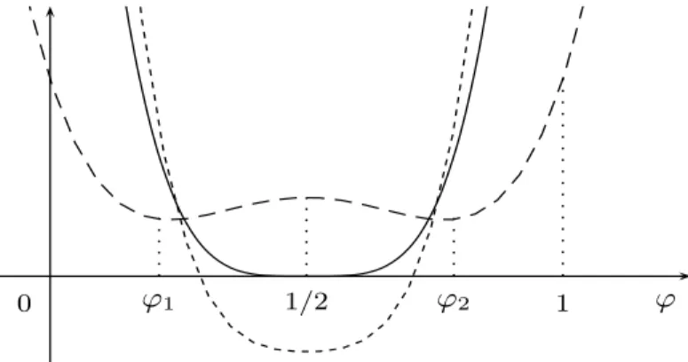
ψ0(φ, θ) = θ[(2φ − 1)4− 2v(θ)(2φ − 1)2+ v(θ)], where v(θ) = (θc− θ)/θc. As a consequence,
∂φψ0(φ, θ) = 8θ(2φ − 1)[(2φ − 1)2− v(θ)] , ∂2φφψ0(φ, θ) = 16θ[3(2φ − 1)2− v(θ)]. When θ > θcwe have v(θ) < 0, so that ∂φψ0vanishes at φ = 1/2 and ∂φφ2 ψ0is positive for all values of φ. On the contrary, when θ ≤ θcthen v(θ) ≥ 0, and we have
∂φψ0= 0 at φ0= 1 2, φ1= 1 −v(θ) 2 , φ2= 1 +v(θ) 2 , ∂φφ2 ψ0= 0 at φ∗1= 1 −v(θ)/3 2 , φ ∗ 2= 1 +v(θ)/3 2
Accordingly, as θ ∈ (0, θc) the function ψ0(φ, θ) has two local minima at φ1(θ), φ2(θ) and a local maximum at φ0. If θ ≥ θcthen ψ0has only a minimum at φ = 1/2 (see Fig. 2).
1 1/2
0
ϕ
1ϕ
2ϕ
Figure 2. The free energyψ0 at temperaturesθ > θc(short-dashed),θ = θc (solid) andθ < θc(dashed).
The isobaric phase diagram generated by representing φ = φ1(θ) and φ = φ2(θ) in the (φ, θ)-plane (temperature vs composition) is named coexistence curve. The area below this curve is often referred as miscibility gap. In the same plane, the chemical spinodalis defined by the locus of the points of inflexion, φ = φ∗1(θ) and φ = φ∗2(θ). Any homogeneous solution cooled into the miscibility gap tends to decompose into A–rich and B–rich regions with a net reduction in the free energy. In particular, homogeneous solutions which are cooled within the chemical spinodal become unstable to infinitesimal perturbations in the chemical composition. Om the contrary, if a homogeneous solution is cooled into the region between the chemical spinodal and the coexistence curve, then large composition fluctuations are needed before phase separation can occur; this happens by a process known as nucleation and growth (see Fig. 3).
1 1/2 0
θ
cθ
ϕ
ϕ
1ϕ
∗1ϕ
∗2ϕ
2Figure 3. In the upper part of the picture, the graph of the free energyψ0(φ) at constant pressure and temperatureθ < θc(solid). In the lower part, the graphs of the coexistence curve (dashed) and the chemical spinodal (short-dashed) in the(φ, θ)-plane.
5. Conclusions
This paper provides a description of nonisothermal phase transitions and phase separa-tions through a phase-field model. The approach is based on a general evolution equation (33) for the phase-field φ which is viewed as an internal variable. Owing to the intrinsic nonlocality of the phase-field model, the constitutive equations involve, among others, a dependence on the gradient ∇φ and on the Laplacian ∆φ. Accordingly, the thermody-namic framework consists of the standard balance law of continuum physics (no internal structure), but the second law is stated in the form of a modified Clausius-Duhem inequal-ity where an extra flux of entropy, k, occurs. Compatibilinequal-ity with Thermodynamics is meant as the identical validity of the second law along any admissible process.
In simple models of continuum physics the entropy extra flux k vanishes in the bulk. On the contrary, here k is nonzero and its occurrence is related to the dependence of the free energy on ∇φ through the interface energy term. This in turn is consistent with the feature that nonlocal theories result in k ̸= 0. The constitutive equation (13)4for k is also consistent with the observation, made in different approaches (cf. [3,35]), that the fluxes are linear in ˙φ. The whole scheme is found to be compatible with thermodynamics, subject to appropriate restrictions on the constitutive relations and on the evolution equation. The natural condition (13)4makes the Clausius-Duhem inequality to hold and shows that the phase-field evolution is driven by the quantity Φ in (17). In addition, this makes it apparent why the approach through the rescaled functional provides the correct equations in non-isothermal conditions.
The main novelty of this approach is that the phase-field φ is regarded as an internal variable and that the corresponding evolution equation, governed by Φ, is deduced by means of thermodynamic arguments. The scheme is quite general and can be applied to both “non-conserved” and “conserved” phase-field models as documented in § 3.2 and § 4.2 by some applications.
6. Appendix
Proof of proposition 3.1
The free energy density ˆψ is a function of
Σ = (ρ, θ, φ, ∇ρ, ∇θ, ∇φ, ∇∇ρ, ∇∇θ, ∇∇φ).
Thus, by evaluating the time derivative of ˆψ and substituting into (9), we obtain −ρ∂ρψ ˙ˆρ + (∂θψ + η) ˙ˆ θ + ∂φψ ˙ˆφ + ∂∇ρψ ·ˆ ∇ρ + ∂˙ ∇θψ ·ˆ ∇θ˙ +∂∇φψ ·ˆ ∇φ + ∂˙ ∇∇ρψˆ∇∇ρ + ∂˙ ∇∇θψˆ∇∇θ + ∂˙ ∇∇φψˆ∇∇φ˙ −p ∇ · v + S0· D◦+ Sv· D −
1
θq · ∇θ + θ∇ · k ≥ 0. (38) On account of (1), one can easily check
˙
∇φ = ∇ ˙φ − LT∇φ = ∇Φ − LT∇φ, ∂∇φψ · Lˆ T∇φ = (∇φ ⊗ ∂∇φψ) · L.ˆ Accordingly, substitution of (1), (2) and (4) into (38) leads to
p ρ− ρ ∂ρ ˆ ψ −1 3∇φ · ∂∇φ ˆ ψ ˙ ρ − ρ(∂θψ + η) ˙ˆ θ + ∂φψ Φ + ∂ˆ ∇ρψ ·ˆ ∇ρ˙ +∂∇θψ ·ˆ ∇θ + ∂˙ ∇φψ · ∇Φ + ∂ˆ ∇∇ρψˆ∇∇ρ + ∂˙ ∇∇θψˆ∇∇θ + ∂˙ ∇∇φψˆ∇∇φ˙ +θ∇ · k + [S0+ ρ dev(∇φ ⊗ ∂∇φψ)] · Dˆ ◦+ Sv· D + ρ (∇φ ⊗ ∂∇φψ) · Ωˆ −1 θq · ∇θ ≥ 0.
By virtue of the arbitrariness of ˙ρ, ˙θ, D◦,∇ρ, ˙˙ ∇θ, ∇D◦,∇∇ρ,˙ ∇∇θ, Ω for any fixed˙ value of ρ, θ, ∇ρ, ∇θ, ∇∇ρ, ∇∇θ at (x, t) ∈ Ω, we obtain ∂θψ = −η,ˆ ∂ρψ =ˆ p ρ2 − 1 3ρ∇φ · ∂∇φ ˆ ψ, ∂∇ρψ = ∂ˆ ∇θψ = 0 ,ˆ ∂∇∇ρψ = ∂ˆ ∇∇θψ = 0 ,ˆ (39) skw(∇φ ⊗ ∂∇φψ) = 0,ˆ S0= −ρ dev(∇φ ⊗ ∂∇φψ).ˆ
Furthermore, the nontrivial dependence of Φ on ∇φ guarantees that even∇∇φ is arbitrary.˙ This can be proved by standard arguments and implies the further condition
∂∇∇φψ = 0.ˆ (40)
As a consequence of (39)-(40), we have
ψ = ˆψ(ρ, θ, φ, ∇φ) (41)
and the Clausius-Duhem inequality (38) reduces to − ρ∂φψ Φ − ρ∂ˆ ∇φψ · ∇Φ + Sˆ v· D −
1
θq · ∇θ + θ∇ · k ≥ 0. (42) Atti Accad. Pelorit. Pericol. Cl. Sci. Fis. Mat. Nat., Vol. 91, Suppl. No. 1, A3 (2013) [21 pages]
Since both k and Φ are assumed to be functions of Σ, by evaluating ∇ · k and ∇Φ (42) takes the form
−ρ∂φψΦ + (θ∂ˆ ρk − ρ∂∇φψ ∂ˆ ρΦ) · ∇ρ + θ∂θk − 1 θq − ρ∂∇φ ˆ ψ ∂θΦ · ∇θ +(θ∂φk − ρ∂∇φψ∂ˆ φΦ) · ∇φ + {θ∂D◦k − ρ∂∇φψ ⊗ ∂ˆ D◦Φ} · ∇D◦ +{θ∂∇ρk − ρ∂∇φψ ⊗ ∂ˆ ∇ρΦ} · ∇∇ρ + {θ∂∇θk − ρ∂∇φψ ⊗ ∂ˆ ∇θΦ} · ∇∇θ +(θ∂∇φk − ρ∂∇φψ ⊗ ∂ˆ ∇φΦ) · ∇∇φ + {θ∂∇D◦k − ρ∂∇φψ ⊗ ∂ˆ ∇D◦Φ} · ∇∇D◦ +{θ∂∇∇ρk − ρ∂∇φψ ⊗ ∂ˆ ∇∇ρΦ} · ∇∇∇ρ +{θ∂∇∇θk − ρ∂∇φψ ⊗ ∂ˆ ∇∇θΦ} · ∇∇∇θ +{θ∂∇∇φk − ρ∂∇φψ ⊗ ∂ˆ ∇∇φΦ} · ∇∇∇φ + Sv· D ≥ 0. (43) Taking advantage of (41), we can express all terms into the curly brackets as partial deriva-tives of the quantity θk − ρ∂∇φψ Φ. Then, from the arbitrariness of derivatives ∇∇Dˆ ◦, ∇∇∇ρ, ∇∇∇θ, ∇∇∇φ, which are all independent of Σ, it follows that
∂∇D◦(θk − ρ∂∇φψ Φ) = 0,ˆ ∂∇∇ρ(θk − ρ∂∇φψ Φ) = 0,ˆ
∂∇∇θ(θk − ρ∂∇φψ Φ) = 0,ˆ ∂∇∇φ(θk − ρ∂∇φψ Φ) = 0,ˆ
(44) and inequality (43) reduces to
−ρ∂φψΦ + (θ∂ˆ ρk − ρ∂∇φψ ∂ˆ ρΦ) · ∇ρ + θ∂θk − 1 θq − ρ∂∇φ ˆ ψ ∂θΦ · ∇θ +(θ∂φk − ρ∂∇φψ∂ˆ φΦ) · ∇φ + ∂D◦{θk − ρ∂∇φψ Φ} · ∇Dˆ ◦ +∂∇ρ{θk − ρ∂∇φψ Φ} · ∇∇ρ + ∂ˆ ∇θ{θk − ρ∂∇φψΦ} · ∇∇θˆ +(θ∂∇φk − ρ∂∇φψ ⊗ ∂ˆ ∇φΦ) · ∇∇φ + Sv· D ≥ 0,
which cannot be further reduced by means of standard arguments.
To overcome this problem, we adopt here a different approach, first devised in [18] and inspired to [4]. It is based on the assumption (10) and allows us to scrutinize (42) in a very simple way. Firstly we show that by virtue of (10) the entropy extra flux is given by
k(Σ) = 1 θρ ∂∇φ ˆ ψ ˙φ =1 θρ ∂∇φ ˆ ψ Φ. (45)
namely, we show that k is uniquely determined from ˆψ and Φ. Indeed, from (44) it follows that
θk − ρ∂∇φψ Φˆ
can be represented as an arbitrary function h = ˆh(ρ, θ, φ, D◦, ∇ρ, ∇θ, ∇φ). As a conse-quence, the entropy extra flux k has to satisfy
θk = ρ∂∇φψ ˙ˆφ + h. (46)
Finally, substitution of (45) into (42) leads to −ρ∂φψ Φ + Sˆ v· D − 1 θq · ∇θ + θ∇ · ρ θ∂∇φ ˆ ψΦ ≥ 0
and (15) is proved by means of straightforward manipulations. □ References
[1] S.M. Allen and J.W. Cahn, “A microscopic theory for domain wall motion and its experimental verification in Fe-Al alloy domain growth kinetics”, J. Phys. (Paris) Colloq. C 7 38, 51–54 (1977).
[2] S.M. Allen and J.W. Cahn, “A macroscopic theory for antiphase boundary motion and its application to antiphase domain coarsening”, Acta. Metal. 27, 1085–1095 (1979).
[3] H.W. Alt and I. Pawlow, “A mathematical model of dynamics of non-isothermal phase separation”, Phys. D59, 389–416 (1992).
[4] H.W. Alt and I. Pawlow, “On the entropy principle of phase transition models with a conserved parameter”, Adv. Math. Sci. Appl.6, 291–376 (1996).
[5] A. Berti and C. Giorgi, “A phase-field model for liquid-vapor transitions”, J. Non-Equilibrium Therm., 34, 219–247 (2009).
[6] V. Berti, M. Fabrizio and C. Giorgi, “Well-posedness for solid-liquid phase transitions with a fourth-order nonlinearity”, Physica D 236,13-21 (2007).
[7] V. Berti, M. Fabrizio and C. Giorgi, “A three-dimensional phase transition model in ferro-magnetism: exis-tence and uniqueness”, J. Math. Anal. Appl. 355, 661-674 (2009).
[8] M. Brokate and J. Sprekels, Hysteresis and phase transitions (Springer, New York, 1996).
[9] G. Caginalp, “An analysis of a phase-field model of a free boundary”, Arch. Rational Mech. Anal. 92, 205–245 (1986).
[10] J.W. Cahn, “Spinodal Decomposition”, 1967 Institute of Metals Lecture, Trans. Met. Soc. AIME, 242, 166–180 (1968).
[11] J.W. Cahn and J.E. Hilliard, “Free energy of a nonuniform system I. Interfacial energy”, J. Chem. Phys. 28, 258–267 (1958).
[12] C.S. Chang and J. Gao, “Second-gradient constitutive theory for granular material with random packing structure”, Internat. J. Solids Structures 32, 2279–2293 (1995).
[13] B.D. Coleman and W. Noll, “The thermodynamics of elastic materials with heat conduction and viscosity”, Arch. Rational Mech. Anal.13, 167–178 (1963).
[14] R.T. DeHoff, Thermodynamics in materials science (McGraw Hill, New york, 1993).
[15] M. Fabrizio, C. Giorgi and A. Morro, “A Thermodynamic approach to non-isotermal phase-field evolution in continuum physics”, Phys. D 214, 144–156 (2006).
[16] M. Fabrizio, C. Giorgi and A. Morro, “A continuum theory for first-order phase transitions based on the balance of structure order”, Math. Methods Appl. Sci. 31, 627-653 (2008).
[17] M. Fabrizio, C. Giorgi and A. Morro, “Phase transition in ferromagnetism”, Internat. J. Engrg. Sci. 47, 821–839 (2009).
[18] M. Fabrizio, C. Giorgi and A. Morro, “Isotropic-nematic phase transitions in liquid crystals”, Discrete Contin. Dyn. Syst. Ser. S4, 565–579 (2011).
[19] M. Fr´emond, Non-Smooth Thermomechanics (Springer, New york, 2001).
[20] E. Fried and M.E. Gurtin, “Tractions, Balances, and Boundary Conditions for Nonsimple Materials with Application to Liquid Flow at Small-Length Scales”, Arch. Rational Mech. Anal. 182, 513–554 (2006). [21] C. Giorgi, “Continuum thermodynamics and phase-field models”, Milan J. Math. 77, 67–100 (2009). [22] A.E. Green and N. Laws, “On a global entropy production inequality”, Quart. J. Mech. Appl. Math. 25,
1–11 (1972).
[23] D. Jamet, O. Lebaigue, N. Coutris and J.M. Delhaye, “The second gradient theory: a tool for the direct numerical simulation of liquid-vapor flows with phase-change”, Nuclear Engineering and Design 204, 155–166 (2001).
[24] R. A. L. Jones, Soft condensed matter (Oxford University Press, New York, 2002).
[25] J.E. Hilliard, “Spinodal Decomposition”, in Phase Transformations; H.I. Aaronson Ed. (American Society of Metals, Metals Park, 1970), p. 497.
[26] L.D. Landau and V.L. Ginzburg, “On the theory of superconductivity”, in Collected papers of L.D. Landau; D. ter Haar Ed. (Pergamon Press, Oxford, 1965).
[27] L.D. Landau and E.M. Lifshitz, Statistical physics (Pergamon Press, Oxford, 1958).
[28] J. Lowengrub and L. Truskinovsky, “Quasi-incompressible Cahn–Hilliard fluids and topological transi-tions”, Proc. R. Soc. Lond. A 454, 2617–2654 (1998).
[29] G.A. Maugin, The Thermomechanics of Nonlinear Irreversible Behaviors. An Introduction (World Scien-tific, Singapore, 1999).
[30] G.A. Maugin, “Nonlocal theories or gradient-type theories: a matter of convenience?”, Arch. Mech. 31, 15–26 (1979).
[31] G.A. Maugin and W. Muschik, “Thermodynamics with internal variables. Part I. General concepts”, J. Non-Equilibrium Therm.19, 217–249 (1994).
[32] G.A. Maugin and W. Muschik, “Thermodynamics with internal variables. Part II. Applications”, J. Non-Equilibrium Therm.19, 250–289 (1994).
[33] A. Morro, “A phase-field approach to non-isothermal transitions”, Math. Comput. Modelling 48, 621–633 (2008).
[34] I. M¨uller, Thermodynamics (Pitman, Boston, 1985).
[35] O. Penrose and P.C. Fife, “Thermodynamically consistent models of phase-field type for the kinetics of phase transitions”, Phys. D 43, 44–62 (1990).
[36] O. Penrose and P.C. Fife, “On the relation between the standard phase-field model and a ‘thermodynami-cally consistent’ phase-field model”, Phys. D 69, 107–113 (1993).
[37] I. Singer-Loginova and H.M. Singer, “The phase-field technique for modeling multiphase materials”, Rep. Prog. Phys.71, 106501–106533 (2008).
[38] P. V´an, “Weakly nonlocal irreversible thermodynamics”, Ann. Phys. (8) 12, 146–173 (2003).
[39] A. Visintin, “Introduction to Stefan-Type Problems”, in: Handbook of Differential Equations: Evolutionary Equations, C.M. Dafermos, M. Pokorny, Eds. (North-Holland Amsterdam2008); Vol. 4, pp. 377–484.
a Universit`a Telematica e-Campus
Facolt`a di Ingegneria Via Isimbardi 10
22060 Novedrate (CO), Italy
b Universit`a degli Studi di Brescia
Dipartimento di Matematica Via Valotti 9
25133 Brescia, Italy
∗ Email: [email protected]
Article contributed to the Festschrift volume in honour of Giuseppe Grioli on the occasion of his 100th birthday.
Received 5 November 2012; published online 29 January 2013
© 2013 by the Author(s); licensee Accademia Peloritana dei Pericolanti, Messina, Italy. This article is an open access article, licensed under aCreative Commons Attribution 3.0 Unported License.