7. GEOMETRIC ACCURACY 7.1 Introduction

7.

GEOMETRIC ACCURACY

7.1

Introduction

Accuracy of machined components is one of the most critical considerations for any manufacturer, as mentioned in Chapter 2. From the literature it is known that the accuracy of the products depends above all on the accuracy of the machine. For that reason after the evaluation of the dynamic accuracy, done in Chapter 6, it seems opportune to evaluate afterwards the geometric performance of the machine.

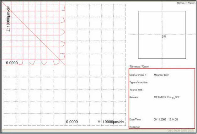
Fig. 7.1- Heidenhain test

It has been said in Chapter 6 that there was an opportunity to make some measurements on the micro-milling setup with the Heidenhain KGM. Besides the previously explained circular test another test has been conducted: the stages have been moved on a particular path (Fig. 7.1) during which the real path has been collected.

The path is a cross of vertical and horizontal lines which the stages have been moved on. Every division of the screen represents 10mm of length.

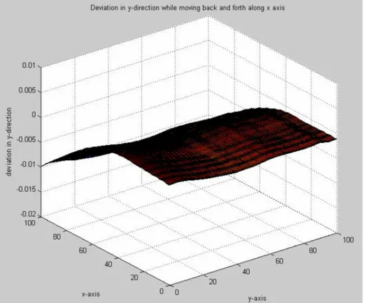
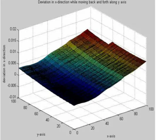
A consequent elaboration made with Matlab [47]of the obtained data has brought an interesting behaviour of the straightness (deviation in the X/Y direction moving the Y/X stage back and forth along while the other is steady) and linear error of both the axes, as shown in Fig. 7.2, Fig. 7.3 and Fig. 7.4. By analysing these graphs, it has been seen that:

• the absolute error of the X axis straightness increased together with the travel of the stage and reached a maximum value of 12µm;

• the absolute straightness error of both the axes varied with the position of the steady stage and was maximum when the latter was at the end of the travel;

• the linear error of the X axis varied along the travel and reached a maximum value of 3µm; it did not depend on the position of the Y stage;

• the linear error of the Y axis varied along the travel and reached a maximum value of 2µm; it depended on the position of the X stage and was maximum when X=0mm; Comparing these results with the specifications of the machine it has been noticed that the values found are bigger than those expected (see Paragraph 3.1). Moreover the tests were done with an external measuring system: in this way the measurement is not affected by the error due to the feedback control system and can be considered a more confident setup. Unfortunately the test was done only one time; it was not statistically enough to give a reliable results. Therefore it has been necessary to test the performances of the setup again with some designed methods to double check the values obtained. Given that the straightness error test gave the worst results, it has been decided to evaluate it and comparing the obtained values with those got from the Heidenhain test and the calibration file of the setup from Aerotech.

Furthermore some graphs (see Appendix A) were given by the builder of the machine; those represent the results of the calibration that has been made on the setup. These even disagree with the Heidenhain data.

7.2

Design of method

In order to measure the straightness of the axis it is requested to move the stage and measure the deviation from a reference point along the perpendicular direction, while keeping the other stage steady. Thus it is necessary to have a measuring instrument that is capable to detect a deviation in the order of sub-microns and to have an appropriate experimental setup.

The first idea that has been thought was to take the lateral surface of the stage as a reference directly, which is indicated in Fig. 7.5 by the white arrow. The problem in taking the lateral surface as reference would be the influence of the manufacturing errors that could be present on the stage surface. A non-flatness surface indeed would fake the measurement. Moreover there are no specifics on the surface roughness of the stage, thus even the surface finish would badly influence the measurement.

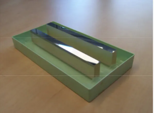
It has been chosen then to use a high precision mirror as the reference, which is positioned on the upper stage (Y stage), while the potential deviation is measured with the laser sensor Keyence LC2440.

The mirror, shown in Fig. 7.6, is on the lateral surface of a parallelepiped of 10x30x150mm. It has a surface roughness lower than 0,1µm.

Fig. 7.5- Lateral surface of the stage

7.3

Experimental setup

The mirror has been positioned on the X stage and fastened with two stirrup that have been in turn screwed to the same stage by two bolts. Two other bolts have been screwed into the stage to refer the mirror to, in order to position it as parallel as possible to the lateral surface of the stage. Given that the sensor requires a distance of 1mm from the target, the mirror has been positioned so that it has been almost in line with the lateral surface of the stage. In this way the sensor was at the right distance from the target in spite of all the obstacles due to the machine encumbrance.

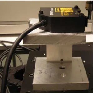
To position the sensor in the experimental setup it has been used the same clamping system (Fig. 7.7) used to hold it in the experiment for the static stiffness evaluation (see Chapter 5). This clamping system was slender enough to position the sensor close to the mirror surface.

Fig. 7.7- Sensor fixed on the camping system

The measurement of the straightness took place by moving the stage and the above fixed mirror while measuring the displacement in the orthogonal direction with the laser sensor.

The stage started from an initial position of 0mm and moved step by step until the final position of 100mm. It moved to the subsequent position and there it stopped. Then in this position the sensor recorded the value of the possible displacement that the mirror surface could have undergone during the move.

In order to obtain accurate results it has been chosen to move the stage of 5mm per each step. Therefore twenty-one values have been recorded during the move of the stage under test.

The same test has been made for each stage in different positions of the other stage that has remained steady. In order to relate the results obtained in this experiment to the Heidenhain results it has been chosen to repeat the measurements of each stage in the following positions of the other: 0mm, 20mm, 40mm, 60mm, 80mm and 100mm.

Fig. 7.8- Positions of the sensor: (white point) X straightness measurement and (red point) Y straightness measurement

The mirror position has been changed depending on which stage was under test, putting the reflective surface always parallel to the direction whose stage straightness was being measured, so as the sensor has been placed in two different positions (Fig. 7.8) to make the right measurement.

Originally in the test the sensor was reset to zero at the beginning of the stage move (0mm) and the measurements were in order recorded in relation to the previous value. Given that the sensor showed a bad stability of the values displayed in each measurement, as if the surface was too reflective to give back a stable signal, it has been decided to reset to zero the sensor every time the stage stopped. In this way the errors of each measurement have not been add up to the subsequent. Moreover it has been activated a function of the sensor that compensates the brightness of the reflective surface, so that there were less errors in the recorded value of the deviation.

This setup did not allow measuring an absolute error because:

• the mirror is positioned on the machine under test and the measure could be affected by the machine’s assembly error;

• the mirror position respect to the lateral surface is not accurate. Thus only the relative error has been measured.

7.4

Experimental result

The experiments have been conducted on both stages and the results are listed below.

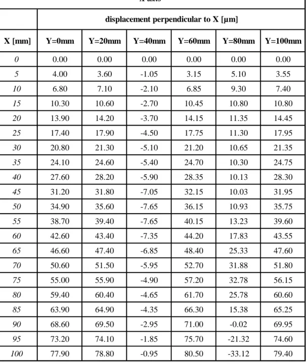
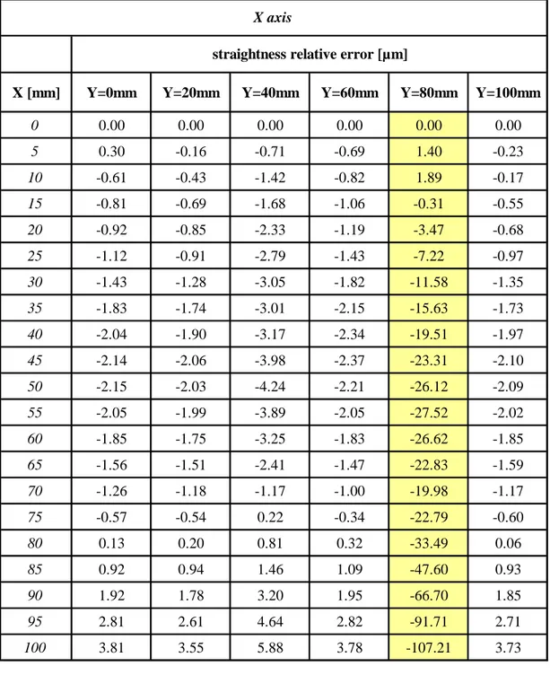
Tab. 7.1 lists the values of the deviation perpendicular to the X axis obtained moving the stage step by step along six different positions of the Y stage and recorded by the sensor. Tab. 7.2 instead shows the value of the straightness relative error of the same axis obtained as difference between the deviation measured through the experiment and the deviation of these values from the trend line proper of these data points.

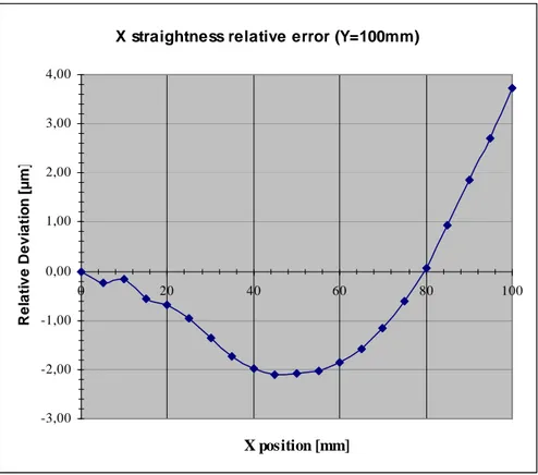
Fig. 7.9 and Fig. 7.10 display the behaviour of the X stage straightness relative error in two different positions of the Y stage: 20mm and 100mm. The graphs relative to the other positions of the Y stage are not shown because the trend of their curves is similar to those presented.

Tab. 7.3 lists the values of the deviation perpendicular to the Y axis obtained moving the stage step by step along six different positions of the X stage and recorded by the sensor. Tab. 7.4 instead shows the value of the straightness relative error obtained as difference between the deviation measured through the experiment and the deviation of these values from the trend line proper of these data points.

Fig. 7.11 and Fig. 7.12 display the behaviour of the Y stage straightness relative error in two different positions of the X stage: 0mm and 20mm. The graphs relative to the other positions of the X stage are not shown because the trend of their curves is similar to those presented.

Tab. 7.1-Perpendicular deviation (X axis)

X [mm] Y=0mm Y=20mm Y=40mm Y=60mm Y=80mm Y=100mm

0 0.00 0.00 0.00 0.00 0.00 0.00 5 4.00 3.60 -1.05 3.15 5.10 3.55 10 6.80 7.10 -2.10 6.85 9.30 7.40 15 10.30 10.60 -2.70 10.45 10.80 10.80 20 13.90 14.20 -3.70 14.15 11.35 14.45 25 17.40 17.90 -4.50 17.75 11.30 17.95 30 20.80 21.30 -5.10 21.20 10.65 21.35 35 24.10 24.60 -5.40 24.70 10.30 24.75 40 27.60 28.20 -5.90 28.35 10.13 28.30 45 31.20 31.80 -7.05 32.15 10.03 31.95 50 34.90 35.60 -7.65 36.15 10.93 35.75 55 38.70 39.40 -7.65 40.15 13.23 39.60 60 42.60 43.40 -7.35 44.20 17.83 43.55 65 46.60 47.40 -6.85 48.40 25.33 47.60 70 50.60 51.50 -5.95 52.70 31.88 51.80 75 55.00 55.90 -4.90 57.20 32.78 56.15 80 59.40 60.40 -4.65 61.70 25.78 60.60 85 63.90 64.90 -4.35 66.30 15.38 65.25 90 68.60 69.50 -2.95 71.00 -0.02 69.95 95 73.20 74.10 -1.85 75.70 -21.32 74.60 100 77.90 78.80 -0.95 80.50 -33.12 79.40 X axis displacement perpendicular to X [µm]

Tab. 7.2-Straightness relative error value (X axis)

X [mm] Y=0mm Y=20mm Y=40mm Y=60mm Y=80mm Y=100mm

0 0.00 0.00 0.00 0.00 0.00 0.00 5 0.30 -0.16 -0.71 -0.69 1.40 -0.23 10 -0.61 -0.43 -1.42 -0.82 1.89 -0.17 15 -0.81 -0.69 -1.68 -1.06 -0.31 -0.55 20 -0.92 -0.85 -2.33 -1.19 -3.47 -0.68 25 -1.12 -0.91 -2.79 -1.43 -7.22 -0.97 30 -1.43 -1.28 -3.05 -1.82 -11.58 -1.35 35 -1.83 -1.74 -3.01 -2.15 -15.63 -1.73 40 -2.04 -1.90 -3.17 -2.34 -19.51 -1.97 45 -2.14 -2.06 -3.98 -2.37 -23.31 -2.10 50 -2.15 -2.03 -4.24 -2.21 -26.12 -2.09 55 -2.05 -1.99 -3.89 -2.05 -27.52 -2.02 60 -1.85 -1.75 -3.25 -1.83 -26.62 -1.85 65 -1.56 -1.51 -2.41 -1.47 -22.83 -1.59 70 -1.26 -1.18 -1.17 -1.00 -19.98 -1.17 75 -0.57 -0.54 0.22 -0.34 -22.79 -0.60 80 0.13 0.20 0.81 0.32 -33.49 0.06 85 0.92 0.94 1.46 1.09 -47.60 0.93 90 1.92 1.78 3.20 1.95 -66.70 1.85 95 2.81 2.61 4.64 2.82 -91.71 2.71 100 3.81 3.55 5.88 3.78 -107.21 3.73 X axis

Fig. 7.9-Straightness relative error of the X axis (Y=20mm)

Fig. 7.10-Straightness relative error of the X axis (Y=100mm)

X straightness relative error (Y=20mm)

-3,00 -2,00 -1,00 0,00 1,00 2,00 3,00 4,00 0 20 40 60 80 100 X position [mm] R e la ti v e D e v ia ti o n [ µ m ]

X straightness relative error (Y=100mm)

-3,00 -2,00 -1,00 0,00 1,00 2,00 3,00 4,00 0 20 40 60 80 100 X position [mm] R e la ti v e D e v ia ti o n [ µ m ]

Tab. 7.3- Perpendicular deviation values (Y axis) Y [mm] X=0mm X=20mm X=40mm X=60mm X=80mm X=100mm 0 0,00 0,00 0,00 0,00 0,00 0,00 5 1,45 1,45 -2,35 0,50 0,95 1,05 10 2,88 2,90 -2,50 0,48 1,90 1,95 15 4,33 4,25 -2,55 0,97 2,80 2,75 20 5,75 5,62 -2,40 1,12 3,75 3,70 25 7,15 7,01 -2,10 1,67 4,75 4,65 30 8,57 8,41 -2,00 2,00 5,65 5,60 35 9,94 9,74 -1,95 2,29 6,45 6,45 40 11,27 11,12 -1,99 2,43 7,40 7,30 45 12,60 12,40 -1,84 2,73 8,30 8,25 50 13,90 13,69 -1,59 2,93 9,15 9,05 55 15,28 15,05 -1,34 3,12 10,00 9,95 60 16,58 16,32 -1,29 3,22 10,85 10,85 65 17,86 17,56 -1,19 3,37 11,75 11,70 70 19,13 18,82 -1,04 3,52 12,55 12,50 75 20,45 20,16 -0,79 3,77 13,45 13,30 80 21,61 21,34 -0,54 3,97 14,15 13,90 85 22,92 22,64 0,21 4,32 15,05 14,85 90 24,12 23,84 0,06 4,57 15,80 15,55 95 25,37 25,04 0,41 5,02 16,55 16,30 100 26,56 26,27 0,66 5,42 17,35 17,10 displacement perpendicular to Y [µm] Y axis

Tab. 7.4- Straightness relative error value (Y axis) Y X=0 X=20 X=40 X=60 X=80 X=100 0 0,00 0,00 2,50 0,00 0,00 0,00 5 0,09 0,11 0,03 0,23 0,06 0,17 10 0,16 0,22 -0,25 -0,05 0,12 0,19 15 0,25 0,23 -0,42 0,17 0,13 0,11 20 0,32 0,26 -0,40 0,05 0,19 0,18 25 0,36 0,31 -0,23 0,34 0,30 0,25 30 0,42 0,37 -0,25 0,40 0,31 0,32 35 0,43 0,36 -0,33 0,42 0,22 0,29 40 0,40 0,40 -0,49 0,30 0,28 0,26 45 0,37 0,34 -0,47 0,33 0,29 0,33 50 0,32 0,29 -0,35 0,27 0,25 0,25 55 0,34 0,31 -0,22 0,19 0,21 0,27 60 0,28 0,24 -0,30 0,02 0,17 0,29 65 0,20 0,14 -0,32 -0,09 0,18 0,26 70 0,11 0,06 -0,30 -0,21 0,09 0,18 75 0,07 0,06 -0,18 -0,23 0,10 0,10 80 -0,13 -0,10 -0,05 -0,29 -0,09 -0,18 85 -0,17 -0,14 0,57 -0,21 -0,08 -0,11 90 -0,33 -0,28 0,30 -0,23 -0,22 -0,29 95 -0,44 -0,42 0,52 -0,04 -0,36 -0,42 100 -0,61 -0,53 0,64 0,09 -0,45 -0,50 Y axis

Fig. 7.11- Straightness relative error of the Y axis (X=0mm)

Fig. 7.12- Straightness relative error of the Y axis (X=20mm)

Y straightness relative error (X=0mm)

-0,80 -0,60 -0,40 -0,20 0,00 0,20 0,40 0,60 0 20 40 60 80 100 Y position [mm] R e la ti v e D e v ia ti o n [ µ m ]

Y straightness relative error (X=20mm)

-0,80 -0,60 -0,40 -0,20 0,00 0,20 0,40 0,60 0 20 40 60 80 100 Y position [mm] R e la ti v e D e v ia ti o n [ µ m ]

7.5

Analysis and discussion

The measurements done in this experiment gave some interesting results. First it seems opportune to analyse the values obtained during the moves.

The yellow column in Tab. 7.2 has values that disagree with the others, so those results must be considered wrong. The setup perhaps failed this measurement.

As said before, the sensor has been reset to zero every move of 5mm; therefore the value read on its display was the deviation of the stage relative to the previous position. So it is not possible to talk about an absolute error, even because of the problems relative to the setup, but it may be used the behaviour of the straightness around the trend line calculated for each graph that is a sort of fluctuation around the zero value.

Analysing the graphs it is noticeable that:

• the maximum value of the relative error of the X axis is almost 4µm obtained in Y=0mm;

• the maximum value of the relative error of the Y axis is almost 0,61µm obtained in X=0mm;

• the value of the X axis relative error is one order bigger of the one of the Y axis and it is valid for each position of the steady stage.

It is not possible to make a direct comparison with the Heidenhain test results shown in Fig. 7.13 and Fig. 7.14, because these are trends of absolute error values. In order to overcome this problem the Heidenhain data have been elaborated to plot the error values relative to the trend line. To compare the results it has been calculated the deviation of the Heidenhain data point from the proper trend line, obtaining the behaviour of the straightness relative error (Fig. 7.15 and Fig. 7.16).

X Straightness error from Heidenhain data

(Y=20mm) y = 0,065x R2 = 0,6606 0 2 4 6 8 10 12 14 0 20 40 60 80 100 X position[mm] D e v ia ti o n [ µ m ]

Fig. 7.14- Absolute error Y stage (X=0mm), Heidenhain result

Fig. 7.15-X straightness relative error (Y=20mm), Heidenhain result

Y Straightness error from Heidenhain data

(X=0mm) y = 0,0275x R2 = 0,9446 0 0,5 1 1,5 2 2,5 3 3,5 0 20 40 60 80 100 Y position [mm] D e v ia ti o n [ µ m ]

X Relative error from Heidenhain: deviation from the trend line (Y=20mm)

-3 -2 -1 0 1 2 3 4 5 0 20 40 60 80 100 X position [mm] R e la ti v e e r r o r [µ m ]

Fig. 7.16- Y straightness relative error (X=0mm), Heidenhain result

Two trend lines are considered: the one from the Heidenhain test represents the axis that the stage moved along; the one from the “mirror” experiment represents indeed the axis that the stage moved along added to the error due to the position of the mirror onto the stage.

For that reason it is not possible to compare the whole behaviour of the relative error curves (Fig. 7.15 and Fig. 7.16) but only the order of magnitude of the maximum error. In Tab. 7.5 there is a summary of the maximum relative errors found in both the tests.

Tab. 7.5-Maximum relative error found in Heidenhain and “mirror” tests In conclusions it can be said that:

• the double check results showed a similarity to those obtained from the Heidenhain test although there are some different at the magnitude; therefore the Heidenhain data can be

Y Relative error from Heidenhain: deviation from the trend line (X=0mm)

-0,4 -0,3 -0,2 -0,1 0 0,1 0,2 0,3 0,4 0,5 0,6 0 20 40 60 80 100 Y position [mm] R e la ti v e e r r o r [ µ m ]

Maximumm relative error [µm]

X axis Y axis

Heidenhain test Experimental result

4.62 5.88

• the biggest error appeared at the end of travel and this can be due to both the control system, which might have problem in the response when the stages are at the extremities of the travel, and the assembly. At the first impression it can be said that the stages are not perfectly assembled, but to prove that it would be necessary to know the drawings of the machine that were not available. Having at disposal the drawings of the stages it could be taken into account the influence of the positioning encoder that read the position of the stage and send the signal to the controller. Knowing its position it could be said in which way the positioning measurement is done and how much the encoder invalidates the measurement result;

• as regard the mirror there is a problem in its position; in fact when positioning the mirror on the stage it is not possible to be sure about its precision, which is of course influenced by the stage itself. In order to have the confidence of the accurate position of the mirror a better clamping system would occur. It could be fixed to the foundation of the machine that would be as an external reference for the mirror.

• for the Heidenhain measurement, there could be an error induced by the temperature difference between the glass encoder and the environment, and by the clamping device of the glass encorder.

• during the measurement, the value on the display of the sensor was stable. It could be from the fact that the surface of the mirror is too reflective for this sensor and the signal was disturbed.