D
OCTORALT
HESISStudy and development of innovative
strategies for energy-efficient cross-layer
design of digital VLSI systems based on
Approximate Computing
Author:
Giulia STAZI
Supervisor:
Dr. Francesco MENICHELLI
A thesis submitted in fulfillment of the requirements for the degree of Doctor of Philosophy
in the
Department of Information Engineering, Electronics and Telecommunications (DIET)
Declaration of Authorship
I, Giulia STAZI, declare that this thesis titled, “Study and development of innovative strategies for energy-efficient cross-layer design of digital VLSI systems based on Approximate Computing” and the work presented in it are my own. I confirm that: • This work was done wholly or mainly while in candidature for a research
de-gree at this University.
• Where any part of this thesis has previously been submitted for a degree or any other qualification at this University or any other institution, this has been clearly stated.
• Where I have consulted the published work of others, this is always clearly attributed.
• Where I have quoted from the work of others, the source is always given. With the exception of such quotations, this thesis is entirely my own work.
• I have acknowledged all main sources of help.
• Where the thesis is based on work done by myself jointly with others, I have made clear exactly what was done by others and what I have contributed my-self.
Signed: Date:
“
gnÀji seautìn
”LA SAPIENZA UNIVERSITY OF ROME
Abstract
Faculty of Information Engineering, Informatics and Statistics (I3S) Department of Information Engineering, Electronics and Telecommunications
(DIET)
Doctor of Philosophy
Study and development of innovative strategies for energy-efficient cross-layer design of digital VLSI systems based on Approximate Computing
by Giulia STAZI
The increasing demand on requirements for high performance and energy effi-ciency in modern digital systems has led to the research of new design approaches that are able to go beyond the established energy-performance tradeoff. Looking at scientific literature, the Approximate Computing paradigm has been particularly prolific. Many applications in the domain of signal processing, multimedia, com-puter vision, machine learning are known to be particularly resilient to errors occur-ring on their input data and duoccur-ring computation, producing outputs that, although degraded, are still largely acceptable from the point of view of quality. The Ap-proximate Computing design paradigm leverages the characteristics of this group of applications to develop circuits, architectures, algorithms that, by relaxing de-sign constraints, perform their computations in an approximate or inexact manner reducing energy consumption.
This PhD research aims to explore the design of hardware/software architectures based on Approximate Computing techniques, filling the gap in literature regard-ing effective applicability and derivregard-ing a systematic methodology to characterize its benefits and tradeoffs.
The main contributions of this work are:
• the introduction of approximate memory management inside the Linux OS, allowing dynamic allocation and de-allocation of approximate memory at user level, as for normal exact memory;
• the development of an emulation environment for platforms with approximate memory units, where faults are injected during the simulation based on mod-els that reproduce the effects on memory cells of circuital and architectural techniques for approximate memories;
• the implementation and analysis of the impact of approximate memory hard-ware on real applications: the H.264 video encoder, internally modified to al-locate selected data buffers in approximate memory, and signal processing ap-plications (digital filter) using approximate memory for input/output buffers and tap registers;
• the development of a fully reconfigurable and combinatorial floating point unit, which can work with reduced precision formats.
Contents
Declaration of Authorship iii
Abstract vii
1 Introduction 1
1.1 Need for Low Power Circuit Design . . . 1
1.2 Source of Power Dissipation . . . 3
1.3 Approximate Computing . . . 5
1.4 Contribution and thesis organization . . . 7
2 Approximate Computing: State of the Art 11 2.1 Approximate Computing: main concepts . . . 11
2.2 Strategies for Approximate Computing . . . 12
2.2.1 Algorithmic and programming language Approximate Com-puting . . . 12
2.2.2 Instruction level Approximate Computing . . . 14
2.2.3 Data-level Approximate Computing . . . 14
2.2.4 ETAs - Error Tolerant Applications . . . 15
2.2.5 Approximate Computing ad hoc . . . 16
Approximate Adders. . . 16
Approximate Multipliers . . . 18
Algorithmic Noise Tolerance and Reduced Precision Redun-dancy techniques . . . 20
2.2.6 Design automation Approximate Computing or functional ap-proximation. . . 21
ABACUS . . . 22
2.2.7 Approximate Computing metrics. . . 23
Performance metrics . . . 23
Quality metrics . . . 23
2.3 Approximate Memories . . . 25
2.3.1 Approximate Memory Circuits and Architectures . . . 25
Approximate SRAM . . . 25
Approximate DRAM . . . 27
2.4 Transprecision Computing . . . 32
2.5 Approximate Computing and Machine Learning . . . 33
3 Approximate Memory Support in Linux OS 39 3.1 Introduction . . . 39
3.2 Linux Memory Management . . . 40
3.2.1 Virtual Memory and Address Spaces. . . 40
3.2.2 Low Memory and High Memory . . . 41
3.2.3 Physical Memory . . . 42
Page-level allocator (Buddy System algorithm) . . . 46
Continuous Memory Allocator Kmalloc . . . 48
Non Contiguous Memory Allocator vmalloc . . . 49
3.3 Development of approximate memory management in Linux Kernel . 50 3.3.1 Kernel compile-time configuration menu . . . 50
3.3.2 Creation of ZONE_APPROXIMATE on 32-bit architectures. . 51
ZONE_APPROXIMATE on x86 architectures . . . 53
ZONE_APPROXIMATE on ARM architectures. . . 56
ZONE_APPROXIMATE on RISC-V 32-bit architectures . . . . 60
3.3.3 Approximate Memory and Early Boot Allocators . . . 61
3.4 Allocation in ZONE_APPROXIMATE . . . 64
3.4.1 Approximate GFP Flags . . . 64
Alloc Fair policy . . . 66
3.4.2 User level approximate memory allocation . . . 67
3.4.3 Implementation of the device /dev/approxmem. . . 68
3.4.4 Approximate Memory Library: approx_malloc and approx_free 73 approx_malloc . . . 73
approx_free . . . 74
3.4.5 Initial verification . . . 75
3.5 Quality Aware Approximate Memory Zones in Linux OS . . . 78
3.5.1 Introduction and 64-bit implementation potentials. . . 78
3.5.2 Approximate memory zones on 64-bit architectures . . . 79
3.5.3 Data Allocation . . . 81
approx library for multiple approximate memory zone . . . 82
3.5.4 Initial verification of the implementation . . . 83
3.5.5 Verification and allocation tests . . . 83
4 AppropinQuo, Full System Emulator for Approximate Memory Platforms 89 4.1 Introduction . . . 89
4.2 Related Works: Simulation environments for digital platforms . . . 90
4.3 QEmu Emulator . . . 91
4.3.1 Main Concepts . . . 91
4.3.2 Dynamic Translation: Tiny Code Generator . . . 92
4.3.3 QEmu SoftMMU . . . 92
4.4 Approximate Memory in ApropinQuo . . . 93
4.4.1 QEmu Memory Management . . . 93
Approximate memory mapping on PC PIIX, x86 architecture . 94 Approximate memory mapping on Vexpress Cortex A9, ARM architecture . . . 95
Approximate memory mapping on VirtIO, RISCV-32 architec-ture . . . 97
Multiple Approximate memories mapping on VirtIO, RISC-V64 architecture . . . 97
4.4.2 Approxmem device in AppropinQuo . . . 98
4.5 Error injection models for approximate memories . . . 101
4.5.1 DRAM orientation dependent models . . . 101
4.5.2 SRAM models . . . 104
Error on read . . . 104
Error on write . . . 105
4.5.3 Bit dropping fault model . . . 105
4.6 Quality aware selective ECC for approximate DRAM and model. . . . 107
4.6.1 Bit dropping for LSBs, bit reuse and selective ECC . . . 108
4.6.2 Quality aware selective ECC . . . 108
ECC codes for approximate memories . . . 108
4.6.3 Impact of bit dropping and bit reuse . . . 109
4.6.4 Implementation . . . 109
4.7 Verification of fault models . . . 111
4.7.1 Error on access models verification . . . 111
4.7.2 DRAM orientation model verification . . . 111
4.7.3 Bit dropping model verification. . . 112
5 Exploiting approximate memory in applications and results 115 5.1 Introduction . . . 115
5.2 Impact of Approximate Memory on a H.264 Software Video Encoder . 116 5.2.1 H.264 video encoding and the x264 encoder . . . 116
H.264 Encoder . . . 117
H.264 Decoder . . . 118
H.264 data fault resilience . . . 118
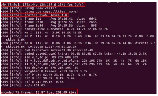
The x264 software video encoder . . . 118
Analysis of x264 heap memory usage . . . 119
5.2.2 Approximate memory data allocation for the x264 encoder . . . 120
5.2.3 Experimental setup . . . 123
5.2.4 Impact on output using approximate DRAM and power sav-ing considerations . . . 124
Power saving considerations . . . 126
5.2.5 Impact on output using approximate SRAM . . . 127
5.2.6 Considerations on the results and possible future analysis . . . 128
5.3 Study of the impact of approximate memory on a digital FIR filter design. . . 129
Impact on output using approximate DRAM . . . 131
Impact on output using approximate SRAM . . . 132
Impact on output using approximate SRAM with bit dropping 132 5.4 Quality aware approximate memories, an example application on dig-ital FIR filtering . . . 133
6 Synthesis Time Reconfigurable Floating Point Unit for Transprecision Com-puting 137 6.1 Introduction and previous works . . . 137
6.2 Floating Point representation, IEEE-754 standard . . . 138
6.3 Design of the reconfigurable Floating Point Unit . . . 139
6.3.1 Top unit Floating_Point_Unit_core . . . 140
6.4 Experimental Results . . . 144
6.4.1 Testing . . . 144
6.4.2 Synthesis Setup . . . 144
6.4.3 Results . . . 145
Number of gates and resources . . . 145
Propagation delay and speed . . . 146
Power consumption . . . 147
7 Conclusion 149
7.1 Approximate Memory management within the Linux Kernel . . . 149
7.2 Models and emulator for microprocessor platforms with approximate memory . . . 151
7.3 Impact of approximate memory allocation on ETAs . . . 152
7.4 Transprecision FPU implementation . . . 153 A Linux kernel files for approximate memory support 155
A.1 Patched Kernel files . . . 155
A.2 New Kernel source files . . . 156
A.3 Approximate Memory Configuration (Make menuconfig). . . 156 B AppropinQuo: list of approximate memory models 157
B.0.1 QEmu 2.5.1 patched files for approximate memory support . . 157
B.0.2 New QEmu 2.5.1 source files . . . 157
C Transprecision FPU: list of vhd files 159
D Publications and Presentations 161
List of Figures
1.1 Dennard scaling and power consumption models. Source: Hennessy,
2018 . . . 1
1.2 Moore’s law. Source: . . . 2
1.3 Amdahl’s law. Source: . . . 3
1.4 Dark silicon:end of multicore era. Source: Hardavellas et al.,2011 . . . 4
1.5 Power trends. Source: [Burns,2016] . . . 5
1.6 Power trends. Source: [Energy Aware Scheduling] . . . 6
1.7 Low power strategies at different abstraction levels. Source: [Gupta and Padave,2016] . . . 7
2.1 Overview of ASAC framework. Source: Roy et al.,2014 . . . 12
2.2 Overview of ARC framework. Source: Chippa et al.,2013 . . . 13
2.3 Overview of EnerJ language extension. Source: Sampson et al.,2011 . 14
2.4 ISA extension for AxC support. Source: Esmaeilzadeh et al.,2012 . . . 15
2.5 Examples of ETAs . . . 15
2.6 Possible sources of application error resilience .Source: Chippa et al.,
2013 . . . 16
2.7 a) simplified MA, b) approximation 1, c) approximation 2. Source:Gupta et al.,2011 . . . 17
2.8 Design of exact full adder, 10 transistors. Source: Yang et al.,2013 . . . 17
2.9 Design of AXA1, 8 transistors. Source: Yang et al.,2013 . . . 18
2.10 Design of AXA2, 6 transistors. Source: Yang et al.,2013 . . . 18
2.11 Design of AXA3, 8 transistors .Source: Yang et al.,2013 . . . 18
2.12 Comparison between AXA1, AXA2, AXA3 and exact full adder .Source: Yang et al.,2013 . . . 19
2.13 Overview of approximate multipliers comparison. Source: Masadeh, Hasan, and Tahar,2018 . . . 19
2.14 Overview of different approximate FA properties. Source: Masadeh, Hasan, and Tahar,2018 . . . 20
2.15 Reduced Precision Redundancy ANT Block Diagram. Source: Pagliari et al.,2015 . . . 21
2.16 Determining the Hamming distance of two combinational circuits us-ing a Binary Decision Diagrams (BDD). Source : Vasicek and Sekan-ina,2016 . . . 22
2.17 Integration of ABACUS in a traditional design flow. Source : Nepal et al.,2014 . . . 23
2.18 SRAM bit dropping precharge circuit. Source: Frustaci et al.,2016 . . . 27
2.19 Sram SNBB precharge circuit. Source: Frustaci et al.,2016 . . . 27
2.20 Architecture of dual Vddmemory array. Source : Cho et al.,2011 . . . . 28
2.21 Overview of HW/SW components for approximated caches. Source : Shoushtari, BanaiyanMofrad, and Dutt,2015 . . . 28
2.23 Proposed DRAM partitioning according to refresh rate. Source : Liu
et al.,2012b. . . 29
2.24 Proposed mapping of bits of 4 DRAM chips. Source : Lucas et al.,2014 30 2.25 Proposed quality bins. Source : Raha et al.,2017 . . . 30
2.26 eDRAM emulator: block diagram. Source: Widmer, Bonetti, and Burg, 2019 . . . 31
2.27 Benchmarks output quality for refuced refresh rate. Source: Widmer, Bonetti, and Burg,2019 . . . 32
2.28 Transprecision Computing paradigm. Source : Malossi et al.,2018 . . . 32
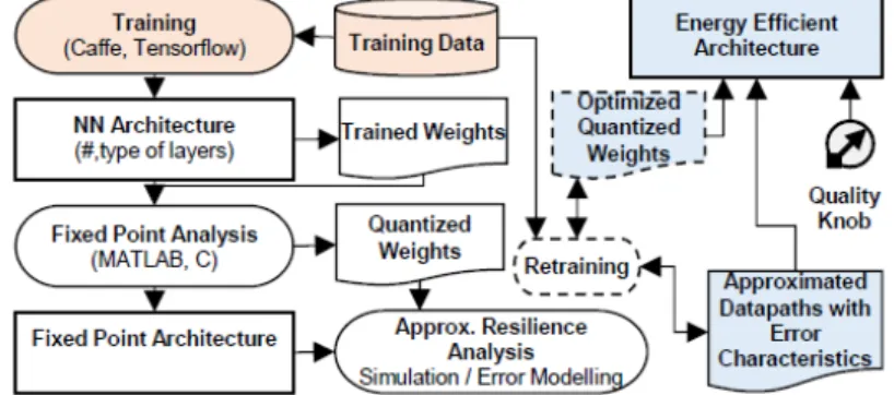
2.29 Methodology for designing energy-effcient and adaptive neural net-work accelerator-based architectures for Machine Learning. Source: Shafique et al.,2017a . . . 33
2.30 Overview of DRE. Source : Chen et al.,2017 . . . 35
2.31 Flow of Single Layer Analysis. Source: Chen et al.,2017 . . . 35
2.32 Approximate memory architecture; (a) conventional data storage scheme, (b) approximate data storage scheme, (c) system architecture to sup-port approximate memory access. Source: Nguyen et al.,2018 . . . 36
2.33 Row-level refresh scheme for approximate DRAM. Source: Nguyen et al.,2018 . . . 37
3.1 Kernel address space and User process address space . . . 42
3.2 Nodes, Zones and Pages. Source:[Gorman,2004] . . . 42
3.3 Zone watermarks . . . 44
3.4 Buddy system allocator. . . 46
3.5 The linear address interval starting from PAGE_OFFSET. Source: [Bovet, 2005] . . . 50
3.6 Example of menuconfig menu for x86 architecture . . . 51
3.7 Output of dmesg command. . . 57
3.8 Output of cat /proc/zoneinfo command . . . 57
3.9 Device tree structure . . . 58
3.10 Example of approximate memory node in DTB file . . . 59
3.11 Vexpress Cortex A9 board memory map (extract). . . 60
3.12 On left: kernel boot logs. On right: zone_approximate statistics . . . . 60
3.13 RISC-V Boot messages . . . 61
3.14 Overview of memory allocators. Source:[Liu,2010] . . . 62
3.15 Memblock memory allocation . . . 63
3.16 Memblock allocator function tree . . . 63
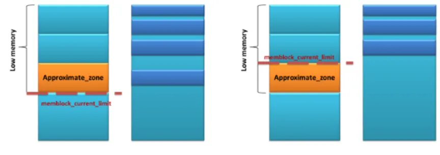
3.17 Memblock current limit on architectures with ZONE_APPROXIMATE 64 3.18 Output of cat /proc/zoneinfo command . . . 64
3.19 Device driver interaction . . . 68
3.20 Creation of device approxmem . . . 73
3.21 Bulding the linked list . . . 76
3.22 vmallocinfo messages on x86 architecture . . . 76
3.23 Messages of cat / proc / pid / maps . . . 77
3.24 ZONE_APPROXIMATEstatistics after boot . . . 77
3.25 ZONE_APPROXIMATEstatistics after approx_malloc call . . . 77
3.26 Configuration of physical memory layout . . . 81
3.27 Configuration of physical memory layout on RISC-V SiFiveU . . . 83
3.28 Boot messages printing the physical memory layout . . . 84
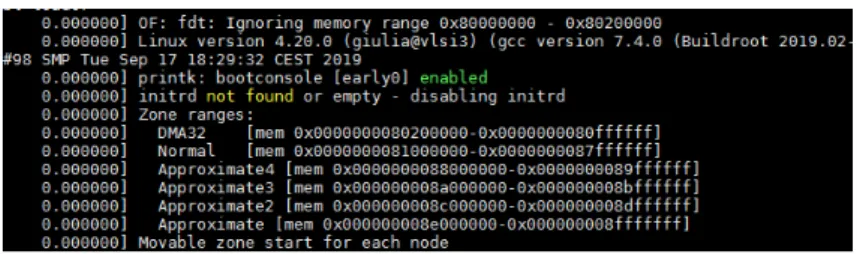
3.29 Kernel boot messages for RISCV 64 platform with 4 approximate mem-ory zones . . . 84
3.30 ZONE_APPROXIMATEstatistics after approx_malloc call . . . 86
3.31 ZONE_APPROXIMATE2 statistics after approx_malloc call . . . 87
3.32 ZONE_APPROXIMATE3 statistics after approx_malloc call . . . 87
3.33 ZONE_APPROXIMATE4 statistics after approx_malloc call . . . 87
4.1 Tiny Code Generator . . . 92
4.2 QEmu SoftMMU . . . 93
4.3 e820 Bios Memory Mapping passed to Linux Kernel . . . 96
4.4 DRAM true cell and anti cell. Source:Liu et al.,2013 . . . 102
4.5 Error on Read debug messages produced during execution . . . 105
4.6 SRAM precharge circuit for bit-dropping technique. Source:Frustaci et al.,2015a . . . 106
4.7 Example of Looseness Mask on Big Endian architecture . . . 107
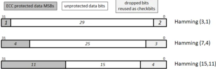
4.8 32 bit ECC data format in approximate memory . . . 110
5.1 H.264 high level coding/decoding scheme . . . 117
5.2 H.264 inter-frame and intra-frame prediction . . . 117
5.3 x264 encoding information. . . 119
5.4 Memory allocation profiling: Massif output . . . 120
5.5 x264, output frame with different Looseness Levels and fault rate 10−4 [errors/(bit×s)] . . . 125
5.6 x264, output frame with different Looseness Levels and fault rate 10−3 [errors/(bit×s)] . . . 125
5.7 Video Output PSNR graph [dB] . . . 127
5.8 DRAM cell retention time distribution. Source:Liu et al.,2012a . . . 127
5.9 x264, output frame coded with exact (top left) and approximate SRAM (0xFFFFFFFF looseness mask), fault rate 10−6(top right), 10−4(bottom left) and 10−2(bottom right) [errors/access].. . . 129
5.10 Digital FIR architecture . . . 130
5.11 FIR, output SNR [dB] for approximate DRAM (anti cells) . . . 132
6.1 Block diagram of the FPU hardware datapath. Source:[Tagliavini et al.,2018] . . . 138
6.2 IEEE 754 Precision formats. . . 139
6.3 Floating Point Unit Core architecture . . . 141
6.4 External interface of FPU core . . . 142
6.5 Resources with DSP disabled @40MHz. . . 145
6.6 Resources with DSP disabled @40MHz: from half to double precision . 146
List of Tables
3.1 DMA zone, physical ranges . . . 43
3.2 32-bit x86 architecture memory layout . . . 53
3.3 32-bit x86 memory layout with ZONE_APPROXIMATE . . . 54
4.1 List of Hamming codes . . . 109
4.2 FIR, output SNR [dB] . . . 109
4.3 BER for 32 bit data in approximate memory . . . 110
4.4 bench_access results, fixed Looseness Level . . . 112
4.5 bench_spontaneous_error results (Wait time t=1000ms) . . . 113
4.6 bench_dropping results. . . 113
5.1 Heap memory usage . . . 119
5.2 Test videos from derf’s collection . . . 123
5.3 Video Output PSNR [dB] . . . 126
5.4 x264, video output PSNR [dB] for approximate DRAM (true cells) . . . 126
5.5 x264, video output PSNR [dB] for approximate SRAM (error on access) 128 5.6 FIR, output SNR [dB] for SRAM. . . 133
5.7 FIR, SNR [dB] for SRAM bit dropping . . . 133
5.8 FIR, access count on approximate data structures. . . 135
5.9 FIR, output SNR [dB] for SRAM, EOR . . . 135
5.10 FIR, output SNR [dB] for SRAM, EOW . . . 135
6.1 Operation codes . . . 142
6.2 List of analyzed formats . . . 144
6.3 Resources @ 40MHz clock with DSP disabled . . . 145
6.4 Propagation delay for reduced precision FP formats . . . 146
List of Abbreviations
AxC Approximate Computing
AxM Approximate Memory
ANT Algorithmic Noise Tolerance
BDD Binary Decision Diagram
BER Bit Error Rate
CNN Convolutional Neural Network
CPS Cyber Physical System
CS Chip Select
DCT Discret Cosin Transform
DMA Direct Memory Access
DNN Deep Neural Network
DPM Dynamic Power Managment
DRAM Dynamic Random Acess Memory
DRT Data Retention Time
eDRAM embedded Dynamic Random Acess Memory
ECC Error Correction Code
EOR Error On Read
EOW Error On Write
ER Error Rate
ES Error Significance
EAS Energy Aware Scheduler
ETA Error Tolerant Application
FA Full Adder
FIR Finite Impulse Response
GFP Get Free Page
HPC High Performance Computing
HW HardWare
IoE Internet of Everything
IoT Internet of Things
ISA Instruction Set Architecture
LSB Least Significant Bit
MA Mirror Adder
ML Machine Learning
MMU Memory Management Unit
MSB Most Significant Bit
MSE Mean Squared Error
NBB Negative Bitline Boosting
OS Operating System
PDP Power Delay Product
PSNR Peak Signal to Noise Ratio
PULP Processor Ultra Low Power
QoS Quality of Service
RTL Register Transfer Level
RPR Reduced Precision Format
SoC System on Chip
SSIM Structural SIMilarity
SNBB Selective Negative Bitline Boosting
SNR Signal to Noise Ratio
SRAM Static Random Acess Memory
SW SoftWare
TCG Tiny Code Generator
TS Training Set
VLSI Very Large Scale Integration
VGG Visual Geometry Group
To my dearest affections, for always being by my side.
To myself for the constancy and commitment to achieve this
Chapter 1
Introduction
1.1
Need for Low Power Circuit Design
In the past, during the so-called desktop PC era, the main goal of VLSI design was to develop systems capable of satisfying and optimizing real time processing re-quirements, computational speed and graphics quality in applications such as video compression, games and graphics. With the advancement of VLSI technology, digi-tal systems have increased in complexity and three factors have come to convergence making energy efficiency the most important constraint:
• Technology. From a technological point of view, excessive energy consumption has become the limiting factor in integrating multiple transistors on a single chip or a multi-chip module, determining the end of the Dennard scaling law (Fig. 1.4).
FIGURE 1.1: Dennard scaling and power consumption models. Source: Hennessy,2018
The latter, also known as MOSFET scaling (1977), claims that as the transis-tors shrink in size, the power density stays constant; meaning indeed that the power consumption is proportional to the chip area. This law allowed chip-makers to increase clock speed of processors over years without increasing power. However, the MOSFET scaling, which held from 1977 to 1997, became fading between 1997 to 2006 until it collapsed rapidly in 2007 when the tran-sistors became so small that the increased leakage started overheating the chip and preventing processors from clocking up further.
In these years there has been also a slowdown in Moore’s law (Fig.1.2), accord-ing to which the number of devices in a chip doubles every 18 months [Platt,
2018]. In facts, with the end of Dennard’s law process technology scaling can continue to allow the duplication of the number of transistor for every gener-ation, but without getting a significant improvement in switching speed and energy efficiency of transistors. As the number of transistors increased, also energy consumption raising followed. Technology scaling, while involving a reduction of supply voltage (0.7 scaling factor) and a reduction in the die area (0.5 scaling factor), started increasing parasitic capacities of about 43%, mean-ing that the power density increases by 40% with each generation [Low Power Design in VLSI].
FIGURE1.2: Moore’s law. Source:
• Architecture. The limitations and inefficiencies in exploiting instruction level parallelism (dominant approach from 1982 to 2005) has led to the end of single-processor era. Moreover the Amdahl’s Law (Fig. 1.3), which aims to predict the theoretical maximum speedup for programs using multiple processors, and its implications ended the ’easy’ multicore era. Citing this law: “the effort ex-pended on achieving high parallel processing rates is wasted unless it is accompa-nied by achievements in sequential processing rates of very nearly the same magni-tude”[Amdahl,1967]. In [Esmaeilzadeh et al.,2013] it is also shown that, as the number of cores increases, constraints on power consumption can prevent all the cores from being powered at maximum speed, determining a fraction of cores which are always powered off (dark silicon). At 22 nm the 21% of a fixed-size chip must be "dark", and, with ITRS projections, at 8 nm, this number can grow up to more than 50%.
• Application focus shift. The transition from desktop PC to individual, mobile devices and ultrascale cloud computing determines the definition of new con-straints. The advent of the Big Data era, IoT technologies, IoE and CPS have led to increasing demand for data processing, storage and transmission: modern digital systems are required to interact continuously with the external physical world, satisfying not only requirements on high performance capabilities but also specific constraints on energy and power consumption.
FIGURE1.3: Amdahl’s law. Source:
Power consumption therefore has become an essential constraint in portable devices, in order to take advantage of real time execution times having min-imum possible requirements on weight, battery life and physical dimensions due to battery size. As an example, we can consider that almost 70% of users look for longer talk times and battery lasting times as a key feature for mobile phones [Natarajan et al., 2018]. Moreover, power consumption impacts sig-nificantly the design of VLSI circuits since users of mobile devices continue to demand:
– mobility: Nowadays consumers continue to request smaller and sleeker mobile devices. To support these features, high level silicon integration processes are required, which, in turn, determines high levels of leakage. Hence the need to find a strategy to reduce powr cinsumption and in particular leakage currents.
– portability: battery life is impacted by energy consumed per task; more-over a second order effect is that effective battery energy capacity is de-creased by higher drawing current that causes IR drops in power supply voltage. To overcome this issue, more power/ground pins are required to reduce the resistance R and also thicker/wider on-chip metal wires or dedicated metal layers are necessary.
– reliability. Power dissipated as heat reduces speed and reliability since high power systems tend to run hot and the temperature can exacerbate several silicon failure mechanisms. More expensive packaging and cool-ing systems are indeed required.
1.2
Source of Power Dissipation
The sources of power dissipation in a CMOS device are expressed by the elements of the following equation:
FIGURE1.4: Dark silicon:end of multicore era. Source: Hardavellas et al.,2011
TotalPowerP= Pdynamic+Pshort−circuit+Pleakage+Pstatic In particular:
• Dynamic power or switching power:
P=αCV2f
where P corresponds to the power, C is the effective switch capacitance which is a function of gate fan-out, wire length and transistor size, V is the supply voltage, f is the frequency of operation and α the switching activity factor. It corresponds to the power dissipated by charging/discharging the parasitic capacitors of each circuit node.
• Pshort−circuit:
P= IshortV
which is produced by the direct path between supply rails during switching. In particular both pull-down (n-MOS) and pull-up (p-MOS) networks may be momentarily ON simultaneously leading to an impulse of short-circuit cur-rent.
• Pleakage:
P= IleakageV
which is mainly determined by the fabrication technology. There are many sources that contribute to the leakage power, such as gate leakage, junction leakage, sub-threshold conduction. It occurs even when the system is idle or in standby mode. The leakage power, which is the dominant component in static energy consumption, was mainly neglected until 2005 when, in corre-spondence with the 65nm technology step, further scaling of threshold voltage
has extremely increased the sub-threshold leakage currents (Fig. 1.5). It is ex-pected that this kind of power will increase 32 times per device by 2020 [Roy and Prasad,2009].
• Pstatic:
P= IstaticV
which is determined by the constant current from Vdd the ground (standby power).
FIGURE1.5: Power trends. Source: [Burns,2016]
1.3
Approximate Computing
The problems caused by the sharp increase in power densities of SoC, due to the interruption of Dennard’s downsizing law, prompted the search for new solutions. There are different strategies that can be applied for reducing power consumption at different levels of the VLSI design flow [Gupta and Padave,2016, R.,2016] (Fig.1.7). These are listed below:
• Operating System and Software Level: approaches such as partitioning and com-pression algorithms. At Operating System level, power consumption can be reduced by designing an "‘energy-aware"’ scheduler (EAS). In this scenario, the scheduler takes decision relying on energy models of the resources. As an ex-ample in Linux kernel 5.4.0 the EAS, based on energy models of the CPU, is able to select an energy efficient CPU for each task [Energy Aware Scheduling] (Fig. 1.6).
OS can also achieve energy efficiency by implementing Dynamic Power Manage-ment (DPM) of system resources allowing to reconfigure dynamically the sys-tem providing the requested services [Low Power Principles]. Another approach at system level can be code compression, which proposes basically to store pro-grams in a compressed form and decompress them on-the-fly at execution time [Varadharajan and Nallasamy,2017, Benini, Menichelli, and Olivieri,2004]. An example of a simple code compression approach consists in the definition of a dense instruction set, characterized by a limited number of short instructions. This technique has been adopted by several commercial core processors such as ARM (Thumb ISA), MIPS and Xtensa.
FIGURE1.6: Power trends. Source: [Energy Aware Scheduling]
• Architecture level: techniques such as parallelism, pipelining, distributed pro-cessing and power management. In particular, parallelism and pipelining can optimize power consumption at the expense of area while maintaining the same throughput. By combining these two approaches it is possible to achieve a further reduction in power by aggressively reducing supply voltage.
• Circuit/Logic level: examples are voltage scaling, double edge triggering and transistor sizing. The latter in particular has a strong impact on circuit delay and power dissipation in combinational circuits. At logic level an example is represented by adiabatic circuits which use reversible logic to conserve energy. The implementation of these circuits is governed by two rules:
1. a transistor must never be turned on when there is a potential voltage between drain and source;
2. a transistor must never be turned off when current is flowing through it. • Technology Level: techniques such as threshold reduction and multi-threshold
(MT-CMOS) devices. The latter refers to the possibility of realizing transistors with different thresholds in a CMOS process, which allows to save energy up to 30% [Gupta and Padave,2016]. Another technique is the usage of multiple supply voltages (Voltage Islands) that, by assigning different Vddvalues to cells according to their timing criticality, allows to reduce both leakage and dynamic power. In particular, the basic idea is to group different supply voltages in a reduced number of voltage islands (each one with a single Vdd) avoiding complex power supply system and a large amount of level shifters.
In the past, across all low power approaches described above, computing plat-forms have always been designed following the principle of deterministic accuracy, for which every computational operation must be implemented deterministically and with full precision (exact computation). However, continuing to include deter-ministic accuracy in computation at all stages seems to be outperforming and dos not allow to solve the upcoming energy efficiency challenges; this stimulated the exploration of new directions in the design of modern digital systems.
Approximate Computing (AxC) is an emerging paradigm which proposes to re-duce power consumption by relaxing the specifications on fully precise or com-pletely deterministic operations. This is due to the fact that many applications, known as ETA (Error Tolerant Applications), are intrinsically resilient to errors and can produce outputs with a slightly shift in accuracy and a significant reduction in
FIGURE 1.7: Low power strategies at different abstraction levels. Source: [Gupta and Padave,2016]
computations. AxC therefore exploits the gap between the effective quality level required by applications and the one provided by the computer system in order to save energy.
Although it is an extremely promising approach, Approximate Computing is not a panacea. It is right to underline the need to accurately select where to apply AxC techniques in code and data portions. Suffice it to consider that a uncontrolled use of approximate circuits can lead to intolerable quality losses or applying approximate techniques in program control flow can lead to catastrophic events such as process or systems crashes. Finally, it is necessary to evaluate the impact of the approimate computation on output quality, in order to assess that the quality specifications are still met.
1.4
Contribution and thesis organization
The aim of this work is mainly to explore design and programming techniques for low-power microprocessor architectures based on Approximate Computing. Chap-ter2illustrates the promises and challenges of AxC, focusing on the key concepts (Section2.1), on the motivations that led to the development of this paradigm and on quality metrics. Then it is presented a survey of Approximate Computing tech-niques, from programming languages (how to automatically find approximable code/-data and support of programming languages for approximate computing, Section
2.2.1), approximate ISA (Section 2.2.2), design automation methods developed for the approximation of a class of problems (Functional Approximate Computing, Section
2.2.6), design of approximate devices and components (Approximate Computing ad hoc: approximate memories, approximate adders, approximate multipliers. Section
2.2.5). The key concepts of AxC are then compared to those of another emerging paradigm: the Transprecision Computation, born in the context of OPRECOMP, a 4-year research project funded under the EU Horizon 2020 framework. Finally, the adoption of approximate computing strategies for machine learning algorithms and architecture is illustrated.
Particular emphasis in this work has been placed on approximate memories (SRAM, DRAM, eDRAM), considering that it is expected that the power consump-tion of memories will constitute more than 50% of the entire system power. The scope of designing an architecture with approximate memories is to reduce power consumption for storing part of the data, by managing critical data and non-critical (approximate) data separately; with this partitioning it is possible to save energy
by relaxing design constraints and allowing errors on non-critical data. One of the final goals of this thesis is to provide the required tools to evaluate the impact of different levels of approximation on the target application, considering that quality output is not only impacted by the fault rate but it also depends on the application, its implementation and its representation of the data in memory.
The work starts from the software layer, implementing the support for Approxi-mate Memories (AxM) in Linux Kernel (version 4.3 and 4.20) and allowing the OS to distinguish between exact memory and approximate memory. In particular Chapter
3provides a description of the physical memory management in Linux OS kernel (Section3.2.3); then the development of the extension to support approximate mem-ory allocation is described (Section3.3). This extension has been implemented and tested for three different of architectures:
• Intel x86, as a target in the group of High Performance Computing; • ARM, as a target in the group of Embedded Systems architectures;
• RISC-V, as the emerging instruction set which is rising interest in the research and industrial communities.
In order to complete this step, it has been also necessary to implement a user-space library to allow applications to easily allocate run-time critical and non critical data in different memory areas. Finally, results are illustrated, in the form of allocation statistic messages provided by the kernel, discussing the characteristics of the im-plementation.
The next step of the work is represented by the development of AppropinQuo, a hardware emulator to reproduce the behavior of a system platforms with approxi-mate memory. This part is illustrated in Chapter4, the core of this work has been the implementation of models of the effects of approximate memory circuits and ar-chitectures, that depend on the internal structure and organization of the cells. The ability to emulate a complete platform, including CPU, peripherals and hardware-software interactions, is particularly important since it allows to execute the appli-cation as on the real board, reproducing the effects of errors on output. In fact, output quality is related not only to error rate but it also depends on the application, implementation and its data representation. The level of approximation instead is determined by key parameters such as the error rate and the number of bits that can be affected by errors (looseness level).
After the implementation of AxM support at OS level and of the emulator Ap-propinQuo, Chapter 5 describes the analysis and the implementation of different error tolerant applications modified for allocating non critical data structures in ap-proximate memory. For these applications the impact of different levels of approx-imation on the output quality has been studied. The first application is a h264 en-coder (Section 5.2). This work started by profiling memory usage and finding a strategy for selecting error tolerant data buffers. Then the modified application was run on the AppropinQuo emulator, for several combination of fault rates and fault masking at bit level (looseness level). The obtained results, showing the importance of exploring the relation between these parameters and output quality, are then ana-lyzed. The second application is a digital filter (Section5.3). In particular a 100-taps FIR filter program (configured as low-pass filter), working on audio signal, is im-plemented. The latter has been implemented to allocate tolerant data (internal tap registers and input and output buffers) on approximate memory while the FIR coef-ficients are kept exact. Results are provided in terms of SNR.
Eventually, Chapter 6, in the context of Transprecision Computing, describes the implementation of a fully combinational and reconfigurable Floating Point Unit, which can perform arithmetic operations on FP numbers with arbitrary length and structure (mantissa and exponent) up to 64 bits, included all formats defined by the IEEE-754 standard. In particular, the analysis of the resutls has been focused on re-duced precisions formats, between 16 bit (IEEE half-precision) and 32 bit (IEEE single-precision), evaluating the impact on performance, reuired area, power consumption and propagation speed.
Chapter 2
Approximate Computing: State of
the Art
2.1
Approximate Computing: main concepts
Energy savings has become a first-class constrain in the design of digital systems. Currently most of the digital computations are performed on mobile devices such as smart-phones or on large data centers (for example cloud computing systems), which are both sensitive to the topic of energy consumption. Concerning only the US data centers it is expected that the electricity consumption will increase from 61 millions kW in 2006 to 140 kW in 2020. In the era of nano-scaling, the conflict be-tween increasing performance demands and energy savings represents a significant design challenge.
In this context Approximate Computing [Han and Orshansky,2013] has become a viable approach to energy efficient design of modern digital systems.
Such an approach relies on the fact that many applications, known as Error Tol-erant Applications (see section2.2.4), can tolerate a certain degree of approximation in the output data without affecting the quality of results perceived by the user. The solutions offered by this paradigm are also supported by technology scaling fac-tors, due to the growing statistical variability in process parameters which makes traditional design methodologies inefficient [Mastrandrea, Menichelli, and Olivieri,
2011].
Approximate Computing can be implemented through different paradigms as: 1. Algorithmic level and Programming level Approximate Computing [Palem, 2003],
subsection:2.2.1;
2. Instruction level Approximate Computing [Gupta et al., 2013; Venkataramani et al.,2012; Esmaeilzadeh et al.,2012], subsection:2.2.2;
3. Data-level Approximate Computing [Frustaci et al.,2015b; Frustaci et al., 2016], section:2.2.3;
In literature several approximation methodologies are described even if two sce-narios are dominating: approximate computing ad hoc and design automation (or functional) approximate computing. These approaches will be discussed in the fol-lowing sections (2.2.5and2.2.6).
2.2
Strategies for Approximate Computing
2.2.1 Algorithmic and programming language Approximate Computing
Discovering data and operations that can be approximated is a crucial issue in ev-ery AC technique: in several cases it can turn out to be intuitive, as for example lower-order bits of signal processing applications but in other more complex cases it can require a deep dive analysis of application characteristics. Several works and techniques have been implemented in order to address this problem. In [Roy et al.,2014] the authors propose ASAC (Automatic Sensitivity Analysis for Approximate Computing), a framework which uses statistical methods to find relaxable data of ap-plications in an automatic manner. The proposed approach, as shown in Fig. 2.1, consists in the following steps:
• collect application variables and the range of values that these ones can as-sume;
• use binary instrumentation to perturb variables and compute the new output; • compare the new output to the exact one in order to measure the contribution
of each variable;
• mark a variable as approximable or not according to the results of the previous step.
FIGURE2.1: Overview of ASAC framework. Source: Roy et al.,2014
The benefits of this approach is that the programmer is not involved in the pro-cess of annotating relaxable program portions. However, a drawback is that a vari-able can be marked as approximvari-able even if it is not, leading to errors.
In [Chippa et al., 2013] the ARC (Application Resilience Characterization) frame-work is described (Fig.2.2). In this work, the authors firstly identify the application parts that could be potentially resilient, and so that could be approximated, and the sensitive parts; then they use approximation models, abstracting several AxC techniques, to characterize the resilient parts. In particular the proposed framework consists in the following steps:
• resilience identification step: identification of atomic kernels as innermost loop in which the application spends more than the 1% of its execution time. Random errors are injected in the kernel output variables, using Valgrind DBI tool. The
kernel is considered sensitive if the output does not match quality constraints, otherwise it could be resilient.
• resilience characterization step: errors are injected in the kernel using Valgrind in order to quantify the kernel resilience. In particular, using specific models such as loop perforation, inexact arithmetic circuits and so on, a quality profile of the application is produced.
FIGURE 2.2: Overview of ARC framework. Source: Chippa et al.,
2013
The distinction between non approximable portions of a program (critical data) and approximable ones can be used to introduce AxC support at programming lan-guage. In [Sampson et al.,2011] the authors present EnerJ, a Java extension which adds type qualifiers for approximate data types: @Approx for non critical data and @Precise for critical data (Fig. 2.3). By default every variable or construct is of type @Precise, so it is necessary to specify only approximate data types. An example is provided in the code section below.
1 @Approximable c l a s s F l o a t S e t { 2 @Context f l o a t[ ] nums = . . . ; 3 f l o a t mean ( ) { 4 f l o a t t o t a l = 0 . 0 f ; 5 f o r (i n t i = 0 ; i < nums . l e n g t h ; ++ i ) 6 t o t a l += nums [ i ] ; 7 r e t u r n t o t a l / nums . l e n g t h ; 8 }
9 @Approx f l o a t mean APPROX ( ) { 10 @Approx f l o a t t o t a l = 0 . 0 f ; 11 f o r (i n t i = 0 ; i < nums . l e n g t h ; i += 2 ) 12 t o t a l += nums [ i ] ; 13 r e t u r n 2 ∗ t o t a l / nums . l e n g t h ; 14 } 15 }
This approach indeed, with respect to previous works that use annotations on blocks of code, allows programmers to explicitly specify the data flow from approx-imate data to precise ones, ensuring the construction of a safe programming model. The latter, in fact, is safe in that it always guarantees data correctness, unless an
approximate annotation has been provided by the programmer. Moreover this ap-proach eliminates the need for dynamic checking, reducing the runtime overhead and improving the energy savings.
FIGURE2.3: Overview of EnerJ language extension. Source: Sampson et al.,2011
2.2.2 Instruction level Approximate Computing
Concerning the second issue, in [Esmaeilzadeh et al.,2012] the authors describe the requirements that an approximation-aware ISA should exhibit to support approx-imable code at programming language:
• AxC should be applied with instruction granularity, allowing to distinguish between exact (precise) instructions and approximate ones. For example, con-trol flow variables like a loop increment one must be exact while the computa-tion inside the loop could be approximated;
• for AxM support, the compiler should instruct the ISA to store data in exact or approximate memory banks;
• ISA should be flexible to transitioning data between approximate and exact storage;
• Approximation should be applied only where it is requested by the compiler, exact instructions indeed must respect traditional semantic rules;
• Approximation should be applied only to specific areas (for example memory addressing and indexing computation must be always exact).
According to these specifications, the authors produce approximate instructions and add them to the original Alpha ISA. As shown in Fig. 2.4, the ISA extension contains approximate versions of integer load /store, floating-point arithmetic and load /store, integer arithmetic, bit-wise operation instructions. The format of ap-proximate instructions is the same as that provided by the original (and exact) ISA, but the new ones cannot give any guarantees concerning the output values. In the paper a micro-architecture design, Truffle, supporting the proposed ISA extension is also described.
2.2.3 Data-level Approximate Computing
While algorithmic level and, less incisively, instruction level approximate comput-ing are more aggressive and challengcomput-ing from a technical point of view, data-level approaches can be of major relevance because most applications that are suitable for approximate computing utilize large amounts of dynamically allocated data mem-ory (e.g. multi-media processing Olivieri, Mancuso, and Riedel,2007; Bellotti et al.,
FIGURE2.4: ISA extension for AxC support. Source: Esmaeilzadeh et al.,2012
parts of static power consumption in modern ICs [Frustaci et al.,2016; Pilo et al.,
2013]. Approximate memories are an example of Approximate computing at data-level (2.3). In order to open the way for reliable data-level approximate application development, it is required an evaluation environment to simulate the actual out-put of the application when processing true inaccurate data. Inaccuracy can occur at different degrees in different memory segments, can be caused by single random events or can be correlated to read and write accesses, can be differently distributed in the bytes of the memory word. The main concepts dealing with Approximate Memories are described in details in section2.3.
2.2.4 ETAs - Error Tolerant Applications
Error Tolerant Applications (ETAs), Fig. 2.5, are defined as applications that can accept a certain amount of errors during computation without impacting the validity of their output. There may be several factors, as shown in Fig. 2.6, for which an application can be tolerant to errors:
• perceptive limitations: applications interacting with human senses do not need fully precise computation, they can accept imprecisions in their results due to human brain ability of "filling in" missing information. As an example, we can consider phone lines: these ones are not able to carry sound perfectly, never-theless the transmitted information is sufficient for human perception.
• redundant input data;
• noisy inputs, for example sensors;
• probabilistic estimates as outputs, for example machine learning applications.
FIGURE2.6: Possible sources of application error resilience .Source: Chippa et al.,2013
Multimedia applications are an important class of ETAs: they process data that are already affected by errors/noise and, as said before due to limitations of hu-man senses, can introduce approximations on their outputs (e.g. lossy compression algorithms). Moreover, they tend to require large amounts of memory for storing their buffers and data structures. Another example of ETAs is represented by closed loop control applications; again, they process data that are affected by noise (sen-sor reading) and produce outputs to actuators affected by physical tolerances and inaccuracies.
2.2.5 Approximate Computing ad hoc
This approach consists in employing specific (ad hoc) methods for the approximation of a system or of a specific component. In this case a lot of knowledge of the sys-tem or the component in question is required; moreover the adopted approximation method can rarely be applied to another system or component. Examples of ad hoc AxC include arithmetic circuits such as approximate adders2.2.5and approximate multipliers [Masadeh, Hasan, and Tahar,2018], approximate memories2.3, approx-imate dividers [Chen et al.,2016], pipeline circuits [] etc.
Approximate Adders
In [Gupta et al.,2011] IMPACT, IMPrecise adders for low-power Approximate Com-puTing, are described. The authors propose three different implementations of ap-proximate FA cells (Fig.:2.7) by simplifying the Mirror Adder (MA) circuit and en-suring minimal errors in the FA truth table. The proposed approximate units not only have few transistors, but also the internal node capacitances are much reduced. Simplifying the architecture allows reducing power consumption in two different ways:
1. smaller transistor count leads to an inherent reduction in switched capaci-tances and leakage;
2. complexity reduction results into shorter critical paths, facilitating voltage scal-ing without any timscal-ing-induced errors.
These simplified FA cells can be used to implement several approximate multi-bit adders, as building blocks of DSP systems. In order to obtain a reasonable output quality, the approximate FA cells are used only in the LSBs while accurate FA cells
FIGURE2.7: a) simplified MA, b) approximation 1, c) approximation 2. Source:Gupta et al.,2011
are used for the MSBs. In general, the proposed approach can be employed to any adder structure that use FA cells as basic building block as, for example, the approx-imate tree multipliers, which are extensively used in DSP systems. In order to eval-uate the efficacy of the proposed approach, the authors use these imprecise units to design architectures for video and image compression algorithms. The results show that it is possible to obtain power savings of up to 60% and area savings of up to 37% with an insignificant loss in output quality, when compared to the actual implementations.
In [Yang et al.,2013] the authors describe the design of three XOR/XNOR-based approximated adders, (AXAs), comparing them to an exact full adder in terms of energy consumption, delay, area and PDP. Fig. 2.8 shows an accurate full adder based on 4T XNOR gates and composed by 10 transistors; from the schematic of this accurate adder, applying a transistor reduction procedure, the AXAs adders are designed. The first AXA (Fig. 2.9) is composed by 8 transistors; in this design the XOR is implemented using an inverter and two pass transistors connected to the input signals (X and Y). The output Sum and the carry Cout are correct for 4 of the total 8 input combinations. Fig. 2.10 and Fig. 2.11show respectively AXA2 and AXA3 implementations. The former is composed by a 4 transistor XNOR gate and a pass transistor, for a total of 6 transistors; the output Sum is correct for 4 of the total 8 input combinations while the Cout is correct for all input combinations. AXA3 has 8 transistors in total, adding two transistor in a pass transistor configuration in order to improve the accuracy of the output Sum. In this way, Sum output is exact for 6 input combinations while ,Cout is correct for all input combinations. The comparison between the three approximate adders and the exact one are illustrated in Fig. 2.12. Summarizing, AXA1 yields the best performance having the shortest delay, AXA2 shows the best results in terms of area while AXA3 is the most power efficient design.
FIGURE2.8: Design of exact full adder, 10 transistors. Source: Yang et al.,2013
FIGURE2.9: Design of AXA1, 8 transistors. Source: Yang et al.,2013
FIGURE2.10: Design of AXA2, 6 transistors. Source: Yang et al.,2013
FIGURE2.11: Design of AXA3, 8 transistors .Source: Yang et al.,2013
Approximate Multipliers
In [Masadeh, Hasan, and Tahar,2018] the authors propose a methodology to design and evaluate the accuracy and the circuit characteristics of different approximate multipliers, allowing to select the most suitable circuit for a specific application. The design of these multipliers is based essentially on three different decisions:
• the type of approximate Full Adder employed to build the approximate mul-tiplier;
FIGURE2.12: Comparison between AXA1, AXA2, AXA3 and exact full adder .Source: Yang et al.,2013
• how approximate and exact sub-modules are placed in the target multiplier module.
FIGURE 2.13: Overview of approximate multipliers comparison. Source: Masadeh, Hasan, and Tahar,2018
The methodology is illustrated in Fig. 2.13and it is composed by the following steps:
1. Building a library of approximate FAs: the authors consider five approximate mirror adders (AMA1, AMA2, AMA3, AMA4 and AMA5), three approximate XOR/XNOR based full adders (AXA1, AXA2 and AXA3), three inexact adder cells (InXA1, InXA2 and InXA3);
2. Characterization and early space reduction: the different approximate FAs are characterized in terms of power, area, latency and quality (Fig.: 2.14);
FIGURE 2.14: Overview of different approximate FA properties. Source: Masadeh, Hasan, and Tahar,2018
3. Building a library of approximate compressors;
4. Building approximate multipliers basic blocks: approximate FAs and com-pressors are used to design respectively 8x8 array and tree based multipliers. These will constitute the basic blocks for designing higher-order multipliers (e.g 16x16);
5. Designing target approximate multipliers: the basic modules described above are employed to build higher-order multipliers;
6. Selection of design corners: a subset of sample points is selected considering the quality requirements of the given application.
An image blending application is used by the authors to evaluate in MATLAB the proposed multiplier designs in terms of SNR and PDP. The results are then com-pared to 24 different designs reported in [Jiang et al.,2016]. The proposed multipliers shows a better PDP reduction.
Algorithmic Noise Tolerance and Reduced Precision Redundancy techniques
Algorithmic Noise-Tolerance (ANT) is an architectural level AxC technique based on the scaling of supply voltage below the critical value Vdd (Voltage Over-Scaling); it can be applied both to arithmetic and DSP circuits, allowing them to operate with a scaled Vdd without reducing the original throughput of the system [Hegde and Shanbhag,1999; Shim and Shambhag,2003]. According to this technique, the orig-inal circuit, called Main DSP (MDSP), is coupled with an Error Control (EC) block, in charge of limiting the impact of timing-errors introduced by the lowered supply voltage Vdd. In this scenario, even if the Main DSP operates with a reduced supply voltage, only a low percentage of the total paths does not satisfy the timing con-straints.
Reduced Precision Redundancy (RPR) [Shim, Sridhara, and Shanbhag, 2004] is a particular instance of ANT approach, according to which the Error Control block contains a reduced-bitwidth replica of the MDSP (Fig. 2.15). Several works in liter-ature propose effective implementations of RPR, in which the replica is usually de-signed using ad-hoc procedures and error impact analysis is carried out statistically.
The latter implies that very simplified assumptions are made on data distribution, and important aspects as input temporal correlation are not considered.
FIGURE2.15: Reduced Precision Redundancy ANT Block Diagram. Source: Pagliari et al.,2015
In [Pagliari et al.,2015], the authors propose a new generalized approach to RPR-ANT, by building a design tool able to automatically add RPR architectures to ex-isting gate-level netlists of fixed-point arithmetic and DSP circuits. The proposed framework uses accurate circuit models of real standard-cell libraries improving curacy of energy saving and timing degradation estimation, further it takes into ac-count input dependencies, considering temporal correlation and non-trivial distri-butions. Moreover the tool is application-agnostic, meaning that it allows to apply the RPR technique to circuits that had never been considered before; despite this, according to authors it can still reach comparable results with respect to ad-hoc ap-proaches.
2.2.6 Design automation Approximate Computing or functional approxi-mation
This second approach proposes to implement an approximated function instead of the original, reducing key parameters such as power consumption and providing acceptable quality (acceptable errors). With respect to the previous approach, func-tional approximation provides a procedure that can be applied to all problem in-stances of a given category. All approximation methods based on this approach have to address two crucial aspects:
• Determine how the approximated function can be obtained from the original one. Concerning this issue, generally a heuristic procedure is applied to the original and exact function (hardware or software); the procedure is then re-peated iteratively in order to improve the approximated function at each iter-ation, verifying at the same time that the new (approximated) implementation still satisfies functional and non-functional requirements.
• Determine how to assess the quality of the candidate approximated function (relaxed equivalence checking). To address this problem usually a TS (Training
Set) is applied to the approximated function and the corresponding error is measured. In any case, this approach can be applied with increased difficulty when the function to be approximated is complex and only a very small error can be accepted, due to the fact that the TS need to be too large. For complex systems it is necessary to calculate the distance from the exact implementation by defining suitable metrics and checking that the approximated implemen-tation is equivalent within some bounds, with respect to the chosen metric. To address this aspect, in [Holık et al., 2016] the authors implement relaxed equivalence checking algorithms, based on formal verification. In [Vasicek and Sekanina,2016] the authors illustrate a circuit approximation method in which the error is expressed in terms of Hamming distance between the output pro-duced by the approximated circuit and the output propro-duced by the exact one. In particular, to perform equivalence checking of two combinatorial circuits, determining the Hamming distance between the truth table of both circuits, the author propose to use an auxiliary circuit, as shown in Fig2.16.
FIGURE2.16: Determining the Hamming distance of two combina-tional circuits using a Binary Decision Diagrams (BDD). Source :
Va-sicek and Sekanina,2016
Examples of functional approximation are ABACUS [Nepal et al.,2014], SALSA [Venkataramani et al.,2012], SASIMI [Venkataramani, Roy, and Raghunathan,2013].
ABACUS
In [Nepal et al., 2014] the authors present ABACUS, a methodology for automati-cally generating approximate designs starting directly from their behavioral register transfer level (RTL) descriptions, with the idea of obtaining a wider range of possi-ble approximations. This methodology involves, at first, the creation of an abstract syntax tree (AST) from the behavioral RTL description of a circuit; then, in order to create acceptable approximate designs, ABACUS applies variant operators to the generated AST. These operators include simplifications of data types, approxima-tions of arithmetic operaapproxima-tions, variable to constant substituapproxima-tions, loop transforma-tions and transformatransforma-tions of arithmetic expressions. The transformatransforma-tions made by ABACUS are not limited to a particular circuit but are global in nature since the behavioral RTL descriptions capture the algorithmic structure of the circuits. Conse-quently ABACUS can be applied to arbitrary circuits without needing to know the application domain. The authors integrate ABACUS in a traditional ASIC / FPGA design flows, as shown in Fig.2.17.
As said before the behavioral register transfer level (RTL) code (Design Files) represents the input of ABACUS which produces several approximate code vari-ants, which are then synthesized at RTL/behavioral level. A simulator is used to
FIGURE 2.17: Integration of ABACUS in a traditional design flow. Source : Nepal et al.,2014
verify the functional accuracy of each approximate variant. Finally, each variant is compiled and synthesized only if it passes the quality specifications check (QoS check). The produced design is compared with the original one in terms of timing: if there is a further gain in timing slack in the approximate design (since the critical path is reduced), voltage scaling is applied until the slack gain is eliminated. In this way, it is possible to save further power without impacting the design accuracy.
The proposed methodology has been evaluated on four realistic benchmarks from three different domains (machine learning, signal processing, computer vi-sion). The results show that the approximated design variants generated by ABA-CUS allow to save power up to 40%.
2.2.7 Approximate Computing metrics
Performance metrics
Several metrics have been introduced to assess the reliability of approximate circuits and quantify errors in approximate designs:
• Error rate (ER) or error frequency: it is defined as the fraction of incorrect outputs out of a total number of inputs in an approximate circuit Breuer,2004. • Error significance (ES): it corresponds to the degree of error severity due to
the approximate operation of a circuit:
– the numerical deviation of an incorrect output from a correct one;
– the Hamming distance of the vectors;
– the maximum error magnitude of circuit outputs.
Quality metrics
In order to compare output from approximate computation with the one obtained from exact computation, trading-off quality loss and energy savings, quality metrics
for AxC are defined. The choice of the error metric to be adopted is application-specific and even within a single application, different metrics can be applied. These metrics indeed are not mutually exclusive and can be used together to evaluate ap-plications. Examples of these quality metrics are:
• Relative difference/error from standard output;
• MSE (Mean Squared Error): it measures the average squared difference between the estimated values and the actual value. It is defined as:
MSE= 1 n n
∑
i=1 (Xi−Yi)nwhere n represents the number of data points; Xi the observed values and Yi the predicted values. For model quality it represents the difference between the individual’s original fitness function and the output of the approximate model.
• Pixel difference: it is used to calculate the distortion between two images on the basis of their pixelwise differences. Examples of applications to which this quality metric can be applied are: particle filter (Rodinia), volume rendering, Gaussian smoothing, mean filter, dynamic range compression, edge detection, raster image manipulation etc.
• PSNR (Peak Signal to Noise Ratio): it represents the ratio between a signal’s maximum power and the power of the signal’s noise. Because many signals have a very wide dynamic range, PSNR is generally expressed in terms of the logarithmic decibel scale. Assuming to have a noise-free image X, the PSNR is defined as:
PSNR =10log10 MAXI MSE(X, Y)
where X represents the reference image, Y the test image and MAX_I is the maximum signal value that exists, the maximum possible pixel value of the image. For example if the pixels are represented using 8bits per sample, MAX is 255.
• PSNRB: it is used for measuring the quality of images which consists of block-ing artifacts. This metric includes the PSNR and BEF (Blockblock-ing Effect Factor) which measures the blockiness of images.
• SNR (Signal to Noise Ratio): this metric is computed as the ratio of the power of a signal to the power of background noise and it is usually expressed in decibels.
SNRdB=10log10P N
where P represents the signal power and N the noise power.
• SSIM (Structural Similarity Index): this metric is used to measure quality by cap-turing the similarity between two images. SSIM measures and computes the product between three aspects of similarity: Luminance, contrast and struc-ture.
• Classification/clustering accuracy; • Correct/incorrect decisions;
For many applications several quality metrics can be used to evaluate the quality loss introduced by the approximation, as an example for k-means clustering appli-cations both clustering accuracy and mean centroid distance can be employed as metrics.
2.3
Approximate Memories
In modern digital sstems memory represents a significant contribution to overall system power consumption [Liu et al.,2012a]. This is mainly going in parallel with the increasing performance of computing platforms, which put under stress memory bandwidth and capacity. Applications as deep learning, high definition multimedia, 3D graphic, contribute to the demand for such systems, with added constraints on energy consumption.
Techniques for reducing energy consumption in SRAM and DRAM memories have been proposed in many works. A class of very promising approaches, gener-ally called approximate memory techniques, is based on allowing controlled occur-rence of errors in memory cells [Weis et al.,2018].
Approximate memories are memory circuits where cells are subject to hardware errors (bit flips) with controlled probability. In a wide sense the behavior of these circuits is not different from standard memories, since both are affected by errors. However, in approximate memories the occurrence of errors is allowed by design and traded off to reduce power consumption. The important difference between approximate and standard memory reside in the order of magnitude of error rate and its consequences: in approximate memories errors become frequent and are not negligible to software applications.
2.3.1 Approximate Memory Circuits and Architectures
Approximate memory circuits have been proposed in research papers since some years. By relaxing requirements on data retention and faults, many circuits and ar-chitectures have demonstrated to significantly reduce power consumption, for both SRAM and DRAM technologies.
Approximate SRAM
SRAM approximate memories are designed with aggressive supply voltage scaling. In SRAM bitcells, read and write errors are caused by low read margin (RM) and write margin (WM). Since process variations affect RM and WM in opposite direc-tions, the corner defines which is the critical margin (i.e. the slow–fast (SF) corner makes the bitcell write critical, the fast–slow corner makes it read critical). Under voltage scaling, WM and RM are degraded, increasing read and write BERs. The degradation is in general abrupt (BER increases exponentially at lower voltages), but techniques have been proposed to make such degradation graceful.
In [Frustaci et al.,2015b; Frustaci et al.,2016] the authors propose, in the context of ETAs, approximate SRAM circuits where voltage scaling is applied to bit cells, saving energy at the expanse of read/write errors. ETAs, due to their nature, can tolerate a more aggressive voltage scaling and so a greater BER with respect to er-ror free applications. Anyway, when the supply voltage of the SRAM circuit scales down, the BER increases exponentially at voltage values under the minimum oper-ating voltages. Starting from the consideration that the impact of errors is different