U N I V E R S I T À D E G L I S T U D I D I B R E S C I A
DIPARTIMENTO DI INGEGNERIA CIVILE
ARCHITETTURA TERRITORIO AMBIENTE E
DI MATEMATICA - D I C A T A M
___________________________________________________________________________
TECHNICAL REPORT N. 10
ANNO 2012
Deriving a practical analytical-probabilistic method to size flood
routing reservoirs
Matteo Balistrocchi, Giovanna Grossi, Baldassare Bacchi 1
1
Dipartimento di Ingegneria Civile, Architettura, Territorio, Ambiente e di Matematica
Università degli Studi di Brescia
___________________________________________________________________________
T E C H N I C A L R E P O R T
DE PART ME NT O F CI VI L E NG INE E RI NG ,
L a p r e s e n t e p u b b l i c a z i o n e d i N . x x x x p a g i n e c o s t i t u i s c e a r t i c o l o , i n a t t e s a d i p u b b l i c a z i o n e , s t a m p a t o i n p r o p r i o , a f i n e c o n c o r s u a l e a i s e n s i d e l l e “i nf ormazi on i e ch i ari men ti ” p er l’ap p li cazi on e d el l’art. 8 d el D.P.R. 2 5 2 / 2 0 0 6 .
COPYRIGHT
PUBBLICAZIONE PROTETTA A NORMA DI LEGGE
I Rapporti Tecnici del Dipartimento di Ingegneria Civile, Architettura, Territorio, Ambiente e di Matematica dell’Università degli Studi di Brescia raccolgono i risultati inerenti le ricerche svolte presso il Dipartimento stesso.
I Rapporti Tecnici sono pubblicati esclusivamente per una prima divulgazione del loro contenuto in attesa di pubblicazione su riviste nazionali ed internazionali
The Technical Reports of the Civil Engineering, Architecture, Land, Environment and Mathematics Department of the University of Brescia are intended to record research carried out by the same Department.
The Technical Reports are issued only for dissemination of their content, before publication on national or international journal.
D i r e t t o r e r e s p o n s a b i l e p r o f . R o b e r t o B U S I Autorizzazione del Tribunale di Brescia 21.3.1991 n. 13
Comitato di Redazione: Baldassare BACCHI, Roberto BUSI, Angelo CARINI, Francesco COLLESELLI,
Abstract
1In the engineering practice routing reservoir sizing is commonly performed by using the 2
design storm method, although its effectiveness has been debated for a long time. Conversely, 3
continuous simulations and direct statistical analyses of recorded hydrographs are considered 4
more reliable and comprehensive, but are indeed complex or seldom practicable. A more 5
handy tool is provided by the analytical-probabilistic approach, herein exploited to construct 6
probability functions of peak discharges issuing from natural watersheds or routed through 7
on-line and off-line reservoirs. A rainfall-runoff model based on a few essential hydrological 8
parameters and a simplified routing scheme were implemented. To validate the proposed 9
design methodology, on-line and off-line routing reservoirs were firstly sized by means of a 10
conventional design storm method for a test watershed located in northern Italy. Their routing 11
efficiencies were then estimated by both analytical-probabilistic models and benchmarking 12
continuous simulations. Bearing in mind practical design purposes, satisfactory agreements 13
were evidenced. 14
CE Subject headings
11. Routing reservoir design 2
2. Derived distributions 3
3. Continuous simulations 4
4. Design storm methods 5 5. On-line storage 6 6. Off-line storage 7 8 9
TEXT
11 Introduction
2The flood routing practice presently involves a very wide range of application frameworks 3
(Urbonas and Doerfer, 2005). The most conventional one is the river flood control, in which 4
extensive reservoirs must operate at a watershed scale. On the other hand, relatively small 5
storages have progressively gained a greater importance in the planning of urban drainage 6
systems, in order to compensate the increase in the wet weather runoff peaks that issues from 7
the impervious surface and the canalization expansions (American Society of Civil Engineers 8
and Water Environmental Federation, 1998; Urbonas and Stahre, 1993). Following the low 9
impact development criteria (US Environmental Protection Agency, 2000), they can be 10
supplied to perform on-site control, even as small multiple storages distributed throughout the 11
catchment. 12
The range of possible design return periods therefore includes low values of 5:10 years, for 13
the smallest application scale, and higher values of 100:200 years, normally adopted for the 14
greatest scale. For instance, the Flood Risk Directive (Directive 2007/60/EC) has recently 15
been approved in order to provide a homogenous framework for flood management and flood 16
risk assessment throughout the European Union. The directive defines three hazard scenarios: 17
low, medium and high probability, the second one referring to a return period equal to or 18
greater than 100 years. 19
Regardless of the demand of great versatility, the most popular sizing methods are still based 20
on the traditional design storm approach (Walesh, 1989; Urbonas and Stahre, 1993; Akan and 21
Houghtalen, 2003), which had previously been developed for the design of drainage canals. 22
The possibility to effectively extend this straightforward methodology to the routing volume 23
sizing has however undergone several critics so far, because it inevitably relies on 1
conceptually erroneous hypotheses, which often lead to non-conservative criteria. 2
Leaving apart concerns strictly related to the catchment hydrological modelling, the most 3
crucial ones consist in: i) the inflow hydrograph return period is equal to the storm one, ii) the 4
storage volume is completely empty at the storm beginning , iii) device performances are 5
evaluated with respect to a single event. 6
The first topic represents a general matter independently of the application type, which is 7
however, particularly remarkable in this case. Actually, the hypothesis formulation itself is 8
conceptually meaningless, because the return period expresses the frequency of occurrence of 9
a univariate random process. 10
On the contrary, a hydrograph features a number of characteristics, which can be considered 11
to be generated by a non-homogeneous multivariate random process. Focusing only on those 12
which run the behaviour of a routing basin, the peak flow rate, the runoff volume and the 13
runoff discharge duration must be mentioned (Krstranivic and Singh, 1987; Goel et al., 1998; 14
Yue, 2000). In general, such variables, even though moderately or strongly associated (De 15
Michele et al., 2005; Grimaldi and Serinaldi, 2006; Kao and Govindaraju, 2007), show 16
different return periods within the same event. 17
Moreover, depth-duration-frequency (ddf) curves are constructed by assuming only the storm 18
depth as a random variable: storms having equal depth yield very different runoff 19
hydrographs, when the spatial distribution, the temporal pattern or the catchment initial 20
conditions change. In particular, this last aspect strongly influences the runoff volume and the 21
peak flow generation processes (Lynch et al., 2006), so that several authors argue that it 22
represents the most important factor (Sivapalan et al., 1990; De Michele and Salvadori, 2002). 23
Nonetheless, the design storm approach cannot account for their natural variability and their 24
setting is left to the arbitrary choice of the designer. 25
Indeed, hydrographs of various pattern can be derived from the same ddf curve or, conversely, 1
lower return period ddf curves might produce more severe floods under various conditions 2
(Adams and Howard, 1986). Therefore, estimates derived by means of the design storm 3
method are always biased, even in the purely theoretical situation in which all its assumptions 4
are satisfied (Bacchi et al., 1993). These deficiencies are more serious for the storage facility 5
design than for the conveyance canal one, owing to its greater sensitivity to the runoff 6
volume, which is chiefly influenced by the wet weather duration and the antecedent soil 7
moisture condition. 8
The second matter is more specific of storage applications but it is still a consequence of the 9
design storm approach incapability to account for the initial condition variability into the 10
modelling. As it can be seen in Hong (2008), who briefly but comprehensively classified 11
several sizing methods that have been developed by using the design storm approach, the 12
storage volume is always assumed to be completely empty at the flood onset. This hypothesis 13
is very non conservative for those routing basins whose characteristic emptying times are 14
comparable to the dry weather periods, such as extended reservoirs for regional flood control 15
or smaller urban devices having limited downstream conveyance capacity. Some studies 16
conducted in Mediterranean climates highlighted its relevance in the systematic undersizing 17
of storage volumes (Mambretti, 1991; Papiri et al., 1998) and stressed the need to evaluate the 18
performance detriment due to the interaction with antecedent floods. 19
Finally, the third matter is directly connected to the environmental sustainability objectives 20
introduced in the drainage system planning, by which the change in the natural hydrologic 21
regime due to the urban development must be completely compensated (Walesh, 1989). The 22
convenience of using multiple return periods, rather than a single return period, has been 23
already underlined by Akan (1989): when a routing basin is sized according to a large return 24
period, it generally performs poorly with respect to minor flood events, which pass through its 25
outlets without peak attenuation. On the contrary, if a little return period is employed the 1
device is undersized for extreme events, so that the peak rate reduction is negligible. 2
Nevertheless, efficient routing basins are expected to reduce discharge peak rates of floods 3
having various size, temporal pattern and antecedent dry weather period, in order to 4
accomplish the prescribed mitigation targets. 5
Deriving complete frequency distributions of the key hydrological variables is certainly the 6
most feasible manner to cope with design problems (Marsalek, 1978; Adams et al., 1986). To 7
this aim, continuous approaches, such as long term simulations and analytical probabilistic 8
methods, have been strongly advocated, especially in the urban drainage framework (Adams 9
and Papa, 2000) for which regional or direct statistical analyses cannot be exploited. In 10
particular the latter appeared to be appealing in order to construct a sizing method primarily 11
aimed at practical engineering applications. In fact, if the hydrological processes are 12
represented by suitable functions, the derived distributions can be expressed by analytical 13
relationships, as well as in the simplest design storm methods. 14
With reference to the design storm approach deficiencies previously examined, the 15
advantages of the analytical-probabilistic approach are pointed out by the following topics: i) 16
though the involved physical phenomena are represented by using simple models, the 17
derivation procedure and the consequent estimation of the return period are conceptually 18
correct; the simplifying hypotheses concerning the precipitation process are however less 19
restrictive than those of the design storm approach; ii) the performance estimation is sensitive 20
to by the real storm temporal sequence, since the interevent period is involved in the rainfall 21
statistical analysis; thus, the flood overlapping probability can be properly evaluated or, 22
otherwise, the initial emptying condition can be guaranteed on average through a suitable 23
setting of the model parameters; iii) the distribution of the rainfall variables are fitted 24
according to the complete range of the observed events and the precipitation model relies on a 1
variety of storms changing in volume, duration and antecedent dry weather period. 2
In this work, distribution functions of catchment peak inflow rates and peak outflow rates, 3
routed either by on-line and off-line storage capacities, are firstly developed. Approximate 4
models for the precipitation process, the hydrological losses and the routing dynamics were 5
implemented to achieve relatively simple closed analytical forms (chapter 2). 6
Since the majority of the developed analytical-probabilistic models were employed to face 7
urban drainage problems (Guo and Adams 1998, 1999; Quadder and Guo, 2006; Balistrocchi 8
et al., 2009; André-Doménec et al., 2010), the possibility to extend the proposed methodology 9
to a wider hydrological scale was herein tested by applying the proposed models to a small-10
medium size natural catchment, located in the province of Brescia (Lombardy, North Italy). 11
For the study case, on-line and off-line routing basins were sized by using a multiple-return 12
period design method and by changing design targets (chapter 3.1). 13
Since the main hydrological characteristics and an extended time series of rainfall data are 14
known but no flow rate record is available, long-term continuous simulations of the 15
hydrologic catchment response and of the device hydraulic behaviour were adopted as a 16
benchmark. Discrepancies among performances, assessed by way of the continuous 17
approaches in chapter 3.2 and 3.3, were finally compared and critically discussed in chapter 18
3.4. 19
2 The analytical-probabilistic method
20In the analytical probabilistic method herein proposed the design procedure is based on the 21
evaluation of the peak rate cumulative distribution function (cdf) featuring the outflow 22
discharge of a routing basin. In accordance with the derived distribution theory, probability 23
functions are constructed by assuming that the runoff variables depend on constituent rainfall 24
Their joint distribution function must be assessed with respect to samples of individual 1
rainfalls, or storms, which are detected by separating the continuous time series of observed 2
data into independent events. Although there is no definitive strategy (Bonta and Rao, 1988), 3
such a preliminary discretization plays a crucial role in ensuring the overall method reliability, 4
because if the independence prerequisite is not met, the derived models could lead to 5
unacceptable estimation errors (Bacchi et al., 2008). 6
This is a consequence of the strong sensitivity that the statistical properties of the input 7
random variables show towards this procedure. As underlined by Dunkerly (2008), reviewer 8
of a certain number of recent studies which exploited event based statistics, reporting the 9
applied discretization criterion is mandatory to provide comprehensive information on the 10
performed analysis. 11
Hence, before illustrating the derivation of the design variable cdfs, the identification the 12
independent storms is briefly discussed along with its implications on the event based 13
statistics. After that, a precipitation probabilistic model is defined, evidencing its connections 14
to the discretization procedure itself and justifying the adopted simplifications. 15
The peak discharge cdf of the runoff produced by uncontrolled watersheds is derived at first, 16
in order to estimate the frequency of floods forcing the device. Finally, starting from this 17
achievement, distinct peak discharge cdfs are obtained for outflows issuing from storage 18
capacities supplied either on-line or off-line. 19
2.1 Identification of independent storms
20
Various criteria have been established so far to identify independent storms. They can be 21
classified in two basic categories: those regarding exclusively the rainfall process and those 22
matching the rainfall characteristics to the watershed hydrological conditions (Bonta and Rao, 23
1988). Owing to its better potential to attend practical design objectives, a discretization 24
procedure belonging to the second group was utilized in this study by combining two 25
discretization parameters: an interevent time definition (IETD) and a rainfall depth threshold. 1
The values of both of them were chosen according to key hydrological properties of the 2
catchment-device system. 3
The former quantity was introduced in hydrology by the fundamental paper of Restrepo-4
Posada and Eagleson (1982) as an empirical, but convenient, statistical solution to avoid 5
unfeasible physical analyses. It was defined as the minimum rainless time between storms that 6
is necessary to achieve a prescribed degree of independence. 7
This time interval is directly applied to the continuous series: if two successive hyetographs 8
are separated by a dry weather time shorter than the IETD, they are considered to be 9
dependent. Therefore, they are aggregated in a greater event, whose duration extends from the 10
beginning of the previous one to the end of the following one, and whose volume amounts to 11
the total depth fallen within such a period. On the contrary, they are identified as independent 12
storms and maintained separated. Any isolated event is defined by three quantities: the rainfall 13
volume, the wet weather duration and the antecedent dry weather period. 14
The event sample is then filtered by using the rainfall depth threshold, which deletes the 15
storms having a lower total volume. When this occurs, the corresponding wet weather 16
duration is interpreted as a dry weather period and joined to the adjacent ones. The meaning 17
of this additional parameter consists in eliminating the negligible rainfalls that do not affect 18
the estimation of the derived variable cdfs, so that only actual storm events remain in the final 19
sample. 20
An operative manner to assess the IETD arises from the possibility to recognize a storm as 21
independent if the effects that it produces on the considered hydrological phenomenon do not 22
interfere with those due to any other storm. When dealing with wet weather discharges, this 23
general criterion may be translated into a search for the minimum dry weather period that 24
avoids overlapping flood hydrographs. Consequently, the IETD value can be computed as the 25
maximum travel time that is required for the runoff to reach the system outlet. This obviously 1
corresponds to the definition of the catchment time of concentration, which must account for 2
the emptying time of relevant storage capacities, if they exist. 3
The main attraction of this choice consists in the possibility to effectively cope with the 4
troublesome problem of the system initial condition, since the hypothesis that the drainage 5
network and the routing basin are empty at the beginning of the flood can be overall satisfied. 6
This significantly simplifies the derivation of the design variable distributions, because the 7
input precipitation probabilistic model may only express the volume-duration joint 8
distribution omitting that of the interevent dry period. 9
Moreover, in this framework actual events are those that produce runoff, while very small 10
rainfalls do not affect neither the flood frequency, nor the estimation of the routing basin 11
efficiency. When these insignificant events are purged out of the rainfall time series, the 12
probability of the runoff null event is zero. Conversely, if maintained, they would complicate 13
the next derivation steps, which should include an impulse probability mass in the origin of 14
the runoff volume cdf. 15
Bearing in mind the SCS-CN model of the hydrological losses (Soil Conservation Service, 16
1975), the rainfall depth threshold was identified with the average initial abstraction (IA) and 17
estimated according to average soil and land cover characteristics of the watershed. 18
When dealing with large catchments or relevant storage volumes, extended IETDs are needed, 19
while natural land covers imply high IAs. As noticed in very diverse climates (Adams et al., 20
1986; Dunkerly, 2008; Andrés-Domenéc, 2010), the means of the three rainfall event 21
variables show a sensibly linear increasing trend when IETD raises over 1:3 h. Analogous 22
proportional behaviours are evidenced according to IA, if it is larger than a few millimetres 23
(Bacchi et al., 2008). Standard deviations also exhibit linear increasing behaviours with 24
respect to both the discretization parameters. 25
In general none of these sensitivities can be neglected because of the size of their variation 1
ranges, which deeply affects the rainfall distribution calibration. Greater the discretization 2
parameters, larger the rainfall volumes and longer the dry weather and the wet weather 3
periods are. Consistently, the average annual event number diminishes. This explains the 4
previously mentioned possibility to adapt the rainfall probabilistic model to the specific 5
hydraulic application. 6
2.2 Precipitation probabilistic model
7
As demonstrated by Balistrocchi and Bacchi (2011) under various climatic conditions and for 8
a number of discretization parameter settings, a joint probability function for the rainfall 9
volume and duration may be established by means of the copula theory (Nelsen, 2006). 10
The dependence structure is well modelled by a bivariate Gumbel-Hougaard function, due to 11
the moderate-strong concordant association that has always been detected for Italian climate 12
regimes. Weibull distribution functions can be implemented in this copula to complete the 13
joint distribution, thanks to their satisfactory fit to the marginal frequencies in every case. 14
As a matter of fact, the analytical form of this probabilistic model is such that a numerical 15
integration of the dependent variable distributions is required. Therefore, despite such 16
findings, two important simplifications must be introduced to achieve an analytical 17
formulation of the derived distributions: i) the rainfall event variables are independent of each 18
other, ii) the marginal distributions are approximated by exponential functions. 19
The precipitation probabilistic model is herein expressed by the joint probability density 20
function pVT(v,t) written below, as the product of the exponential marginal densities pV(v) and
21
pT(t) of the storm volume v and duration t, respectively.
22 elsewhere t v for v t p p p Vv Tt t v VT 0 0 ; IA IA exp 1 , (1) 23
In this equation and indicate the scale parameters that rule the distributions of v and t, 1
while the initial abstraction IA is introduced as the lower boundary of the runoff volume 2
distribution, in accordance with the discretization criterion. 3
Neglecting the association between volume and duration should generally lead to improper 4
increase in the estimate of the mean and of the variance of the dependent variables. However, 5
owing to the upper tail dependence property of the Gumbel-Hougaard copula, the error is 6
expected to be larger for the extreme storms. In fact, volume and duration prove to be more 7
strongly associated in these events than in the ordinary ones. 8
The exponential distribution is a very popular model in hydrology, since it was applied in a 9
huge number of works (an extensive list can be found in Salvadori and De Michele, 2006). 10
Actually, it represents a particular case of the Weibull distribution, in which the variation 11
coefficient is unitary. 12
Nevertheless, especially in Mediterranean precipitation regimes, sample distributions show 13
variation coefficients significantly different from unity, so that the exponential distribution 14
hypothesis is often rejected. The reason mainly lies in the predominance of short duration and 15
high intensity, but low depth, storms. Therefore, both the rainfall volume and the wet weather 16
period distributions have very high relative frequencies near the origin. The error involves the 17
overall distribution, but it is more relevant for short events, whose frequency of occurrence is 18
underestimated by the exponential model. 19
2.3 Peak inflow discharge distribution
20
A considerable improvement in the analytical-probabilistic representation of flood 21
frequencies has recently been achieved by Guo and Adams (1998), who implemented in the 22
derivation procedure the schematization of the discharge hydrographs suggested by Wycoff 23
and Singh (1976), in spite of rainfall-runoff routing models previously employed in many 24
flood frequency derivations (Eagleson, 1972; Cordova and Rodriguez-Iturbe, 1983; Diaz-1
Granados et al., 1984). 2
Following this solution, the peak discharge rates are directly expressed as a function of flood 3
characteristics, such as the runoff volume and the hydrograph duration, that are related to the 4
precipitation constituent variables by algebraic expressions. Closed-form analytical 5
distributions were obtained both for the peak inflow discharge to a detention reservoir and for 6
the outflow one (Guo and Adams, 1999). 7
In this derivation, the runoff volumes are estimated by applying a runoff coefficient to the 8
rainfall depth exceeding the initial abstraction IA. As demonstrated in previous works for 9
urban catchments (Balistrocchi et al., 2009), although the model is extremely simple, it is able 10
to mimic the natural reduction of the hydrological losses during a rainfall event. The runoff 11
volume vr is calculated by the expression (2).
12
IA
Φ v vr (2) 13The inflow hydrograph shape is then approximated to the triangle represented in figure 1: the 14
height corresponds to the specific peak inflow rate qpi and the base is given by the sum of the
15
storm duration t and the catchment time of concentration tc, assumed to be a characteristic
16
watershed constant. This is indeed an additional simplifying hypothesis introduced in the 17
derivation procedure. Nevertheless, investigating the effects of utilizing a variable time of 18
concentration in analytical-probabilistic urban stormwater modelling rather than a constant 19
one, Quadder and Guo (2006) concluded that the accuracy enhancement is trivial. In figure 1, 20
the area bounded by the inflow hydrograph triangle represents the runoff volume (2), so that 21
the qpi peak rate is expressed with respect to the constituent rainfall variables as follows.
22
c c r pi t t v t t v q 2 2Φ IA (3) 23The peak inflow rate cdf PQpi may therefore be derived by using the non-exeedance
IA Φ 2 Prob IA Φ 2 Prob pi pi c c q Qpi t t q v q t t v P pi (4) 1By intersecting the region defined by the inequality in (4) with the domain of definition of the 2
probability density function (1), the domain of integration for applying the derived 3
distribution theory is set. As illustrated in figure 2, this is a semi-infinite subset in random 4
variable space contoured by linear boundaries, whose trapezoidal shape is almost identical for 5
all possible choices of the hydrological model parameters. The non exeedance probability (4) 6
is accordingly computed by the integral (5): 7
0 IA Φ 2 IA d d IA exp 1 c pi pi t t q q Qpi P . (5) 8The analytical cdf of the peak inflow discharge rates is finally established by the relationship 9 (6): 10
c pi pi q Qpi q t q P pi Φ 2 exp Φ 2 Φ 2 1 . (6) 11Since in this formulation all storms produce runoff, the exeedance probability of the null 12
event PQpi(0) is zero. Consequently, the average annual storm number s exactly equals the
13
flood one f.
14
2.4 Peak outflow discharge distribution for on-line basins
15
Dealing with an on-line storage basins, the outflow discharge hydrograph may be still 16
represented as a triangular hydrograph (figure 1), having height qpo. The stored volume S(Qpo),
17
which produces the routing of the runoff peak from qpi to qpo, must satisfy the relationship (7):
18 ( )( ) 2 1 c po pi q q q t t S po . (7) 19
The derived distribution theory makes the definition of the non exeedance probability 20
function PQpo as shown in (8) possible. Expressions (2) and (7) are implemented in (8):
IA Φ Φ 2 Prob IA Φ 2 Prob po po po q c po po c q q Qpo S t t q v q t t S v P (8) 1The stored volume S qp o is itself a random variable depending on the event characteristics.
2
Assuming its constancy is a very restrictive assumption, which would lead to unacceptable 3
overestimations of the routing efficiencies especially for major devices, for which the storage 4
capacity is completely exploited only during extreme events. In general, more severe the 5
flood is, greater the stored volume and the downstream peak discharge. Such a relationship is 6
herein represented by using the conceptual model of the linear reservoir (9), in which S qp o is
7
proportional to the outlet discharge qpo through a storage constant kS (Chow et al., 1988).
8
q kS qpo
S po (9)
9
This constant can be assessed with regard to the routing basin hydraulic characteristics and 10
has the important advantage to rely on both the storage volume and the outlet conveyance 11
capacity. Consistently with the inequality (8), the expression (9) and the domain of definition 12
in (1), the domain of integration of the peak routed discharge cdf is delimitated by the 13
trapezoidal region illustrated in figure 3, while the integral that analytically defines the non 14
exeedance probability (8) is written in the terms of equation (10). 15
0 IA Φ 2 2 IA d d IA exp 1 S c po pi k t t q q Qpi P (10) 16The outflow peak discharge cdf PQpo is hence expressed by the probability distribution (11),
17
which maintains the same structure of the inflow one (6), except for the insertion of the 18
storage constant kS of the routing basin.
19 c S po po q Qpo q k t q P p o Φ 2 2 exp Φ 2 Φ 2 1 (11) 20
2.5 Peak outflow discharge distribution for off-line basins
1
When the storage capacity is supplied off-line, the routing scheme in figure 1 does not fit the 2
real facility behaviour, because the inflow discharge is not routed until the spill toward the 3
storage volume begins. The inflow threshold discharge beginning the spill towards the storage 4
volume qs must be accounted for in the probabilistic model.
5
Floods with peak rates less than qs are not attenuated at all and the same cdf of the inflow
6
discharge (6) must be employed for the routed one. Conversely, only the portion of the peak 7
inflow rates exceeding the spillway threshold discharge (qpi - qs) attenuates down to (qpo - qs),
8
consistently with the former routing scheme, and sums to qs downstream the device. Since the
9
cdf of (qpo - qs) does not exist for total routed discharges qpo less than qS, its behaviour
10
formally matches that of a censored random variable cdf. In this case, the probability that the 11
random variable is included in the censored range corresponds to the non exeedance 12
probability of the threshold discharge qs, which is easily estimated by the peak inflow
13 discharge cdf (6). 14 c s s q Qpi Qs q t q P P s Φ 2 exp Φ 2 Φ 2 1 (12) 15
The peak outflow discharge cdf PQpo is thus summarised in the distribution (13), in which the
16
formulation of cdf (11) is exploited to represent the non exeedance probability of the not 17
routed portion of the total discharge. 18 s po s po S c s po Qs Qs s po c po po q Qpo q q q q k t q q P P q q t q q P p o if ) ( Φ 2 2 exp Φ 2 ) ( Φ 2 1 ) 1 ( if Φ 2 exp Φ 2 Φ 2 1 (13) 19
3 Model application and verification
1In order to test the possibility to apply the analytical-probabilistic methodology to spatial 2
scales greater than those of urban catchments, the upstream Garza watershed was selected as a 3
case study. This is a natural reach whose catchment area belongs to the southern edge of the 4
central Alpine foothills (Lombardy, Italy) (lower-right box in figure 4). 5
After an upstream stretch with very steep slopes, the stream enters the higher Padan Plane 6
where it immediately crosses the strongly urbanized northern outskirt of the town Brescia. 7
Here its river bed is often constrained into culverts or narrow canals with insufficient 8
conveyance capacity, while original floodplains are now covered by industrial and residential 9
settlements. A routing basin could therefore be a viable solution to mitigate the unacceptably 10
high flooding risk, since a suitable location can be identified in the valley bottom a few 11
kilometres upstream the urban area. 12
The selected outlet identifies the possible basin location (figure 4) and delimitates the most 13
upstream mountain catchment area which is mainly natural. Morphometric parameters, 14
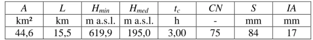
assessed through a terrain analysis of a 20 m resolution DEM, are listed in table 1. 15
As proposed by Giandotti (1934), who analysed a number of natural floods in Italy, the time 16
of concentration tc (h) can be estimated by equation (14) as a function of the catchment area A
17
(km2), the main reach length L (km) and the elevation drop, expressed as the difference 18
between the average elevation Have (m a.s.l.) and the minimum elevation Hmin (m a.s.l.).
19 min 8 . 0 5 . 1 4 H H L A t ave c (14) 20
The infiltration capacity is moderately low and soils can be averagely classified in hydrologic 21
group C, according to the CN-SCS method (Soil Conservation Service, 1972). The land cover 22
consists in woods in the upstream catchment which are progressively substituted by 23
agricultural parcels included into residential and industrial areas in the valley bottom. 24
The CN value is reported in table 1, along with the soil moisture deficit at the time runoff 1
begins S and the initial abstraction IA, evaluated by using standard CN-SCS criteria for the 2
average moisture condition AMC II. 3
The watershed precipitation regime is sub-alpine with two maximums, spring and autumn, 4
and two minimums, winter and summer, while the annual average rainfall depth is about 900 5
mm. During summer, short duration and high intensity storms separated by long dry weather 6
periods occur. On the contrary, longer but less intense precipitations feature the wet seasons. 7
The meteorological input to the different procedures was represented by a 45 year long time 8
series of rainfall observations recorded every 30 minutes at the ITAS Pastori raingauge (1949-9
1993), located in Brescia, a few kilometres south of the watershed. 10
Two routing basins, one on-line and one off-line, were hypothesized to obtain diverse peak 11
attenuation efficiencies. Storage volumes and outlet control structures were preliminary sized 12
by means of a conventional design storm method. Long term performances were then 13
estimated by continuous approaches. 14
3.1 Basin design
15
The design storm method was firstly based on a lumped hydrological model to derive inflow 16
hydrographs for varying return periods. In the Italian hydrologic practice, ddf curves are 17
usually expressed as simple monomial relationships (15), whose parameters a (mm/hn) and n 18
generally depend on the return period T (years). 19 n T T T t a d v , (15) 20
Nevertheless, when the rainfall volume variability shows scaling properties (Burlando and 21
Rosso, 1996) and is suitably represented by Gumbel distributions for any durations, as in this 22
case, equation (15) can be written in the terms of equation (16) (Bacchi et al., 1995). 23
tT tn T T CV v v 1 ln ln 5772 . 0 283 . 1 1 1 , (16) 1
In this formulation the exponent n is constant and the coefficient a is directly expressed as a 2
function of the return period T by two sample statistics: CV is the variation coefficient mean 3
of the maximum annual rainfall volume samples recorded for different durations t (h) (usually 4
1 h, 3 h, 6 h, 12 h and 24 h), while v1 (mm) is the mean maximum annual hourly rainfall
5
volume. Ddf parameter values estimated for the Brescia raingauge are: 0.33, 0.36 and 28.3 6
mm for n, CV and v1, respectively.
7
The point precipitation was converted into areal precipitation by the area reduction factor (17) 8
proposed by Moisello and Papiri (1986) for rain fields North Italy, when the catchment area A 9
(km2) ranges between 5 and 800 km2 and the duration t between 0.15 and 12 h. 10 , 1 exp
2.472 0.242 0.6 exp0.643 0.235
A T A A t r (17) 11The design rainfall pattern was thus developed according to the Chicago method (Akan and 12
Houghtalen, 2003), by setting the storm duration equal to twice the catchment time of 13
concentration. This choice was intended to match two opposite design targets: on one hand, to 14
have a significant flood volume, on the other hand, to maintain high peak flow rates. Since the 15
area reduction factor (17) depends on the rainfall duration and the intensity varies inside the 16
wet weather period, rainfall volumes for partial durations were deduced from the aerial ddf 17
curve, given by the product of (16) and (17), so that short duration intensities were reduced 18
more than the lower ones. 19
Hydrological losses were computed by means of the SCS-CN procedure under average 20
antecedent moisture conditions (AMC II), since extreme conditions are considered to yield 21
unreasonable large, or low, runoff volumes when applied within a design storm procedure. 22
The rainfall excess was finally routed by a Nash conceptual scheme (Nash, 1957) consisting 23
in a combination of two linear reservoirs to obtain the outlet discharge. The storage constant 24
kN was assessed through equation (18), that originates from a similitude between the
1
instantaneous unitary hydrograph peak of the Nash method and that of the kinematic method, 2
if a triangular shape is assumed (Bacchi et al., 1989). In such an equation, ni is the number of
3
reservoirs, (.) the complete gamma function and tc the catchment time of concentration given
4 by equation (14): 5
c i n n i N t n e n k i i 2 1 1 1 . (18) 6According to Akan (1989), various design hydrographs related to return periods rising from 5 7
years to 100 years were derived and utilized as inflow to simulate the basin behaviour. To do 8
so, hydraulic models of the routing reservoirs were developed for the connection scheme 9
illustrated in figure 5 a), for the on-line case, and in figure 5 b), for the off-line one. 10
In the former, an embankment crossing the stream bed and directly intercepting the natural 11
flow is employed to delimitate an open pond. Outlet orifices and a spillway were set to 12
provide increasing discharge capacity with the water stage. In the latter, the stream flow is 13
diverted into an analogous open pond by a side weir combined with a gate. The captured 14
runoff is discharged towards the downstream reach by orifices, a spillway and a pump system, 15
to facilitate the emptying process for very low stages. Storage volumes and outlet discharge 16
curves were defined by a trial process in which they were changed step by step to obtain a 17
desired routing efficiency (19). 18 pi po pi q q q (19) 19
The storage capacity was finally evaluated in 400000 m3 for both the connection types, the 20
threshold discharge qS in 45 m3/s, and the basin storage constants kS were established in 1.1 h,
21
for the on-line basin, and in 3.1 h, for the off-line one. Storage constants were estimated as the 22
ratio between the stored volume and the outlet discharge corresponding to the filling 23
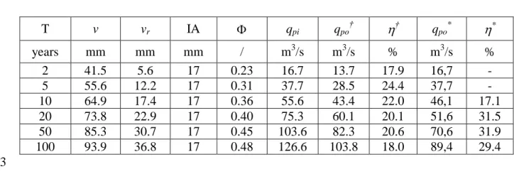
condition. With reference to the previously defined variables, table 2 reports a synthesis of the 24
hydrologic balances and the routing efficiencies assessed for the analysed return periods. The 1
well-known greater effectiveness of the off-line basin allowed to maintain an efficiency value 2
of about 31%, for peak rates significantly larger than the threshold qS, while a minor value of
3
about 20% was admitted for the on-line storage solution. 4
3.2 Continuous simulations
5
Continuous simulations of the rainfall-runoff transformation and routing processes occurring 6
in the watershed-basin system were performed by means of the previously described model, 7
in which the observed precipitation time series was employed as meteorological input. Some 8
adaptations were however necessary to pass from the event based analysis to the continuous 9
simulation. 10
Firstly, the reduction of the point precipitation to the area was carried out by using variable 11
factors inside the same storm by considering greater durations centred on the peak intensities. 12
Secondly, the SCS-CN method can be implemented in this kind of modelling if the AMC 13
variability and the catchment moisture decay during dry weather periods are properly 14
accounted for (Mishra and Singh, 2004). Hence, during interevent periods, CN values were 15
updated with regard to the conventional antecedent precipitation index API5 and seasonal
16
AMC thresholds, while the residual moisture at the rainfall end was completely depleted 17
within five days by an exponential function. 18
The three simulation outputs were statistically analysed through individual event statistics 19
(IES), that is, the continuous series were separated in independent floods, detecting their peak 20
flow rates and counting their average annual number f. In order to ensure the consistency
21
with the analytical-probabilistic model, the minimum time between floods utilized for 22
separating the discharge series were equal to IETDs adopted for fitting the corresponding 23
probability functions. Thus, the experimental return period T was estimated by the expression 24
) 1 ( 1 Qp f F T (20) 1
The more conventional formulation basing on the maximum annual statistics actually gives 2
matching results when the return period is greater than 10:20 years. However, this estimate is 3
conceptually more correct and should be more reliable for the lower return periods. 4
3.3 Analytical probabilistic model calibration
5
The precipitation time series was separated in independent events by the discretization 6
thresholds IETD and IA. Bearing in mind the discussion regarding their physical meaning, 7
IETDs of 3 h, 4 h and 6 h were taken into consideration for the inflow discharge, the outflow 8
routed by an on-line basin and the outflow routed by an off-line basin, respectively. The first 9
value was assumed equal to the catchment time of concentration tc, while the others were
10
computed as the sum of this quantity and the storage constant kS, considered to be an index of
11
the average residence time of the stored runoff. By this choice, the initial condition of totally 12
empty storage volume, implicit in the routing scheme of Whycoff and Singh (1976) 13
implemented in the derivation procedure, is mostly satisfied when an independent event 14
occurs. 15
In this formulation the volume threshold of the discretization procedure must be equal to the 16
initial abstraction of the simplified hydrologic loss model (2). In addition, the analytical-17
probabilistic approach must operate in average conditions. Therefore, the threshold IA was set 18
equal to 17 mm, corresponding to AMC II, table 1. Indeed, because of its large value, the 19
latter parameter demonstrated to be dominating in the calibration of the derived cdfs, so that 20
variations in the IETD setting were not particularly relevant. 21
The scale parameters of the joint probability density function pVT (1) were then assessed
22
through the maximum likelihood criterion from the independent event samples, obtaining 23
16.8 mm for and 19.8 h for . The average annual number of storms s, required to convert
non exeedance probabilities (6), (11) and (13) in return period by equations analogous to (19), 1
was estimated as well. 2
However, as it was expected, the parameter with respect to which all derived distributions 3
proved to be more sensitive was the average runoff coefficient of equation (2). Being the 4
main objective of this work evaluating the discrepancies between continuous approaches, 5
their maximum consistency had to be ensured. Thus, the average runoff coefficient was 6
computed through hydrological simulations, comparing the simulated runoff volumes to the 7
rainfall portions exceeding the actual initial abstraction: a value of 0.32 was assessed. 8
3.4 Result and discussion
9
The first proof was aimed at verifying that the average annual number of floods f and of
10
storms s are equal. In fact, because of the adopted discretization criterion, all independent
11
storms are runoff producing and consequently issue a flood. As auspicated, matching 12
outcomes were obtained: a number of 4:6 floods per years were deduced for the defined IETD 13
range. Such values were considered to be reasonable for the flow regime of this kind of 14
natural catchment. 15
The frequency distributions of the peak inflow discharge qpi developed through continuous
16
approaches are represented in figure 6, along with the peak flow rates derived by the design 17
storm method. An overall satisfactory agreement is evidenced between the analytical-18
probabilistic curve and the continuous simulation statistics, especially when the return period 19
T rises over 2 years. In the interval 1:2 years, which is however out of interest even for the 20
smallest urban applications, discrepancies consist in an overestimation of the peak discharges. 21
This behaviour may be partly explained by the incapability of a triangular hydrograph to suit 22
the real flood patterns for very low flows, which should lead to a peak magnification. The 23
observation of the distribution graphs in figure 7 and 8 yield analogous considerations for the 24
The effectiveness both of the derived model formulation and of the calibration criteria is 1
therefore supported. In particular, i) the implementation of a variable stored volume in spite of 2
a constant storage capacity demonstrated to be extremely important to avoid performance 3
overestimations of the on-line basin when the return period ranges between 5:20 years, ii) the 4
introduction of the non exeedance probability PQs constrain is crucial to catch the general
5
behaviour of the off-line basin over the discharge qS.
6
However, in all the three cases, peak discharges derived by the design storm method show to 7
be realistic as well and, for 2 years return periods, to better match continuous simulations than 8
the analytical-probabilistic curves do. Nevertheless, continuous simulations evidenced that 9
AMC II, which was assumed for the hydrologic loss computation, is satisfied by only the 18% 10
of storms. This goodness must consequently be interpreted as an expected, but fortuitous, 11
compensation of errors. 12
4 Conclusions
13Although relevant simplifications in the representation of the probabilistic precipitation 14
structure and of the hydrologic processes were exploited, a practical analytical-probabilistic 15
method devoted to size routing basins has been herein derived. The study shows that the 16
method yields outcomes in satisfactory agreement with those of benchmarking continuous 17
simulations. 18
Such a model goodness has been achieved through some significant improvements in the 19
schematization of the device hydraulic behaviour, when the storage volume is supplied either 20
on-line or off-line. Moreover, since the model was tested with respect to a small-medium size 21
natural watershed, the possibility to employ analytical-probabilistic methodologies for 22
hydrologic applications concerning large spatial scales is supported. 23
When the discretization thresholds are chosen with regard to parameters featuring the 24
considered hydrologic-hydraulic phenomena, the proposed strategy appears to be efficacious 25
in keeping the derived model as simple as possible and evenly isolating events actually 1
independent for the device. In this particular context, the large value of the initial abstraction 2
IA allowed to generate floods having significant runoff volumes, while the value of the 3
interevent time definition IETD equal to the catchment-basin response time avoids the flood 4
overlapping and ensures that the basin is completely empty for any floods. 5
5 References
1[1] Andrés-Doménec I, Montanari A, Marco JB. Stochastic rainfall analysis for storm tank 2
performance evaluation. Hydrol Earth Syst Sci 2010;14(7):1221–1232. doi: 10.5194/hess-3
14-1221-2010. 4
[2] Adams BJ, Howard CDD. Design storm pathology. Can Water Resour J 5
1986;11(3):4955. doi:10.4296/cwrj1103049. 6
[3] Adams BJ, Fraser HG, Howard CDD, Hanafy MS. Meteorological data analysis for 7
drainage system design. J Environ Eng-ASCE 1986;112(5):82748. 8
doi:10.1061/(ASCE)0733-9372(1986)112:5(827). 9
[4] Adams BJ, Papa F. Urban stormwater management planning with analytical probabilistic 10
models. New York, NY: John Wiley & Sons; 2000. 11
[5] Akan AO. Detention pond sizing for multiple return periods. J Hydraul Eng-ASCE 12
1989;115(5):65064. doi:10.1061/(ASCE)0733-9429(1989)115:5(650). 13
[6] Akan AO, Houghtalen RJ. Urban hydrology, hydraulics and stormwater quality. 14
Hoboken, NJ: John Wiley & Sons; 2003. 15
[7] American Society of Civil Engineers, Water Environmental Federation. Urban runoff 16
quality management. Reston, VA: American Society of Civil Engineers; 1998. 17
[8] Bacchi B, Larcan E, Rosso R. Stima del fattore di attenuazione per la valutazione del 18
colmo di piena prodotto da piogge efficaci di durata finita ed intensità costante. 19
Ingegneria Sanitaria 1989;1:6-15. Italian 20
[9] Bacchi B, Mariani M, Ranzi R. Analisi delle piogge intense e forte intensità a scala 21
regionale: Pianura Padana, Valtellina e Orobie. DICATA Technical Report, Università di 22
Brescia, Brescia, 1995. Italian 23
[10] Bacchi B, Brath A, Maione U. Sul dimensionamento delle reti di drenaggio con la 24
metodologia dell’evento critico. Idrotecnica 1993;1:33–43. Italian. 25
[11] Bacchi B, Balistrocchi M, Grossi G. Proposal of a semi-probabilistic approach for 26
storage facility design. Urban Water J 2008;5(3):195–208. 27
doi:10.1080/15730620801980723. 28
[12] Balistrocchi M, Grossi G, Bacchi B. An analytical probabilistic model of the quality 29
efficiency of a sewer tank. Water Resour Res 2009;45, W12420:1–12. 30
doi:10.1029/2009WR007822. 31
[13] Balistrocchi M, Bacchi B. Modelling the statistical dependence of rainfall event variables 32
through copula functions. Hydrol Earth Sys Sciences 2011;15(6):1959–77. 33
doi:10.5194/hess-15-1959-2011. 34
[14] Bonta JV, Rao R. Factors affecting the identification of independent storm events. J. 35
Hydrol 1988;98(3-4):275–93. doi:10.1016/0022-1694(88)90018-2. 36
[15] Burlando P, Rosso R. Scaling and multiscaling models of depth-duration-frequency 1
curves for storm precipitation. J. Hydrol 1996;186(1-2):45–64. doi:10.1016/S0022-2
1694(96)03086-7. 3
[16] Chow VT, Maidment DR, Mays LW. Applied hydrology. Singapore, SG: McGraw-Hill; 4
1988. 5
[17] Cordova JR, Rodriguez-Iturbe I. On the probabilistic structure of storm surface runoff. 6
Water Resour Res 1985;21(5):755–63. doi:10.1029/WR021i005p00755. 7
[18] Directive 2007/60/EC of the European parliament and of the Council on the assessment 8
and the management of flood risks (23 Oct. 2007). 9
[19] De Michele C, Salvadori G. On the derived flood frequency distribution: analytical 10
formulation and the influence of antecedent soil moisture condition. J Hydrol 11
2002;262(14):24558. doi:10.1016/S0022-1694(02)00025-2. 12
[20] De Michele C, Salvadori G, Canossi M, Petaccia A, Rosso R. Bivariate statistical 13
approach to check adequacy of dam spillway. J Hydrol Eng 2005;10(1):507. 14
doi:10.1061/(ASCE)1084-0699(2005)10:1(50). 15
[21] Diaz-Granados MA, Valdes JB, Bras RL. (1984), A physically based flood frequency 16
distribution. Water Resour Res 1984;20(7):995–1002. doi:10.1029/WR020i007p00995. 17
[22] Dunkerley D. Identifying individual rain events from pluviograph records: a review with 18
analysis of data from an Australian dryland site. Hydrol Process 2008;22(26):5024–36. 19
doi:10.1002/hyp.7122. 20
[23] Eagleson SP. Dynamics of flood frequency. Water Resour. Res 1972;8(4):878–98. 21
doi:10.1029/WR008i004p00878. 22
[24] Giandotti M. Previsione delle piene e delle magre dei corsi d’acqua. Rome, IT: Ministero 23
dei Lavori Pubblici, Servizio Idrografico Italiano; 1934. 24
[25] Goel NK, Seth SM, Chandra S. Multivariate modeling of flood flows. J Hydraul Eng-25
ASCE 1998;124(2):14655. doi:10.1061/(ASCE)0733-9429(1998)124:2(146). 26
[26] Grimaldi S, Serinaldi F. Asymmetric copula in multivariate flood frequency analysis. 27
Adv Water Resour 2006;29(8):115567. doi:10.1016/j.advwatres.2005.09.005. 28
[27] Guo Y, Adams BJ. Hydrologic analysis of urban catchments with event-based 29
probabilistic models: 2. Peak discharge rate. Water Resour Res 1998;34(12):343343. 30
doi:10.1029/98WR02448. 31
[28] Guo Y, Adams BJ. An analytical probabilistic approach to sizing flood control detention 32
facilities. Water Resour Res 1999;35(8):245768. doi:10.1029/1999WR900125. 33
[29] Hong Y-M. Graphical estimation of detention pond volume for rainfall of short duration. 34
J Hydrol-Env Res 2008;2(2):10917. doi:10.1016/j.jher.2008.06.003. 35
[30] Kao SC, Govindaraju RS. A bivariate frequency analysis of extreme rainfall with 1
implications for design. J Geophys Res 2007;112(XX):D13119. 2
doi:10.1029/2007JD008522. 3
[31] Krstanovic PF, Singh VP. A multivariate stochastic flood analysis using entropy. In: 4
Singh VP, editor. Hydrologic frequency modelling. Dordrecht, NL: Reidel, 1987. p. 5
51539. 6
[32] Lynch JA, Corbett ES, Sopper WE. Effects of the antecedent soil moisture on stormflow 7
volumes and timing. In: Beven KJ, editor. Streamflow generation processes. Benchmark 8
papers in hydrology, 1. Wallingford, UK: International Association of Hydrological 9
Sciences (IAHS), 2006. p. 32435. 10
[33] Maglionico M 11
[34] Mambretti S. [Practical methods for routing tank design in urban environment] 12
[Dissertation]. Milan (IT): Milan Polytechnic; 1991. Italian. 13
[35] Marsalek J. Synthesized and historical storms for urban drainage design. Proceedings of 14
the 1st International Conference on Urban Storm Drainage; 1978; University of 15
Southampton, Chichester, UK. 16
[36] Mishra SK, Singh VP. Long-term hydrological simulation based on the Soil 17
Conservation Service curve number. Hydrol Process 2004;18(7):1291313. 18
doi:10.1002/hyp.1344. 19
[37] Nelsen RB. An introduction to copulas. 2nd ed. New York: Springer; 2006. 20
[38] Papiri S, Moncalvo M, Valcher P. Sul dimensionamento idraulico delle vasche volano a 21
servizio delle reti di drenaggio urbano. Proceedings of the Conference in Memory of 22
Carlo Cao; 1998; University of Cagliari, Cagliari, IT. 23
[39] Quader A, Guo Y. Peak discharge estimation using analytical probabilistic and design 24
storm approaches. J Hydrol Eng 2006;11(1):4654. doi:10.1061/(ASCE)1084-25
0699(2006)11:1(46). 26
[40] Restrepo-Posada PJ, Eagleson, PS. Identification of independent rainstorms. J Hydrol 27
1982;55(1−4):303–19. doi:10.1016/0022-1694(82)90136-6. 28
[41] Sivapalan M, Wood EF, Beven KJ. On hydrologic similarity 3, a dimensionless flood 29
frequency model using a generalized geomorphic unit hydrograph and partial area runoff 30
generation. Water Resour Res 1990;26(1):4358. doi:10.1029/WR026i001p00043. 31
[42] Soil Conservation Service. Urban hydrology for small watershed, tech. rep. n. 55. 32
Washington: US Department of Agriculture; 1975. 33
[43] Urbonas BR, Stahre P. Stormwater best management practices and detention for water 34
quality, drainage and CSO management. Englewood Cliffs, NJ: Prentice Hall; 1993. 35
[44] Urbonas BR, Doerfer JT. Master planning for stream protection in urban watersheds. 36
Water Sci Technol 2005;51(2):23947. 37
[45] US Environmental Protection Agency. Low impact development (LID), a literature 1
review (EPA-841-B-00-005). Washington, DC: US Environmental Protection Agency, 2
Office of Water; 2000. 3
[46] Walesh SG. Urban surface water management. New York, NY: John Wiley & Sons; 4
1989. 5
[47] Wycoff RL, Singh UP. Preliminary hydrologic design of small flood detention reservoirs. 6
Water Resour Bull 1976;12(2):33749. 7
[48] Yue S. The bivariate lognormal distribution to model a multivariate flood episode. 8 Hydrol Process 2000;14(14):57588. 9 doi:10.1002/1099-1085(20001015)14:14<2575::AID-HYP115>3.0.CO;2-L 10 11 12
TABLES
1Table 1: main hydrological characteristics of the Garza watershed. 2 A L Hmin Hmed tc CN S IA km² km m a.s.l. m a.s.l. h - mm mm 44,6 15,5 619,9 195,0 3,00 75 84 17 3 4
Table 2: main hydrologic characteristics of the design storm events employed to size the on-1
line† and the off-line* basins. 2 T v vr IA qpi qpo† † qpo* * years mm mm mm / m3/s m3/s % m3/s % 2 41.5 5.6 17 0.23 16.7 13.7 17.9 16,7 - 5 55.6 12.2 17 0.31 37.7 28.5 24.4 37,7 - 10 64.9 17.4 17 0.36 55.6 43.4 22.0 46,1 17.1 20 73.8 22.9 17 0.40 75.3 60.1 20.1 51,6 31.5 50 85.3 30.7 17 0.45 103.6 82.3 20.6 70,6 31.9 100 93.9 36.8 17 0.48 126.6 103.8 18.0 89,4 29.4 3 4 5
FIGURE CAPTIONS
1Figure 1: Simplified hydrographs associated with the routing process (adapted from Wycoff 2
& Singh, 1976). 3
Figure 2: integration domain for deriving peak inflow rate distribution. 4
Figure 3: integration domain for deriving peak outflow rate distribution for on line basins. 5
Figure 4: location and DEM of the Garza stream catchment. 6
Figure 5: connection scheme of the storage volume to the stream riverbed a) on-line b) off-7
line. 8
Figure 6: distributions of the peak inflow rates (CS IES: continuous simulation individual 9
event statistics, DSM: design storm method; APM: analytical-probabilistic method). 10
Figure 7: distributions of the peak outflow rates for on line basins (CS IES: continuous 11
simulation individual event statistics, DSM: design storm method; APM: analytical-12
probabilistic method). 13
Figure 8: distributions of the peak outflow rates for off line basins (CS IES: continuous 14
simulation individual event statistics, DSM: design storm method; APM: analytical-15 probabilistic method). 16 17 18 19 20
FIGURES
1 2 Figure 1 3 41
Figure 2 2
3 4
1
Figure 3 2
1 Figure 4 2 3 4 5
1
Figure 5 2
3 4
1
Figure 6 2
1 Figure 7 2 3 4 5
1
Figure 8 2