Equilibrium Selection, Similarity Judgments and the “Nothing to Gain/Nothing to Lose” Effect
Jonathan W. Leland
University of Trento and the National Science Foundation1
September 14, 2006 Abstract
Rubinstein (1988, 2003) and Leland (1994, 1998, 2001, 2002) have shown that choices based on similarity judgments will account for the vast majority of observed
violations of expected and discounted utility. In this paper, I show that such judgments also explain which equilibria will be selected in single-shot games with
multiple equilibria, predict circumstances in which non-equilibria outcomes may predominate in such games, and predict circumstances in which specific pure strategy
outcomes will predominate in games with no pure strategy equilibria.
1I would like to thank David Levine and Axel Leijonhufvud for provided invaluable feedback on my work on the topic of this paper. Oxana Tokarchuk provided outstanding research assistance and Marco Tecilla provided expert assistance in implementing the experiments discussed in this paper. Errors are the responsibility of the author. This research was supported by a ‘Rientro dei cervelli’ Research Fellowship from the Italian Ministry for Education, University and Research (MIUR). Views
expressed do not necessarily represent the views the National Science Foundation or the United States government.
“Games with multiple equilibria require coordination…. Predicting which of the many equilibria will be selected is perhaps the most difficult problem in game
theory.” (Camerer, 2003, pp. 336)
Introduction
A frequently encountered challenge in game theory involves predicting how agents will play in games with multiple equilibria. Theorists have proposed a number of deductive principles – payoff dominance, risk dominance, security-mindedness - people might use to winnow down the available options. None of these criteria consistently explain which equilibrium subjects select in experimental settings. In this paper, I take a different tack to address the question of equilibrium selection. Specifically, I show that if people base their strategy choices on judgments regarding the similarity or dissimilarity of game payoffs, along lines proposed by Rubinstein (1988, 2003) and Leland (1994, 1998, 2001, 2002) to explain why people violate the axioms of expected utility and discounted utility, then in single-shot games, they may systematically select one strategy over another as a function of the relative magnitude of game payoffs.2
I begin with a short discussion of the consequences of choosing between risky and intertemporal prospects based on similarity judgments and identify the intuition driving these predictions – an intuition referred to as the “nothing to gain / nothing to lose” effect. Next, I propose a similarity-based procedure whereby individuals choose strategies in simple 2x2 games. Strategy choices recommended by this procedure are sensitive to the relative magnitude of game payoffs. In the context of games for which there are multiple equilibria, this procedure implies that for certain configurations of payoffs, players may perceive that there is “nothing to lose” by
choosing the strategy corresponding to payoff dominance. For other payoff configurations, there may appear to be “nothing to gain” by choosing that strategy in which case the strategy corresponding to security-mindedness will be selected. Should one player face a payoff configuration for which there appears to be “nothing to lose” by choosing the strategy corresponding to payoff dominance and the other player a configuration suggesting the security-minded strategy be selected, the model predicts that the result of the game will be one of the non-equilibrium outcomes.
In games involving pure conflict in which there are no pure strategy equilibria, the procedure implies that certain payoff configurations will, nonetheless, result in specific pure strategy outcomes predominating. Finally, the procedure implies that theoretically inconsequential re-framing of games may influence subjects’ strategy choices and the resulting game outcomes. Data confirming all these predictions is presented.
Similarity Judgments and the “Nothing to Gain / Nothing to Lose” Effect
Imagine giving people a choice between the lottery R:{ $10, .1, $0, .9 } and its expected value EV{R}= $1 and a choice between the lottery R:{ $10, .9, $0, .1 } and its expected value EV{R}= $9. We would not be surprised if they chose the lottery in the first case but the expected value in the second. Though plausible, this pair of choices is inconsistent with the standard assumption of risk aversion. However, both choices follow in a straight-forward manner if people choose based upon similarity judgments along lines suggested by Rubinstein (1988, 2003) and Leland (1994, 1998, 2001, 2002).3 To illustrate, suppose that between simple lotteries of the form,
3 Related work was done early on by Tversky (1969) and Montgomery (1983), and more recently by psychologists (e.g., Medin, Goldstone and Markman (1995), Markman and Medin (1995), Mellers and Biagini (1994)
Gonzalez-R:{ $10, p, $0, 1-p }, and their corresponding expected values, S:{EV[R]}, agents recognize that there are circumstances, to occur with probability p, in which the lottery will yield $10 while the certain alternative yields EV{R} and other circumstances, occurring with probability 1-p, in which the lottery yields $0 while the alternative course of action again yields EV{R}. If so, then we can think of agents as representing the choice as shown below.
R: { $10 , p ; $0 , 1-p }
S: { EV{R} , p ; EV{R} , 1-p }
To choose between these alternatives assume agents compare prizes $10 and EV{R} and their associated probabilities of occurrence, p and p, and then the prizes $0 and EV{R} and their associated probabilities, 1-p and 1-p, where all comparisons concern whether the values appear similar or dissimilar. For each pair of comparisons, agents decide whether the pair 1) “favor” one alternative over another (e.g., when one alternative offers a dissimilar and better prize at dissimilar and greater or similar probability), 2) are “inconclusive” (e.g., when one lottery offers a dissimilar and better prize but the other offers a good prize at dissimilar and greater probability ) or, 3) are “inconsequential” (e.g., when both lotteries offer similar prizes at similar probabilities). Assume further that players choose one option over the other if it is favored in some comparisons and not disfavored in any and at random otherwise.4 For
choices between R and S evaluated in this manner, when p is small and thus EV{R} close to $0, $1 for example, the risky alternative R will be preferred to the extent that if offers noticeably better prize (e.g., $10 versus $1) at similar, indeed identical, probability and a worst outcome $0 similar to EV{R}, again at similar (equal)
Vallejo (2002)) as well as economists (e.g., Azipurtha et al (1993), Buchena and Zelberman (1995), and Loomes (2006)).
probability. In such cases, there appears to be “nothing to lose” by gambling. As p increases, we reach a point where either $10 appears dissimilar to EV{R} and EV{R} dissimilar to $0 or $10 similar to EV{R} and EV{R} similar to $0. In these cases, the comparisons are uninformative to the extent that either one favors R and one favors S or both are inconsequential. For sufficient increases in p, however, the safe alternative S will be preferred to the extent that it offers a prize EV{R} that appears similar to the best possible outcome in R (e.g., $10 versus $9) at similar probability (the first paired comparison is “inconsequential”) and an outcome noticeably superior to the worst outcome in R (e.g., $9 versus $0) at similar probability – a comparison favoring S. Here there appears to be “nothing to gain” by gambling.
To summarize, let the binary relations >x and > p reading "greater than and dissimilar" be strict partial orders (asymmetric and transitive) on consequences and probabilities, respectively. As such, the similarity relations, ~ x and ~p, defined by > x and > p are symmetric but not necessarily transitive in that for some prizes x f >x g > x h, x f ~ x x g, x g ~ x x h but x f > x x h with the same being possible for probabilities. Given this notation, for choices between a lottery and its expected value, as p
increases, the predictions following from the “nothing to gain / nothing to lose” effect are as follows. Table 1 $10 >x EV{R}, EV{R} ~x $0 $10 >x EV{R}, EV{R}>x $0, $10 ~x EV{R}, EV{R} ~x $0 $10 ~x EV{R}, EV{R} >x $0 R ? S ntl ntg Increasing p
While extremely simple, maybe simple-minded, this type of reasoning about which components across alternative options appear similar and which appear
dissimilar enables us to explain the vast majority of instances in which people systematically violate the axioms of expected utility.
As but one example, consider the lotteries shown below: S:{ 3000, .90 ; 0, .10 } S':{ 3000, .02 ; 0, .98 } R:{ 6000, .45 ; 0, .55 } R':{ 6000, .01 ; 0, .99 }
Given these choices people tend to choose S over R but R’ over S’. This choice pattern constitutes what is known as the “common ratio” violation of the independence axiom. That the choices are inconsistent with independence follows from the fact that S’ and R’ are just 1/45th chances of S and R, respectively.
To see how these choices are explained by similarity judgements, consider first the choice between S’ and R’. Given these alternatives, agents first compare $3000 with $6000 and .02 with .01 and then compare $0 with itself and .98 with .99. In the first paired comparison assume that $6000 appears dissimilar and greater than $3000 and that .02 appears similar to .01. If so, then the first paired comparison "favors" R' to the extent that it offers a noticeably better prize at similar probability. In the second paired comparison, the lotteries offer the same worst prize, $0, at similar probability, .99 ~p .98, in which case the comparison is deemed "inconsequential".
Thus it appears there is “nothing to lose” by choosing the risky alternative to the extent it offers a noticeably better prize at similar probability and the same worst outcome at similar probability.
Scaling lottery probabilities up while holding their ratio constant may eventually make them appear dissimilar. If so, then in choosing between R and S agents will perceive $6000 >x $3000 and .90 >p .45 in which case the first paired
comparison will be judged "inconclusive" - R offers a noticeably better prize but S offers a good prize at noticeably higher probability. The second paired comparison
will, however, "favor" S as R offers a similar worst prize ($0 ~x $0) at noticeably
higher probability (.55 >p .10). As such, S will be selected as it is favored in at least
one paired comparison and not disfavored in any others. Thus, as the probabilities of the non-zero outcomes rise in common ratio type lotteries, the predictions that follow if people base their choices on similarity judgements can be summarized as follows. Table 2 $6000 >x 3000, .02 ~p .01 $0 ~x $0, .99 ~p .98 $6000 >x 3000, .90 >p .45 $0 ~x $0, .10 >p .55 R S ntl Increasing p
Identical logic allows us to explain anomalies in intertemporal choice. Consider, for example, the choices between intertemporal prospects
S(maller)S(ooner)1 and L(arger)L(ater)2 and SS11 and LL12 below:
SS1 :{ $20 , 1 week } SS11 :{ $20 , 11 weeks }
LL2:{ $25 , 2 weeks } LL12:{ $25 , 12 weeks }
Individuals indifferent between SS1 and LL2 tend to strictly prefer LL12 to SS11
– a finding referred to as the “common difference” effect. Given the choice between SS1 and LL2 , individuals perceiving $25 as dissimilar and greater than $20 and a 2
week delay as dissimilar and worse than a 1 week delay, will conclude that the paired comparison is “inconclusive” and choose at random. However, if deferring both payoffs a constant amount into the future makes the delays appear similar (i.e. 12 weeks delay appears similar to 11 weeks delay), but $25 still appears dissimilar to $20, they will choose LL12 over SS11 since there appears to be “nothing to lose” by
waiting an additional week for a noticeably better payoff.5 Letting >t and ~ t denote
“dissimilar and greater” and “similar” time periods, respectively, these predictions can be summarized as follows: Table 3 $25 >x 20, 2 >t 1 $25 >x 20, 12 ~t 11 ? LL ntl Increasing t
The Nothing to Gain / Nothing to Lose Effect and Behavior in Games We are now in a position to consider what decisions based on similarity judgments might imply in the context of single-shot games. For this purpose, consider the following generic 2x2 game.
Figure 1
L R
Player 1 U a, w b, x
D c, y d, z
Given such a game, suppose that the players reason as follows:
1) Do I have a dominating strategy? For this purpose, assume Player 1 (2) first compares his payoffs a and c (w and x) under the assumption that the other player has chosen L (U) and then compares b and d (y and z) under the assumption that the other player has chosen R (D). 6 If a dominant
strategy is identified, it is selected: otherwise,
2) Do I have a dominating strategy given similar and dissimilar payoffs? For this purpose, Player 1 (with an analogous procedure for Player 2) again
6 You might think of the assumption that agents consider their own payoffs first as an assumption that we are dealing with the most basic, or maybe base, types of players in classification schemes discussed by Costa Gomes, Crawford and Broseta (2001) and Camerer, Ho, and Chong (2004).We will explore the consequences of
compares his payoffs a and c assuming Player 2 has chosen L and b and d assuming Player 2 has chosen R. Here, however, if a and c and/or b and d appear similar, Player 1 deems that comparison “Inconsequential” and bases his decision only on the other payoff comparison or, if both are inconsequential, continues to Step 3. If this process identifies a strategy which is dominant in similarity, it is selected: otherwise,
3) Does the other player have a dominating strategy? Here the process in Step 1 is repeated although now the players apply the reasoning to the other player’s payoffs. If the player concludes that the other has a dominant strategy, he best responds to that strategy: otherwise,
4) Does the other player have a dominating strategy given similar and dissimilar payoffs. Here the process in Step 2 is repeated although now the players apply the reasoning to the other player’s payoffs. If the player concludes that the other has a dominant strategy in similarity, he best responds to that strategy: otherwise,
5) Employ some other criterion for deciding (e.g., choose at random.)
The Role of Similarity Judgments in Coordination Games
Now consider how this procedure would apply in the following generalized stag-hunt or assurance game shown in abstract form below where Player 1 has payoffs h(igh), m(edium) and l(ow), and Player 2 has payoffs t(op), c(enter) and b(ottom):
Figure 2
L R
Player 1 U h, t l, c
In this game, there is no dominating strategy for Player 1 and, since the payoff ordering facing Player 2 is the same, no dominating strategy for Player 2. There are, however, two equilibria in pure strategies, UL and DR, as well as one mixed strategy. Both players would prefer the pareto optimal equilibrium UL to the pareto dominated one DR. UL is, however, riskier in the sense that if either player plays the strategy corresponding to the pareto dominant equilibrium, and the other player fails to do so, the first player incurs a loss of l (b), whereas if players choose the strategies
corresponding to the deficient equilibrium they are assured the intermediate payoff of m (c). Given this tension the question is, “Which of the pure strategy equilibria will players choose, if either?” Three criteria have been widely proposed as means whereby agents decide in favor of one equilibrium over another.
One criterion proposed in the literature is “payoff dominance.” It requires that players choose the equilibrium offering all players their highest payoff. By this criterion, row and column players should play U and L, respectively, and irrespective of the relative magnitudes of the payoffs – only the ordering of the payoffs matters.
A second possibility is that people are security-minded and choose the strategy that minimizes the worst possible payoff they might get. Players following this criterion will choose their maximin strategies resulting in the equilibrium DR. Here again, only the relative magnitudes of the payoffs matter.
A third criterion for equilibrium selection is “risk dominance.” A risk
dominant equilibrium is one that jointly minimizes the losses incurred by players as a consequence of unilaterally deviating from their equilibrium strategy. The risk
dominant strategy corresponds to the one that maximizes the Nash product of the players “own deviation” losses. As such, in contrast to payoff dominance and
security-mindedness, the strategy recommended by risk dominance depends not only on the ordering of the payoffs but also their relative magnitude.
As an empirical matter, none of these three selection criteria have proven very successful at explaining behavior observed in games involving multiple equilibria.7
With this in mind, consider how an individual employing the process described in the prior section would play this type of game. Given that there are no dominating
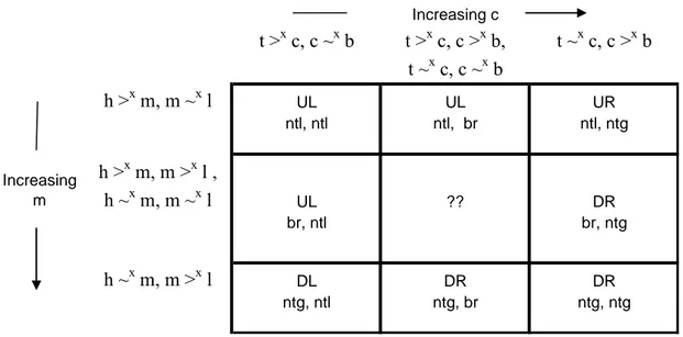
strategies in this game, players would proceed to the second step in the procedure and attempt to see whether there is a dominant alternative in similarity. Given the payoffs compared by each player, players might maintain any of 5 possible configurations of similarity and dissimilarity perceptions. The one where the best and worst outcome are similar is uninteresting and will henceforth be ignored. The other four are shown along the left and upper borders in Table 4 ordered for values of the intermediate payoffs m and c varying from small to large.
Table 4 t >x c, c ~x b t >x c, c >x b, t ~x c, c ~x b t ~x c, c >x b h >x m, m ~x l UL UL UR ntl, ntl ntl, br ntl, ntg Increasing m h >x m, m >x l , h ~x m, m ~x l UL ?? DR br, ntl br, ntg h ~x m, m >x l DL DR DR ntg, ntl ntg, br ntg, ntg Increasing c
The consequences of choosing based on similarity judgments are shown in the interior cells in the table. To see how these predictions arise, assume to begin that
7 See Camerer (2003) and Haruvy and Stahl (2004) for summaries of the evidence.
Player 2 perceives t(op) as dissimilar to c(enter) and c as similar to b(ottom) (i.e., the cases in the first column of Table 1) as would be the case if the center prize was as close in value to the bottom prize as possible. For this configuration of similarity perceptions, it will appear to Player 2 that there is “nothing to lose” by choosing L as it offers a noticeably better outcome than R, t versus c, in the first comparison made whereas R offers an outcome, c, similar to the worst outcome in L in the second comparison. Should Player 1 also perceive his high payoff as dissimilar to the middle one and it as similar to the low one, he will likewise conclude there is “nothing to lose” by choosing strategy U offering the highest payoff. In this case the payoff dominant equilibrium UL will be the outcome of the game. If, instead, Player 1 perceived h >x m and m >x l or h ~x m and m ~x l, as will eventually occur if m is
increased from its minimum value, the payoff comparisons are uninformative. In this case, Player 1 proceeds to Steps 3 and 4, tries to infer what Player 2 is going to do given the payoffs Player 2 faces, and best responds to that expected choice. Since, Player 2 doesn’t have a dominant strategy, Player 1 will attempt to infer whether he has a dominating strategy in similarity. Assume here, and throughout the remainder of the paper, that players share perceptions as to when payoffs are similar or
dissimilar. If so, Player 1 will correctly anticipate that Player 2 is going to choose L and best respond by choosing U. Once again, the payoff dominant equilibrium UL will be the outcome of the game. For continued increases in m, Player 1 will eventually perceive h(igh) as similar to m(edium) and m(edium) as dissimilar to l(ow), at which point he will feel there is “nothing to gain” by choosing the strategy corresponding to the payoff dominant equilibrium and play the security-minded strategy D instead. Now the outcome of the game will be the non-equilibrium
same logic. As indicated reading across the rows, down the columns and along the diagonal in the table, as the value of the intermediate payoff varies from low to high, players move from perceiving “nothing to lose” by choosing the higher payoff – higher variance option to perceiving that there is “nothing to gain” by doing so or, more formally:
Prediction 1: Given a 2x2 stag-hunt game with payoffs as configured in Figure 2, strategy choice will shift from U (L) to D (R) as the value of the intermediate payoff m (c ) varies from its minimum to its maximum.
To test this prediction and its associated implications regarding which outcome of a game should predominate, 76 student subjects participated in an experiment conducted at the University of Trento in Italy. The experiment consisted of three parts. 8 In the first part, subjects played 9 games. In each game, subjects were
randomly and anonymously matched with another participant in the experiment. In each game, subjects either chose between playing U(p) or D(own) or between L(eft) and (Right). All questions were presented in the format shown below.
If Other chooses L and you choose U You receive 8.00 and Other receives 8.00
D 5.00 2.00
If Other chooses R and you choose U You receive 2.00 and Other receives 5.00
D 5.00 5.00
Five of the questions were generalized stag-hunt games. Three were a generalized form of the matching pennies game. A final game, also a stag-hunt, tested whether play is subject to framing effects. The order of the first eight games was randomized
8 The second and third sets of questions presented to subjects involved binary choices between intertemporal and risky prospects, respectively.
subject to the constraint that a game of one type was never followed by a game of the identical type. The game testing for framing effects was always played last as it involved a change in instructions. Payoffs corresponding to the U or D and L or R label in each game also alternated at random. Subjects were told before the beginning of the experiment that at the end of the experimental session, one of the games would be selected at random and they would receive the payoff for that game resulting from their strategy choice and that of the individual with whom they were paired. Possible payoffs from this game ranged from 1.20 to 8 euro.
The five stag-hunt games are shown in Table 5. The upper matrix shows the payoff values for each game and the lower matrix the experimental results and equilibrium frequencies predicted based on players’ responses.
Table 5 L R Player 1 U 8.00, 8.00 2.00, 2.10 D 2.10, 2.00 2.10, 2.10 L R Player 1 U 8.00, 8.00 2.00, 5.00 D 5.00, 2.00 5.00, 5.00 Player 2 Player 1 L R L R L R U 8.00, 8.00 2.00, 2.10 U 8.00, 8.00 2.00, 5,00 Player 1 U 8.00, 8.00 2.00, 7.90 D 7.90, 2.00 7.90, 2.10 D 7,90, 2.00 7,90, 5.00 D 7.90, 2.00 7.90, 7.90 L R Player 1 U 95% 3% 37 (97%) D 3% 0% 1 (3%) 37 (97%) 1 (3%) L R Player 1 U 32% 15% 18 (47%) D 36% 17% 20 (53%) 26 (68%) 12 (32%) Player 2 Player 1 L R L R L R U 41% 4% 17 (45%) U 15% 14% 11 (29%) Player 1 U 13% 24% 14 (37%) D 51% 4% 21 (55%) D 37% 34% 27 (71%) D 22% 42% 24 (63%) 35 (92%) 3 (8%) 20(53%) 18 (47%) 13 (34%) 25 (66%)
III-I III-II III-III
Player 2 Player 2 I-I Player 2 II-II Increase m Player 2 III-III Player 2 Player 2 Increasing c Increase m Player 2 III-I III-II Player 2
II-I II-II II-III
I-I I-II I-III
In game I-I, m and c are set at minimum values of 2.1. This results in 97% of Player 1s playing U, 97% of Player 2s playing L, and the predominant predicted game outcome being UL (95%). In game III-I, the value of m is increased to 7.9. Consistent with Prediction 1, this increases the frequency with which Player 1s choose D from 3% to 55% (McNemar’s χ2
1df = 16.4091, p=.0001), leaves the
frequency with which Player 2s choose L (97% versus 92%) statistically unaffected (McNemar’s χ2
=.50, p= .4795 ), and results in the non-equilibrium outcome DL predominating at a predicted 51%.
Increasing m from 5 to 7.9 holding c fixed at 5 (i.e., moving from game II-II to game III-II) has a similar effect – the frequency with which Player 1s choose D
increases significantly from 53% to 71% (McNemar’s χ2
1df = 4 , p=.0455) while the
frequency with which Player 2s choose L (68% versus 53%) is statistically unaffected (McNemar’s χ2
= 2.083, p = .1489).
Returning to game III-I in which m is at its maximum of 7.9 and c at its minimum value of 2.1, if we now increase c to 5 (Game III-II) and then to 7.9 (game III-III) the frequency with which Player 2 chooses the security-minded strategy R rises from 8% to 47% to 66% as per Prediction 1. A Cochrane test evaluating differences among related proportions for Player 2 is significant (χ2
2df = 29.1538, p=
.0000). The difference in proportion between games III-I and III-II is significant (McNemar’s χ2
= 10.3158, p=.0013) while the difference between proportions in games III-II and III-III is just shy of significance (McNemar’s χ2
1df =3.2727, p =
.0704). The proportions of Player 1s choosing D across these three games (55%, 71% and 63%) differ insignificantly ((χ2
2df = 3.85714, p=.145356) as is to be expected
given the payoffs facing Player 1s didn’t change across these three games. Also as anticipated, the predominant outcome of the game predicted based on players’
strategy choices shifts away from the non-equilibrium outcome DL toward the equilibrium DR as c rises. Specifically, while in game III-I there are 51% DL outcomes implied by the Player 1 and Player 2 responses and only 4% DR outcomes implied, when c takes on the intermediate value of 5, the implied percentage of DL outcomes falls to 37% while the expected DR percentage rises to 34%. For c equal to 7.9 the results are even more extreme with the percentage of DL outcomes implied by subjects’ responses falling to 22% while the expected DR percentage rises to 42%.
Games I-I, II-II and III-III examine the effects of simultaneously increasing both m and c from 2.1 to 5 to 7.9. Once again, the proportion of D (R) choices
increases systematically from 3% to 53% to 63% for Player 1 (and 3% to 32% to 66% for Player 2.) A Cochrane test evaluating differences among related proportions for Player 1s and Player 2s combined as the game is symmetric is significant (χ2
2df =
66.63, p= .0000 ) as are tests for the difference in proportion between games I-I and II-II (McNemar’s χ2
1df =28.13, p= .0000 ) and between games II-II and III-III
(McNemar’s χ2
1df =12.57, p = .0004). Also as anticipated, the predominant outcome
of the game predicted based on players’ strategy choices shifts away from the payoff dominant equilibrium, UL, (from 95% to 32% to 13%) and toward the security-minded one, DR (from 0% to 17% to 42%) as m and c rise.
Table 6 summarizes how these results square with the predictions of the equilibrium selection criteria discussed earlier as well as with the hypothesis that subjects are playing their Nash mixed strategies where, for clarity, we consider only Games I-I, III-I and III-III for which the “nothing to gain / nothing to lose” effect predictions are strict.
Game I-I III-I III-III Predominant Eq. Predicted Based on
Player' Responses UL (95%) DL (51%) DR (42%)
Equilibrium Selection Criterion
Mixed Strategies DR 25% each UL
Payoff Dominance UL UL UL
Security-mindedness DR DR DR
Risk Dominance UL UL or DR DR
ntg/ntl UL DL DR
As indicated in the table, the predictions that follow from the hypothesis that players are employing Nash mixed strategies are exactly wrong. Of the selection criteria, payoff dominance predicts the choice of UL in all three games independent of the values of m and c while security-mindedness predicts DR in all three. As a
consequence, these selection criteria only predict the predominant outcome in one of the games correctly. Risk dominance performs best, correctly predicting the
predominant outcomes in games I-I and III-III. It cannot, however, account for the behavior observed in game III-I.9
Results similar to the ones reported above have been reported elsewhere in the literature. Rydval and Ortmann (2004), for example, report that in the game shown below on the left, 79% of subjects choose the strategy U, corresponding to payoff dominance, whereas in the game on the right only 44% do.
L R L R
Player 1 U (79%) 80, 80 10, 30 Player 1 U (44%) 80, 80 10, 50
D 30, 10 30, 30 D 50, 10 50,50
Player 2 Player 2
The difference between the game on the left and the one on the right is that the m=c payoff is increased from 30 to 50. According to Prediction 1, this should make
9 Moreover, when it works the reason is clear. When risk dominance predicts the payoff dominant equilibrium UL (in Game I-I) it is because the differences between the payoffs contributing to “nothing to lose” reasoning, h-m and t-c, are large so the Nash product associated with UL is large. Likewise, when it predicts the security-minded equilibrium DR, it is because differences between payoffs contributing to the perception that there is “nothing to gain,” m-l and c-b, are large so the Nash product of DR is large.
strategies associated with the payoff dominant equilibrium UL less attractive (since there appears to be “nothing to gain” by choosing U and L if 80 ~x 50) and those associated with the security-minded equilibrium DR more attractive (since there appears to be “something to lose” by not choosing D and R if 50 >x 10.)
Rydval and Ortmann (2005) interpret their findings as indicating the superiority of risk dominance over payoff dominance as a selection criterion.
However, other results argue against this interpretation in favor of the hypothesis that behavior is being generated by the “nothing to gain / nothing to lose” effect. To illustrate, consider the following games discussed by Keser and Vogt (2000).
L R L R U 70, 70 20, 5 28/48 (58%) U 140, 140 20, 5 35/36 (97%) D 5, 20 50, 50 D 5, 20 50, 50 Player 2 Player 2 Player 1 Player 1
Note that DR is the security-minded equilibrium in both these games whereas UL is payoff and risk dominant in both. The latter fact notwithstanding, in the game on the left, nearly half of subjects fail to choose according to risk dominance. Indeed, given the near 50:50 split in the first game, none of the three commonly proposed selection principles explain play here. If players perceive 70 as dissimilar and greater than 5 but also 50 as dissimilar and greater than 20, the approximate 50:50 split would be what we would expect if subjects were employing similarity judgments to make their strategy choices. 10
In the game on the right, the “h” and “t” payoffs of 70 have been increased to 140. While 50 may appear dissimilar to 20 in the context of payoffs of 70 and 5, if it
10 Interestingly, a slight majority of subjects (28/48) favor U. This is as it should be if people are choosing based on similarity as D cannot be recommended based on similarity judgments. For this to occur, 70 would have to appear similar to 5 but then 50 and 20 must be similar too at which point the choice is resolved at random. On the
appears similar to 20 in the presence of a much larger number, 140, there will appear to be “nothing to lose” by choosing the strategies corresponding to the payoff
dominant equilibrium.11 That this strategy also happens to be the risk dominant one is
an artifact.
Similarity Judgments in Games of Pure Conflict
The evidence presented above supports the hypothesis that people are basing their choices of strategies in simple 2x2 single-shot games on similarity judgments and not on some equilibrium selection principle nor randomization. To further substantiate this claim, we now consider the implications of similarity judgments in situations where randomization is the only solution proffered by game theory; namely, in games of pure conflict. To begin, consider the following hybrid matching game.
Figure 3
L R
Player 1 U h, b m, t
D l, c h, b
Player 2
This game is a generalization of the matching pennies games. Player 1 prefers outcomes UL and DR and Player 2 prefers DL and UR. There are no pure strategy equilibria in this game, only a mixed strategy with the optimal probabilities varying with the payoff values. A Player 1 employing the decision process proposed in this paper will compare the best and worst outcomes, h and l, and compare the best and intermediate ones, h and m. When both comparisons involve dissimilar payoffs, the comparison of the best and worst favors U whereas the comparison of the best and intermediate favors D. As the middle payoff, m, is increased to its maximum, it will be perceived as similar to the best outcome, h, at which point the player will choose U
11 Keser and Vogt (2000) explain their findings in terms of a principle termed “modified risk dominance” proposed by Vogt and Albers (1997) in which the choice of strategies is based on perceived rather than actual payoffs. Perceived payoffs are derived from a theory of “prominent numbers.”
since there will be “nothing to gain” by choosing the higher variance (although in this game not a higher payoff) strategy D. Notice that given this game configuration, there is no “nothing to lose” effect for Player 1 for the simple reason that the middle payoff is never compared to the worst one. As such, for m not similar to h, Player 1 will either best respond to Player 2 or choose at random. For reasons to become clear momentarily, Player 2 will only systematically choose his strategy R, for which Player 1’s best response is D. Taken together, these observations suggest:
Prediction 2: Given a 2x2 conflict game with payoffs as configured in Figure 3, with m at a minimum, strategy choice will shift from random choice to U as the value of the intermediate payoff m rises.
A Player 2 employing the decision process proposed here will also compare his best and worst outcomes, t and b, but will compare the intermediate with the worst, c and b, rather than the intermediate with the best. As a consequence, decreases in c will result in a “nothing to lose” effect and the choice of R. However, increases in c will not prompt a “nothing to gain” response as this requires t ~x c, but given the payoff structure in Figure 3, these payoffs are never compared. Instead, for high values of c, Player 2 will either choose at random or best respond to Player 1. We know from the prior paragraph that the only systematic response from Player 1 will be U, in which case Player 2 will choose R. Taken together, these observations imply:
Prediction 3: Given a 2x2 conflict game with payoffs as configured in Figure 3, with c at a maximum, strategy choice will shift from random choice to L as the value of the intermediate payoff c falls.
The consequence of variations in the values of m and c for what outcome will obtain in the game are shown in Table 7. In the upper-right hand cell, where m is as small as possible and c as large as possible, similarity considerations will not recommend a choice to either Player 1 nor Player 2 as indicated by the notation “??”.
Table 7 t >x b, c ~x b t >x b , c >x b h >x l, h >x m DR ?? Increasing m br, ntl h >x l, h ~x m UR UR ntg, ntl ntg, br Increasing c
Decreasing c produces the choice of R on the part of Player 2 as there appears to be “nothing to lose” by choosing this strategy. Player 1 best responds to this choice by selecting D producing the outcome DR. If we now increase m, Player 2s behaviour remains unchanged but Player 1 switches from choosing D to choosing the “nothing to gain” option U.
To test these predictions and compare them with those that would follow if agents optimally randomized their choices, subjects were given the three
instantiations of the hybrid matching game shown in Table 8. The value of m
increases from 3.6 in (G)ame IV-III to 5 in G V-II to 7.49 in G VI-I while value of c decreases from 7.4 to 5 to 3.51.
L R L R L R Player 1 U 7,5, 3,5 3,6, 7,5 Player 1 U 7,5, 3.5 5, 7,5 Player 1 U 7,5, 3,5 7,49, 7,5
D 3,5, 7,4 7,5, 3,5 D 3,5, 5 7,5, 3,5 D 3,5, 3,51 7,5, 3,5 m
c
L R L R L R
Player 1 U 13% 50% 24 (63%) Player 1 U 47% 42% 34 (89%) Player 1 U 5% 90% 36 (95%)
D 8% 29% 14 (37%) D 6% 5% 4 (11%) D 0% 5% 2 (5%)
8 (21%) 30 (79%) 20 (53%) 18 (47%) 2 (5%) 36 (95%)
L R L R L R
Player 1 U 24% 25% 49% Player 1 U 10% 17% 27% Player 1 U 0% 0% 0%
D 25% 26% 51% D 28% 45% 73% D 0% 100% 100%
49% 51% 38% 62% 0% 100%
IV-III V-II VI-I
Player 2 Player 2 Player 2
3.6 5 7.49
7.4 5 3.51
Results and Implied Outcome Frequencies
Player 2 Player 2 Player 2
Mixed Strategy Probabilities and Implied Outcome Frequencies
Player 2 Player 2 Player 2
The matrices under the title “Results and Implied Outcome Frequencies” summarize the experimental findings. The number and percentage of players choosing U or D are shown to the right of each game, the number and percentage of players choosing L or R are shown below each game, and the implied frequencies with which each game outcome should occur given subjects’ choices are contained in the cells of each matrix. Consistent with prediction 2, the frequency with which Player 1s choose U increases from 63% to 89% to 95% as m increases. A Cochrane test suggests these differences are significant (χ2
2df =14.58824, p=.0007). A McNemar test of the
difference in proportions between games IV-III and V-II is significant (χ2
1df = 5.7857,
p=.0162) but the difference in proportions between V-II and VI-I is not (χ2 1df
=.1667, p=.6831.) Note also that the increasing pattern of U choices as m rises is exactly opposite the pattern we would expect if subjects were playing optimal mixed strategies since, if they did, the frequency with which U is played should decline with m (from 49% to 27% to 0%) as indicated in the matrices under the title “Mixed Strategy Probabilities and Implied Outcome Frequencies “ in Table 8.
Results regarding Prediction 3 are less clear. As c decreases, the frequency with which R is selected unexpectedly declines from 79% in game IV-III to 47% in game V-II and then increases as expected to 95% in game VI-I. A Cochrane test for
p=.0000). Differences in the frequency with which R is selected are significant and in the predicted direction between games IV-III and VI-I (χ2
1df =4.1667, p=.0412) and
between V-II and VI-I (χ2
1df =14.45, p=.0001) but inexplicably also different and in
the wrong direction between IV-III and V-II (χ2
1df = 6.7222, p=.0095). The behaviour
of Player 2s’ is equally consistent or inconsistent with the hypothesis that subjects are playing optimal mixed strategies since if they were, the frequency with which R is played should systematically increase (from 51% to 62% to 1000%) as we move from game IV-III to V-II to VI-I.
As was the case with coordination games, the model of game play based on similarity judgments enables us to understand other evidence contradicting the predictions of game theory in the context of games of pure conflict. To demonstrate, consider the following three pure matching games discussed by Goeree and Holt (2005). In these pure matching games, there are no equilibria in pure strategies – Player 1’s interests are exactly the opposite of Player 2’s. A second thing to note about this specific type of matching game is that the mixed strategy equilibrium has both players randomizing 50:50 independent of the values of the payoffs. Consistent with this requirement, Goeree and Holt (2005), report that subjects playing the game on the left once, play the two available strategies (U or D and L or R) very close to 50% of the time. L R L R L R U 80, 40 40, 80 48% U 44, 40 40, 80 8% U 320, 40 40, 80 96% D 40, 80 80, 40 D 40, 80 80, 40 D 40, 80 80, 40 48% 80% 16% Player 2 Player 1 Player 2 Player 1 Player 2 Player 1
However, such is not the case for the games in the middle and to the right. Instead, virtually all Player 1s play D in the game in the center and U in the one on the right while a large percentage of Player 2s play L in the middle game and R in the one on
the right. This is what we would expect if subjects choose according to similarity. Players will choose at random in the game on the left if 80 >x 40. The game in the center is obtained from the game on the left by reducing the prize of 80 to Player 1, conditional on Player 2 choosing L, to 44. Assuming that this manipulation produces the perception that 44~x 40, 80 >x 44, it will now appear to Player 1 that there is “nothing to lose” by choosing strategy D which offers a prize noticeably better than the rest. Player B has no dominating strategy in similarity to the extent 80 >x 40 but reasons that Player 1 does have one, namely D, and best responds with R. Thus we expect the outcome DR to predominate.
In the game on the right, Player 1s U payoff, conditional on Player 2 choosing left, is increased from 80 to 320. To the extent that this replacement makes the previously dissimilar prizes (80 >x 40) appear similar (i.e., 320 >x 80, 80 ~x 40), there will appear to be “nothing to lose” by choosing strategy U offering the noticeably higher payoff. Player 2, reasoning about his own payoffs will conclude that he has neither a dominating strategy nor a dominating strategy in similarities. As such, he will consider Player 1’s situation. If Player 2 concludes Player 1 has a dominating strategy in similarities (i.e., he believes that Player 1 perceives 320 >x 80 ~x 40) Player 2 will choose the best response and play R. Thus we expect the outcome UR to predominate.
Similarity Judgments and Iterated Dominance Games
In addition to enabling us to understand why equilibrium selection criteria fail and why certain game outcomes may predominate even in games without pure
of iterated dominance in extensive form games. Beard and Beil (1994) report results for the following sequential game shown in extensive and normal form.
m, b L R Up U m, b m, b D l, c h, t Player 1 Down l, c h, t
Left Player 2 Right
Player 2 Player 1
In the game, Player 1 has the opportunity to play either U(p), in which case the game ends and players receive payoffs m and b, respectively, or D(own) in which case Player 2 then chooses between strategies Left and Right. If Player 2 chooses Left, Player 1 receives his worst outcome, l, and Player 2 his intermediate payoff, c. If Player 2 plays Right, both receive their most preferred payoffs, h and t, respectively. By backward induction, Player 1 should predict that Player 2 will choose R if given the opportunity to do so since the top prize is preferred to the center one. Given this, Player 1 should choose D(own) since the high prize he will get when Player 2 chooses R is preferred to the middle one Player 1 gets if he opts out and chooses U(p). This prediction depends only on the ordinal ranking of the payoffs and not on their relative size. However, Beard and Beil found that Player 1s, given the three games shown below, systematically shifted away from choosing D(own) and passing the decision to Player 2 toward choosing U instead as the value of m increased.
L R L R L R
U 7, 3 7, 3 20% U 9, 3 9, 3 65% U 9.75, 3 9.75, 3 66%
D 3, 4,75 10, 5 80% D 3, 4,75 10, 5 35% D 3, 4,75 10, 5 34%
m = 7 9 9.75
Player 2 Player 2 Player 2
This is what we expect given the decision process proposed. In all three of these games, R is a dominating strategy for Player 2. Given our model assumes players first look to see whether they have a dominating strategy, we would predict Player 2 would consistently choose R. Whether Player 1 best responds to the fact that Player 2 has a dominating strategy depends on whether he ever checks to see whether this is the case which, in turn, depends upon whether he perceives his own payoffs m and l and payoffs h and m as similar or dissimilar. In the game above on the left, this involves comparing 7 and 3 and 10 and 7. To the extent that all these values appear dissimilar, he will then compare Player 2s’ top payoff of 5 with the center one, 4.75, and the bottom one with itself, conclude Player 2 is going to choose R and best respond with Down. This is what 80% of Beard and Beil’s Player 1s did. However, increasing the m payoff (to 9 in the game in the center and 9.75 in the game on the right) increases the likelihood that Player 1 will perceive m >x l and h ~x m at which point he will conclude there is “nothing to gain” by choosing strategy D. Consistent with this prediction, the percent of subjects choosing D declines to 35% and then to 34% as m rises.
The model presented here cannot provide a full account of Beard and Beil’s findings. To illustrate, consider the following game.
Player 2
L R
U 9.75, 3 9.75, 3 47% Player 1
D 3, 3 10, 5 53%
This game is identical to the one above on the right except that the b(ottom) payoff to Player 2 has been decreased from 4.75 to 3. This should have had no effect on Player 1s willingness to play D and let Player 2 choose a strategy since, if as assumed in the game above on the right, m >x l and h ~x m, Player 1 would have never considered
what Player 2 was going to do. This result suggests that the comparisons players actually make are rather more comprehensive than modeled here.12
Similarity Judgments, Quantal Response Equilibrium and Framing Effects in Games
The intuition summarized in the “nothing to gain / nothing to lose” effect grew out of a model of “approximate expected utility maximization” I developed to explain observed violations of expected utility in Leland (1986). In that model, I assumed that expected utility maximizers were unable or unwilling to discriminate between prize values and probability values that were “close” in value, although they allocated an endowment of discriminatory ability to allow them to optimally discriminate. The model did a reasonably good job of explaining the anomalies we were aware of at the time and had certain nice properties: the assumption of limited discriminatory ability seemed relatively uncontroversial, agents responded optimally given this constraint and the model converged to standard expected utility in the limit as discrimination improved.
In several recent papers, Goeree and Holt (2004) and Goeree, Holt and Palfrey (2005) have taken a similar approach to explain the types of misbehavior in games discussed here and elsewhere (see particularly, Goeree and Holt, 2001). The approach is based on McKelvey and Palfrey’s (1995) idea of a “quantal response equilibrium,” in which players do not chose the strategy with the highest payoff in a game with probability 1 but instead choose strategies with higher payoffs more frequently with the frequency increasing in the payoff difference between better and worse strategies. The failure to completely respond to payoff differences is attributed
12 Goeree and Holt (2005) present a similar set of results involving a game of incredible threats. As with the Beard and Beil study, the model presented here can explain some though not all their findings.
to “noisy introspection,” a possible source of which is imprecision in the way payoffs are perceived.13 They go on to show that the choices of players who stochastically
“better” respond in this fashion, rather than “best” respond, will be sensitive to payoff differences between strategies in ways observed in experiments. This model, like my model of “approximate expected utility,” has nice properties: the assumption of “noisy introspect,” be it due to limited discriminatory ability or other causes, seems uncontroversial, agents respond optimally given this constraint, and the model converges to the rational model, in this case Nash equilibrium, as discrimination improves. To the extent that such a modelling approach can capture the same range of behaviours implied by the admittedly laborious and inelegant process of trying to understand behavior as the product of similarity judgements, there would be little reason to trouble with the latter. Unfortunately, this doesn’t appear to be the case.
To demonstrate, it is worth noting that while many of the predictions that follow if people base their choices on similarity judgments result from the
intransitivity of the similarity relation, other predictions result from the framing of decisions. Framing influences similarity based choices through its influence on what is compared with what across alternatives. To illustrate, consider choices between Envelope A1 and Envelope B1 and between Envelope A2 and Envelope B2 shown below where the prize awarded in each lottery depends on the number (between 1 and 100) drawn from that envelope where each envelope contains 100 tickets numbered 1 through 100.
1 to 20 21 to 40 41 to 80 81 to 100 Envelope A1 $5 $5 $0 $13 Envelope B1 $5 $5 $0 $12 1 to 20 21 to 40 41 to 80 81 to 100 Envelope A2 $0 $13 $5 $0 Envelope B2 $5 $5 $0 $12 A2 B2 A1 25 (51%) 17 (35%) 42 (86%) B1 5 (10%) 2 (4%) 7 (14%) 30 (61%) 19 (39%)
In the choice between A1 and B1, it is clear that the former stochastically dominates the latter – a fact 86% of the Carnegie Mellon undergraduates given this question realized. Choice A2B2 is probabilistically identical to A1B1, but here the dominance relationship has been obscured. Individuals choosing based on similarity will choose B2 if they perceive 13 ~x 5, 5 ~x 0 but 12 >x 0. Consistent with this prediction, 39% of the same subjects chose the dominated alternative B2 here. To the extent that the choice pattern A1B2 occurs much more frequently than the other irrational patterns (35% versus 10% and 4%) and, indeed, occurs almost as frequently as the rational pattern A1B1 (35% vs. 51%), this result cannot possibly be attributed to random error. Moreover, this pattern of choices simply cannot be explain by expectation based models of choice – not even ones like prospect theory that make no claim of normative status even in some limit.
To see how framing might influence behavior in games, note that in
generating predictions to this point we have assumed that players focused first of the dissimilarity or similarity of their own payoffs given the other player’s choice of strategy (Steps 1 and 2 in the decision process presented earlier) and only considered the other player’s payoffs if the initial round of “own” payoff comparisons proved uninformative (in steps 3 and 4.) Suppose instead, that agents first attempt to best respond to what they anticipate the other player will do given the similarities and
dissimilarities in the other player’s payoffs (i.e., assume players implement Steps 3 and 4 in the decision process first) and only consider the similarity of their own payoffs (i.e., implement Steps 1 and 2) if this proves uninformative.
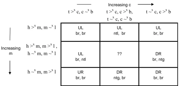
Given this sequence of evaluations and responses, outcomes of the generalized stag-hunt discussed earlier will vary as the value of the intermediate payoffs, m and c, increase in value as shown in Table 9.
Table 9 t >x c, c ~x b t >x c, c >x b, t ~x c, c ~x b t ~x c, c >x b h >x m, m ~x l UL UL UL br, br ntl, br br, br Increasing m h >x m, m >x l , h ~x m, m ~x l UL ?? DR br, ntl br, ntg h ~x m, m >x l UR DR DR br, br ntg, br br, br Increasing c
Beginning in the upper left hand cell, Player 2, perceiving Player 1’s high payoff as dissimilar to the middle one and the middle as similar to the worst, will predict that Player 1 will choose U. In this case, Player 2 will best respond by choosing L
independent of what he perceives regarding his own payoffs (i.e., P2 will best respond with L for all cells in the top row of Table 9.) Player 1, viewing Player 2’s top prize as dissimilar to the center one and the center as similar to the bottom, will expect Player 2 to choose L and best responds with U, once again independent of the similarities or dissimilarities among his own payoffs (i.e., in each cell in the first column of table 9.) Predictions for the remaining cells are obtained in the same fashion.
The predictions that follow if agents consider the similarities and
dissimilarities of the other player’s payoffs first, summarized in table 9, are identical to those that follow if players consider their own payoffs first, summarized in Table 4, with two critical exceptions – the predicted responses in the southwest and northeast cells in the tables. These cases correspond to situations in which the configurations of similarities and dissimilarities suggest that one player has “nothing to gain” by
choosing the strategy offering the best possible outcome and the other has “nothing to lose” by doing so as was the case in Game III-I discussed earlier and reproduced below. L R Player 1 U 8.00, 8.00 2.00, 2.10 D 7,90, 2.00 7,90, 2.10 III-I Player 2
Recall that in this game, the intermediate value payoff, m, to Player 1 is made large, while the intermediate payoff, c, is made small. The first manipulation
promotes the perception of h ~x m and m>x l in which case there appears to be “nothing to gain” by choosing strategy D offering the highest payoff. The second manipulation promotes the perception of t >x c but c ~x b in which case there is “nothing to lose” by choosing the highest payoff option L. Given these predictions we expected the non-equilibrium outcome DL to predominate in the game – and it did.
But now think what happens when the opponent’s payoffs are considered first. In this case, Player 1 will conclude that Player 2 is going to choose L and best
responds by choosing U. Player 2 will conclude that Player 1 is going to choose D and best respond with R. Together, these decisions produce the mirror image non-equilibrium outcome UR.
This analysis suggests that, if subjects are really employing similarity
judgments to make their strategy choices and if we can frame the game in such a way as to prompt subjects to consider the other player’s payoffs first, we will reverse their strategy choices and obtain the alternative non-equilibrium outcome.
To test this prediction, subjects were presented with the following game:
If Other chooses L and you choose U You receive 7.20 and Other receives 7.20
D 7.10 1.20
If Other chooses R and you choose U You receive 1.20 and Other receives 1.30
D 7.10 1.30
Given the payoffs Other faces, what choice do you predict he or she will make? L_____ or R_____
Please indicate which choice you would like to make. U_____ or D_____
This question, denoted III-I*, was always the last game posed to subjects. The game itself is derived by subtracting .80 from each of the payoffs in Game III-I. It also differs from Game III-I in that here subjects were explicitly asked to first predict what strategy the other player is going to choose and then what strategy they wish to
choose – this is the re-framing intended to produce the strategy reversals. As indicated in Table 10 neither difference has any influence on the predictions of the equilibria selection criteria discussed early nor do they change the optimal mixed strategies for the game – all predictions are identical to those for Game III-I. Moreover, without some sort of ancillary theory of how the noise in introspection varies with the way the problem is posed, no change in behavior would be predicted by a quantal response model.
L R L R Player 1 U 8.00, 8.00 2.00, 2.10 Player 1 U 7,20, 7,20 1,20, 1,20 D 7.90, 2.00 7.90, 2.10 D 7,10, 1,20 7,10, 1,30 m=c= Payoff Dominant Eq. UL UL Security-minded eq. DR DR Risk dominant
eq. Neither Neither
Mixed strategy eq. DL p(U)=.0167, p(L)=.9833 DL p(U)=.0167, p(L)=.9833 ntg/ntl outcome DL UR L R L R Player 1 U 41% 4% 17 (45%) Player 1 U 54% 25% 30 (79%) D 51% 4% 21 (55%) D 5% 3% 8 (21%) 35 (92%) 3 (8%) 26 (68%) 12 (32%) U9 D9 L9 R9 U4 36% 9% 17 (45%) L4 63% 29% 35 (92%) D4 43% 12% 21 (55%) D9 5% 3% 3 (8%) 30 (79%) 8 (21%) 26 (68%) 12 (32%) III-I III-I* Player 2 Player 2 m=7,9, c=2,1 m=7,1, c=1,2
Responses and Implied Outcome Frequencies
III-I III-I*
Player 2 Player 2
Player 2 Player 2
III-I III-I*
Results are shown in Table 10. Consistent with the predictions that follow if subjects choose strategies based on similarity judgments and if the framing manipulation employed succeeded, the proportion of Player 1s choosing U in III-I* (79%) is significantly larger than the percentage of Player 1s choosing U in III-I (45%) (χ2
1df
=6.8571, p=.0088) and the proportion of Player 2s choosing R in III-I* (32%) is significantly larger than the percentage of Player 2s choosing R in III-I (8%) (χ2
1df =
To close it is worth noting that the data on play in games III-I and III-I*, though largely consistent with the predictions following from the hypothesis that people base their choices on similarity judgments, also suggest that the framing manipulation employed in game III-I* was not entirely successful. In particular, note that while the non-equilibrium outcome DL expected to predominate in game III-I does predominate (51%) the predominant pattern in III-I* is UL (54%) and not UR (25%) as expected. The responses for Player 1s and Player 2s conditional on what they expected the other player to do, shown in Table 11, suggest why this is the case. Table 11 L R U D Player 1s U 30 (79%) 0 Player 2s L 16 (42%) 10 (26%) Choice D 8 (21%) 0 Choice R 1 (3%) 11 (29%) 38 (100%) 17 (45%) 21 (55%) Prediction Regarding Player 2's Choice Prediction Regarding Player 1's Choice
Specifically, notice that all Player 1s predict Player 2 will choose L (the “nothing to lose” response) and 79% best respond to this prediction by choosing U. For Player 2s, in contrast, only a slight majority predict Player 1 will choose D ( the “nothing to gain” response) and of these only a slight majority, 11 versus 10, best respond by choosing R. The rest of those that predict Player 1 would choose D apparently decide they have “nothing to lose” in any case and pick L. The remaining large minority of Player 2s (45%) predicted Player 1 would choose U and virtually all best responded given that prediction. These results again suggest that the comparison processes players employ may be more complex than modeled here and also raise the possibility that subjects find that situations in which there is “nothing to lose” provide
more compelling reasons to choose one strategy over another than situations in which there is “nothing to gain.”
Discussion
Game theory provides an elegant, logically compelling, description of what the outcomes of strategic interactions among players who are fully rational,
computationally unconstrained and infinitely discerning with regard to payoffs will be. These normative virtues notwithstanding, experiments have shown the theory is limited as a descriptive model of strategic interaction. This problem has not gone unnoticed – indeed, John Nash, whose name graces the fundamental concept in game theory, is said to have abandoned the enterprise upon realizing that behavior departed systematically from what became known as Nash equilibrium. Those less fatalistic, or maybe less realistic, have addressed the descriptive limitations of the theory differently – adding auxiliary assumptions of a rational ilk upon a theory already laden with a very strong dose of rationality. In this paper, I have taken a rather different tack based on three observations. The first is that it seems plausible that if people misbehave vis-a-vis rationality in choices, they will probably do so in more complex, strategic settings. The second is that most of the misbehavior in choice seems to stem from a tendency not to discriminate between magnitudes – payoffs, probabilities, time periods – that are in, at least a relative sense, close in value. The third is that what seems to drive the misbehavior resulting from this failure to
discriminate is the perception that there is either “nothing to gain” or “nothing to lose” by following one course of action over another.
We have examined the consequences of such reasoning in the context of coordination games and games of pure conflict. Experimental results, with one
exception, bear out the hypotheses that follow from the assumption that players’ base their strategic choices on the “nothing to gain/nothing to lose” effect. In the context of coordination games, we obtain an explanation for why people sometimes play strategies corresponding to payoff dominance (because there is “nothing to lose” by doing so) and sometimes play strategies corresponding to security-mindedness (because there is “nothing to gain” by doing otherwise). As we have seen, these effects can conspire under the right circumstances to produce non-equilibrium outcomes. 14
In the context of games of conflict, we have seen that the same effects can produce systematic game outcomes even though these games contain no pure strategy equilibria. Moreover, these systematic effects cannot be attributed to subjects playing mixed strategies.15
Taken together the approach to understanding play in games presented here and the evidence testing its predictions raise an interesting possibility -- that, though individually irrational, “nothing to gain/nothing to lose” reasoning may be adaptive, if not optimal, from a social standpoint to the extent that it provides people with a theory of focality – and one that under many circumstances produces what, to the layman if not the economist, are sensible outcomes. In standard game theory, coordination games are problematic precisely because there isn’t any guidance as to which of the multiple equilibria people should aim for. With apologies in advance of exploiting a sort of creeping cardinality, if we add a little inability or unwillingness to discriminate between payoffs in coordination games, we gravitate toward payoff dominant
equilibrium when the payoffs involved in one cell are dramatically superior to those
14 Although, interestingly, the outcome is an equilibrium in a transformed game in which the similar payoffs are equated.
in the other cells in the game as in Game I-I in Table 5. Likewise, we gravitate toward the security-minded equilibrium when the only real problem in the game is avoiding the worst possible payoffs contained in the non-equilibrium game outcomes (as in Game III-III in Table 5.) That a combination of “nothing to gain” and “nothing to lose” effects can conspire to produce an outcome dominated by both equilibria as was the case with DL in Game III-I may be unfortunate but these effects
simultaneously insure that the socially disastrous outcome UR will not occur. In a related vein, in conflict situations, game theory’s predictions are pretty grim. However, add a little unwillingness or inability to discriminate, and we end up with at least a subset of possible games where both players receive an outcome which is jointly superior to any other available (compare the predicted outcome in Game VI-I with the other cells in that game) and superior to anything that could be achieved through randomization.
I do not know at this point whether these types of conclusions regarding the potential benefits of “nothing to gain/nothing to lose” type reasoning are robust. What does seem beyond question at this point is that the role of such reasoning in games – still other types of games, more complex games, games with repetition, games with communication, etc. - is critical if we are to understand real strategic interactions.
Bibliography
Azipurua, J., I. Nieto, and J. Uriate, “Similarity and Preferences in the Space of Simple Lotteries,” Journal of Risk and Uncertainty, 1993, 6, 289-297.
Beard, T. and R. Beil. “Do People Rely on the Self-Interested Maximization of Others? An Experimental Test.” Management Science. 1994, 40, 252-262.
Buschena, D., and D. Zelberman, “Performance of the Similarity Hypothesis Relative to Existing Models of Risky Choice,” Journal of Risk and Uncertainty, 1995, 11, 233-262.
Camerer, C. Behavioral Game Theory: Experiments on Strategic Interaction, Princeton, 2003.
Camerer, C.F., Ho, T-H, Chong, J-K. "A Cognitive Hierarchy Model of One-Shot Games," Quarterly Journal of Economics, August 2004, 119(3), 861-898.
Costa-Gomes, M., V. Crawford, and B. Broseta. "Cognition and Behavior in Normal-Form Games: An Experimental Study," Econometrica, September, 2001. Vl. 69(5), 1193-1235.
Goerree, J. and C. Holt. “Ten Little Treasures of Game Theory and Ten Intuitive Contradictions.” American Economic Review. 2001. Vl. 91(5), pp 1402-1422. Goerree, J. and C. Holt. “A Model of Noisy Introspection.” Games and Economic Behavior, 2004, 46(2), 365-382.
Goerree, J., C. Holt and T. Palfrey. “Regular Quantal Response Equilibrium.” Experimental Economics, 2005, 8, 347-367.
Gonzalez-Vallejo, C. “Making Trade-Offs: A Probabilistic and Context-Sensitive Model of Choice Behavior. Psychological Review. 2002, Vl. 109. pp 137-155. Haruvy, E. and D. Stahl. “Deductive versus Inductive Equilibrium Selection - experimental results.” Journal of Economic Behavior and Organization. 2004, 53, 319-331.
Keser, C. and B. Vogt. “Why do experimental subjects choose an equilibrium which is neither risk nor payoff dominant?” Working paper, 2000.
http://www.cirano.qc.ca/pdf/publication/2000s-34.pdf
Leland, J. "Individual Choice Under Uncertainty: Finite Discriminatory Ability and Systematic Deviations from 'Strict' Rationality". Doctoral Dissertation, University of California, Los Angeles, 1986.
Leland, J. "Generalized Similarity Judgments: An Alternative Explanation for Choice Anomalies." Journal of Risk and Uncertainty, 9, 1994, 151-172.
Leland, J. “Similarity Judgments in Choice Under Uncertainty: A Reinterpretation of Regret Theory.” Management Science, 44(5), 1998, 1-14.
Leland, J. “Similarity, Uncertainty and Time – Tversky (1969) Revisited,” IBM Research Report RC22120 (99107) July 18, 2001.
http://www.research.ibm.com/iac/papers/RC22120.pdf
Leland, J. “Similarity Judgments and Anomalies in Intertemporal Choice.” Economic Inquiry Vol. 40, No. 4, October 2002, 574-581.
Loomes, G. “The Improbability of a General, Rational and Descriptively Adequate Theory of Decision Under Risk.” 2006.
McKelvey, R.and T. Palfrey. “Quantal Response Equilibria for Normal Form Games." Games and Economic Behavior. 1995, 10, 6-38.
Markman, A., and D. Medin, “Similarity and alignment in choice,” Organizational Behavior and Human Decision Processes, 1995, 63, 117-130.
Medin, D., R. Goldstone, and A. Markman, “Comparison and Choice: Relations between similarity processes and decision processes,” Psychonomic Bulletin & Review, 1995, 2(1), 1-19.
Mellers, B., and K. Biagini, “Similarity and Choice,” Psychological Review, 1994, 101, 505-518.
Montgomery, H., “Decision Rules and the search for dominance structure: Towards a Process Model of Decision Making,” in Analyzing and Aiding Decision Processes, eds. P.
Humphreys et al, Amsterdam, the Netherlands, North Holland, 1983, 342-369.
Palfrey, T. “McKelvey and Quantal Response Equilibrium.” Forthcoming in A Positive Change in Political Science: The Legacy of Richard D. McKelvey’s Most Influential Writing. Edited by J. Alt, J. Aldrich and A. Luipia. Univerisity of Michigan Press. 2005.
Rubinstein, A. "Similarity and Decision-making Under Risk (Is There a Utility Theory Resolution to the Allais Paradox?)." Journal of Economic Theory, 46, 1988, 145-153.
Rubinstein, A. “Economics and Psychology"? The Case of Hyperbolic Discounting, International Economic Review 44, 2003, 1207-1216.
Rydval, O. and A. Ortmann. “Loss Avoidance as a Selection Principle: Evidence from Simple Stag Hunt Games.” Economics Letters, Volume 88, Issue 1, July 2005, Pages 101-107.
Tversky, A., "Intransitivity of Preferences," Psychological Review, 1969, 76(1), 31-48.
Vogt, B., and W. Albers. “Equilibrium selection in 2x2 bimatrix games with preplay communication. 1997, IMW Working Paper 267. University of Bielefeld.
D.J. Zizzo Preliminary Experimental Results on the Similarity Function in 2x2 and 3x3 Games." Working Paper, 2002