INTRODUCTIVE REMARKS ON CAUSAL INFERENCE S.A. Romio, R. Bellocco, G. Corrao
1. INTRODUCTION
Both estimation and interpretation of causal effects in epidemiological studies aimed to assess the effect of well defined risk factors on the incidence and prog-nosis of cancer and other chronic conditions represent a key step in the under-standing of complex disease mechanism. Randomized clinical trials, under some desirable conditions, represent the ideal type of study (gold standard) where causal effects can be estimated. Indeed, in this type of studies, association is cau-sation (Hernàn and Robins, 2006). Unfortunately, in observational studies, such as cohort or case-control, the problem of causation is indeed not straightforward. Confounding is one of the possible biases that can arise in the estimation of parameters in such studies. This particular type of bias, well known by epidemi-ologists, has generated recently a lot of debate as there have been situations where the standard definition are been proved to be wrong, requiring then a wider formalization. Confounding is strongly and closely related to the study of causal exposure-outcome relationship.
One of the approaches developed and supported in the last decade to estimate the causal effect is based on the concept of counterfactuals. In this setting, in-stead of dividing the population and comparing subgroups of exposed and unex-posed individuals, the whole population is considered first under exposure and in a second time under not exposure. Unfortunately, almost no study designs are available to rewind time and so to assess the same individual under different con-ditions.
Under the assumption of exchangeability between exposed and unexposed subjects, usually a valid assumption in randomized or conditional randomized clinical studies, it is possible to create “pseudo-population”, where indeed all pos-sible form of contrasts (differences or ratios) can have a causal interpretation.
This leads to a natural measure of causation based on marginal probabilities rather than on conditional probabilities. The estimator obtained under this frame-work, based on the Inverse Probability Weighted Treatment method, is analogous to the well known Horvitz-Thompson estimator for finite populations (Hernàn and Robins, 2006; Horvitz and Thompson, 1952).
A basically equivalent approach relies on standardization. These two ap-proaches requires the same hypotheses to be able to give estimates of causal effects. Moreover, these estimations are identical in simple situations (time invariant exposures) (Hernàn and Robins, 2006).
The present paper is organized as follows. Section 2 provides a comparison of the concepts of association and causality. Section 3 presents the concept of con-founding under a causal framework and in section 4 the definition of causality in epidemiology is formally stated. Section 5 through a simple example, shows two of the main methods used for the estimation of the causal effect. Finally, in sec-tion 6 we make some theoretical and practical conclusions related to the estima-tion of causal effect in observaestima-tional studies.
2. ASSOCIATION AND CAUSALITY
The aim of most epidemiological studies is to assess the association between a risk factor and an outcome. But, explicitly or implicitly, the interpretation of
association is often confused with causality even though the two concepts are
differ-ent. In general, the causal structures related to the association relationship be-tween an exposure (E) and an outcome (D) are the following (Greenland and Pearl, 2006):
- E can cause D (true causal effect), - D can cause E (reverse causation),
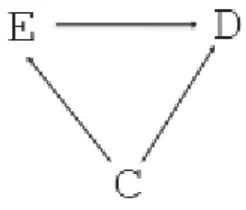
- E and D can share a common cause (the confounder) (Figure 1),
- E and D share a common effect (the collider) (e.g. Berksonian bias) (Figure 2).
Figure 1 – Confounding bias: E is high cholesterol level, C is stress (Steptoe and Brydon, 2005), D is stroke.
Figure 2 – Berksonian bias: E is high cholesterol level, D is stroke, C is the collider (an index meas-uring quality of life).
The misunderstanding of the definition of association and causation has lead to a revision of the two concepts. A very simple way to well characterize them is assuming that causation has a defined direction, that is a non-symmetric relation-ship, while association is described by an undirected relationship (that is symmet-ric) (Greenland, 2004).
Of course, the concept of causality concerns not only medical and biological sciences, but many other disciplines, such as sociology, economics, demography, and it has been well studied in philosophy. Indeed, in the XVIIIth century, Hume tried to cope with this issue and defined a cause as a necessary condition for the consequence. To be specific, he stated: “we may define a cause to be an object, followed
by another, and where all the objects similar to the first are followed by objects similar to the sec-ond. Or in other words where, if the first object had not been, the second never had existed”
(Hume, 1748). Related to this definition the concept of counterfactual was pro-posed in philosophy during the last century. This concept, that means contrary to the fact, was recently proposed by some influential statisticians, biostatisticians, and computer scientist (Rubin, Greenland, Robins and Pearl) to develop novel statistical models which allows for the different estimation of the causal effect of one or more factors on the outcome of interest.
This causal effect can be measured using the same measures that we use for the association but using a different kind of populations. To fix ideas, it is possi-ble to compute rate and risk differences (RD), rate and risk ratios (RR) or to es-timate the causal effect. But, while the association measure compares what has happened in two different sub-groups of the population being studied, that is un-der di erent conditions that are both observable (for instance subjects with high cholesterol level and subjects with low cholesterol level), the causal e ect measure compares the outcome in a unique population under different conditions, but only one of them is observable (what happens if everybody would have had high cholesterol level compared to the situation where nobody would have had that high level). (Hernàn, 2004).
3. CONFOUNDING AND CAUSALITY
One of the problems that often arise in epidemiological studies is confound-ing. Probably, confounding is the most used concept in the literature even if the most difficult to define, particularly when there might be a time dependency. Dif-ferent definitions have been given for confounding. The standard definition of confounding is the one shown in figure 1 where the confounder C is associated to the exposure E and to the outcome D given E but it is not in the pathway from E to D.
A well known similar definition is the one based on the concept of collapsabil-ity, where C is a confounder if the conditional (within level of C) association be-tween E and D is different than the unconditional (crude) association measure (e.g., if adjusted risk ratio changes by more than 10% compared with unadjusted odds ratio). As clearly proven in many papers (Greenland et al., 1999; Miettinen
and Cook, 1981) collapsability is a necessary condition for confounding but not sufficient. The issue with this definition is that differences between conditional and unconditional association measures are expected with non-collapsible meas-ures (Miettinen and Cook, 1981) even in the absence of common causes (e.g., in ideal randomized experiments).
An alternative to the usual definitions of confounding is the causal definition: we say that confounding is present when the considered association measure is not equal to the causal measure e.g. when the causal relative risk is not equal to the (association) relative risk (Hernàn, 2004).
Therefore exposed and not exposed are not comparable, because of presence of a common cause. In this definition, it becomes clear the distinction between the concept of confounding (presence of a common cause) and the confounder, any variable that can be used to eliminate confounding.
Under this point of view, the issue becomes how to calculate the causal meas-ures. In the next two sections we will be showing the assumptions needed for the equivalence between causal and association measures and an example will be pro-vided.
4. CAUSALITY IN EPIDEMIOLOGY
We present the concepts of association and causation under a formal point of view. The association between a factor E (e.g. cholesterol level) and an outcome
D (e.g. stroke) is expressed by
P[D=1|E=1] P[D=1|E=0] (1)
Indeed, equation (1) represents the fact that the probability of the outcome D is different in the two different sub-populations subjects with E=0 and subjects with E=1, which is what we have highlighted in the previous section. In the ex-ample, and for seek of semplify, we consider only two categories for the exposure
E: high level (E=1) and low level (E=0). Therefore, the two probabilities are the
probability of stroke in the population of subjects with high cholesterol level and the probability of stroke in the population of subjects with low cholesterol level. The comparison beween the two probabilities in equation (1) can be performed in the standard way, i.e using risk differences (RD), risk ratios (RR) or odds ratio (OR).
However, to evaluate the causal effect of exposure E on outcome D it is nec-essary to consider the same population but in two different situations. This means that we have to consider the population under study when every subject has high cholestrol level and the population under study when every subject has low cho-lestrol level. For each population, we define the counterfactual outcomes De=1
and De=0 i.e. the new random variables that represent the outcome D had every
subject been exposed to E (e.g. had had high cholesterol level) and the outcome
Of course, for each subject, only one counterfactual outcome can be observed, the other is missing. Using this new counterfactual random variables, the expo-sure has a causal effect at subject level if and only if, for each subject
De=1 De=0 (2)
To assess this causal effect we should test the sharp causal null hipothesis i.e.
De=1 = De=0 (3)
but, because of the missing information, it is not possible to test this hypothesis. Instead of this, we can test the population level null hypothesis
P[De=1=1]= P[De=0=1] (4)
This hypothesis is a particular case, when the outcome is dicotomous, of the more general definition (Hernàn, 2004):
Definition 1: We say that exposure A has a mean causal effect on the outcome Y in
the population if and only if
E[De] E[De’] (5)
for each pair (e, e’) where ee’.
Analogously to the association measures, we can define the causal measures us-ing P[De=1=1] and P[De=0=1]. These measures use marginal probabilities instead
of conditional probabilities, as association measures.
To be able to estimate these measures, we need a further hypothesis, i.e. the exchangeability: this hypothesis, that is implied by randomization in clinical trials, should be considered carefully in observational studies. Under this hypothesis, we have:
P[De=1|E=1] = P[De=1|E=0] = P[De=1] (6)
Because of
P[De=1|E=e] = P[D=1|E=e] (7)
combining (6) and (7) we obtain
P[De=1] = P[De=1|E=e] = P[D=1|E=e]
P[De=1] = P[D=1|E=e] (8)
Therefore, exchangeability implies that association is causation (Hernàn, 2004). In the setting of observational studies, this condition often does not hold be-cause of the presence of a predictive factor that can influence the exposure of in-terest i.e. a confounder. In the previous example we can consider as a predictor factor C the typology of work as an indicator of the stress. The exchangeability condition becames conditional exchangeability (Hernàn and Robins, 2006)
P[De=1|E=1; C=c] = P[De=1|E=0; C=c]
= P [De=1|C=l] (9)
i.e. De E|C e. However, to calculate the causal effect of the exposure, the
confounder should be measured.
Together with the previous hypothesis of conditional exchangeability, there are other two assumptions: the consistency and positivity. The former one can be de-scribed as follows: De=D if E=e is the actual level of the expoure and regards the
fact that the counterfactual outcome is well defined. The second one P[E=e|C=c] > 0 if P[C = c] 0 ensures the existence of the standardized risk because it ap-pears in the denominator of the terms of this risk.
There are several approaches to calculate the causal effect in observational studies. We will focus on two of them: Standardization (S) and Inverse Probabil-ity of Treatment Weighting (IPTW). The two methods are equivalent and based on the same hypothesis. However, the main difference between them is the fact that they use different modelling assumptions to calculate the probabilities that appear in the relative risk (i.e. P[De=1|E=e; C=c] and P[C=c]). Of course, in the
most simple dicotomous situation, the two methods produce equal results (Hernàan and Robins, 2006).
In the next section we present the two methods for the calculation of the causal effect through a simple example.
5. EXAMPLE
In this example we will show how to calculate the causal relative risk using both the standardization and the inverse probability treatment weight approaches. The fictitious data are showed in table 1. As in the previous section, D represents the dichotomous outcome stroke (Yes/No), E represents the exposure of interest cholesterol level (High/Low) and C the potential measured confounder stress (Yes/No). Table 2 shows how each method calculates the RR.
TABLE 1
Fictitious data
C=0 C=1
E=0 E=1 E=0 E=1
D=1 2 2 3 6
D=0 2 1 2 2
4 3 5 8
TABLE 2
Methods to calculate the RR
Standardization (S) IPTW
Pr[D=1|E=1] Pr[D=1|E=0]
Pr[De=1=1]
To apply the IPTW method we need the frequencies of the counterfactual outcomes i.e. the probabilities of the outcome in the new population, the pseudo-population (Hernàn and Robins, 2006). In this pseudo-population the probabilities of the outcome are proportional to the original ones: specifically, the probabilities of the outcome D for each category of the confounder are cal-culated as the original probabilities times the inverse of the corresponding con-ditional probability P(E = e|C=c). This is due to the fact that the pseudo-population should reflect what happen in the original pseudo-population first consider-ing the hypothesis that every subject had been exposed and then considerconsider-ing the hypothesis that every subject had been not exposed. Tables 3 and 4 shows the frequencies of the populations had every subject remained unexposed and exposed respectively.
TABLE 3
All subjects unexposed
C=0 C=1
D=1 7/2 39/5 D=0 7/2 26/5
7 13
TABLE 4
All subjects exposed
C=0 C=1
D=1 14/3 39/4 D=0 7/13 13/4
7 13
Therefore, the inverse of these probabilities are the weights needed to adjust the original frequencies of the outcome to obtain the new frequencies in the pseudo- population. In our example the weights are showed in table 5.
TABLE 5 Weights IPTW C E P(E=e|C=c) W 0 0 4/7 7/4 0 1 3/7 7/3 1 0 5/13 13/5 1 1 8/13 13/8
Table 6 shows the frequencies for the pseudo-population. TABLE 6
Pseudo-population frequencies
C=0 C=1
E=0 E=1 E=0 E=1
D=1 7/2 14/3 39/5 39/4
D=0 7/2 7/13 26/5 13/4
As it is easy to see, the number of the subjects in the pseudo-population is twice the number of the subjects in the original one (i.e. 40 instead of 20). Using the previous tables, the estimation of the RR is straightforward.
For the (S) method we have:
Pr[ 1| ; 1]Pr[ ] Pr[ 1| ; 0]Pr[ ] c c D C c E C c RR D C c E C c
2/3(7/20) 3/4(13/20) 2/4(7/20) 3/5(13/20) 14/3 39/4 7/2 39/5 (10)while for the (IPTW) method, the estimation of the RR becames:
1 0 Pr[ 1] 14/3 39/4 Pr[ 1] 7/2 39/5 e causal e D RR D (11)
that is the same result obtained with the (S) method. Of course these calculations rely on the hypothesis of conditional exangeability discussed in the previous section. 6. CONCLUSIONS
In this paper we have reviewed the concept of causality and some important issues related to it. We have focused on the particular problem of the estimation of the causal effect in the epidemiological context. We have considered only two of the available methods to estimate the causal effect. Through a simple example we showed that the two methods (S) and (IPTW) took into account lead to the same value of the measure considered (i.e. the RR). Some remarks are worthy of consideration.
Firstly, the two methods have the common assumption of conditional ex-changeability for exposed and unexposed.
Secondly, the two methods require the non-existence of unmeasured con-founders (Hernàn and Robins, 2006) in order to identify the causal effect. Unfor-tunately, this hypothesis cannot be always tested based on the available data, sce-nario very similar to the missingness at random in the context of missing data problem.
Thirdly, even if the two methods are equivalent in the most simple cases (as the one showed in this paper) they can produce different estimations, for exam-ple, if a time dependent variable is present (Hernàn and Robins, 2006). In this situations, it is diffcult to stratify, and the estimation of the terms in the RR ex-pression should be done superimposing a statistical model. The choice of the model and the different assumptions considered by them can produce differences in the results obtained from the two methods.
Finally, a further important remark is the different nature of the two ap-proaches: standardization is based on conditional probabilities while inverse probability of treatment weighting use marginal probabilities.
The advantage of these methods, compared to classical methods, based on stratification, such as Mantel-Haenzel or logistic regression, is that under the as-sumption of non unmeasured confounding, the quantity being estimated can be interpreted always in terms of causal effect. Moreover, in more complex mecha-nisms, standard regression methods will not be able to take properly into account the confounders or the colliders and the analysis produced will be biased.
7. ACKNOWLEDGMENT
We like to thank our Computer Assistant, Riccardo Giani from the Depart-ment of Statistics, University of Milano-Bicocca for his expertise in both hard-ware and softhard-ware management.
Rino Bellocco e Giovanni Corrao received grants from the Italian “Fondo d’Ateneo per la ricerca”.
Department of Medical Informatics Erasmus Me SILVANA A. ROMIO
Department of Statistics University of Milano-Bicocca
Department of Medical Epidemiology and Biostatistics RINO BELLOCCO Karolinska Institutet
Department of Statistics GIOVANNI CORRAO
University of Milano-Bicocca
REFERENCES
S. GREENLAND,(2004),Applied Bayesian Modeling and Causal Inference form Incomplete-Data
Per-spectives, Wiley & Sons.
S. GREENLAND, J. PEARL,(2006),Causal Diagrams, Computer Science Department. University
of California, Technical Report R-332.
S. GREENLAND, J.M. ROBINS, J. PEARL, (1999), Confounding and Collapsability in Causal Inference,
“Statistical Science”, 14:29-46.
M.A. HERNÀN,(2004), A definition of causal effect for epidemiological research, “Journal of
Epidemi-ology and Community Health”, 58:265-271.
M.A. HERNÀN, J.M. ROBINS, (2006), Estimating causal effect for epidemiological data, “Journal of
Epidemiology and Community Health”, 60:578-586.
D.G. HORVITZ, D.J. THOMPSON,(1952), A generalization of sampling without replacement from a finite
population, “Journal of the American Statistical Association”, 647:663-685.
D. HUME, (1748), An Enquiry Concerning Human Understanding, section VII, part II.
O. MIETTINEN, E.F. COOK, (1981), Confounding: Essence and Detection, “American Journal of
Epidemiology”, 114:593-603.
A. STEPTOE, L. BRYDON, (2005), Association between acute lipid stress responses and fasting lipid levels
SUMMARY
Introductive remarks on causal inference
One of the more challenging issues in epidemiological research is being able to provide an unbiased estimate of the causal exposure-disease effect, to assess the possible etiologi-cal mechanisms and the implication for public health. A major source of bias is con-founding, which can spuriously create or mask the causal relationship. In the last ten years, methodological research has been developed to better de_ne the concept of causa-tion in epidemiology and some important achievements have resulted in new statistical models. In this review, we aim to show how a technique the well known by statisticians, i.e. standardization, can be seen as a method to estimate causal e_ects, equivalent under certain conditions to the inverse probability treatment weight procedure.