Study of cosmic nuclei fluxes with AMS-02: implication for dark matter search

Alma Mater Studiorum

· Università di Bologna

Scuola di Scienze

Corso di Laurea Magistrale in Fisica

Study of Cosmic Nuclei fluxes with AMS-02:

implication for Dark Matter Search

Relatore:

Prof. Andrea Contin

Correlatore:

Dott. Nicolò Masi

Presentata da:

Nicoletta Belloli

Sessione II

Abstract

L’Alpha Magnetic Spectrometer (AMS-02) é un rivelatore per raggi cosmici (CR) pro-gettato e costruito da una collaborazione internazionale di 56 istituti e 16 paesi ed installato il 19 Maggio del 2011 sulla Stazione Spaziale Internazionale (ISS).

Orbitando intorno alla Terra, AMS-02 sará in grado di studiare con un livello di ac-curatezza mai raggiunto prima la composizione dei raggi cosmici, esplorando nuove frontiere nella fisica delle particelle, ricercando antimateria primordiale ed evidenze indirette di materia oscura.

Durante il mio lavoro di tesi, ho utilizzato il software GALPROP per studiare la propagazione dei CR nella nostra Galassia attraverso il mezzo interstellare (ISM), cer-cando di individuare un set di parametri in grado di fornire un buon accordo con i dati preliminari di AMS-02. In particolare, mi sono dedicata all’analisi del processo di propagazione di nuclei, studiando i loro flussi e i relativi rapporti .

Il set di propagazione ottenuto dall’analisi é stato poi utilizzato per studiare ipotetici flussi da materia oscura e le possibili implicazioni per la ricerca indiretta attraverso AMS-02.

Contents

1 Introduction 3

2 Propagation of Cosmic Rays in the Galaxy 5

2.1 Origin of Cosmic Rays . . . 7

2.2 Spectroscopy: Physics of Cosmic Nuclei . . . 10

2.3 Acceleration and Propagation Mechanism . . . 12

2.3.1 Diffusion Halo Model . . . 18

2.3.2 Weighted Slab Model . . . 24

2.3.3 Leaky Box Model . . . 25

2.4 Cosmic Rays at the Top of the Atmosphere . . . 26

3 Dark Matter Physics 30 3.1 ΛCDM Model . . . 31

3.1.1 Friedmann Equations . . . 32

3.1.2 Universe Classification . . . 33

3.1.3 Dark Matter Production in the ΛCDM Model . . . 35

3.2 Dark Matter Candidates after the Higgs Boson Discovery . . . 38

3.3 Dark Matter Search in Space with AMS-02 . . . 54

3.3.1 Experimental Results from PAMELA and Fermi . . . 54

3.3.2 Indirect Dark Matter Search . . . 55

4 AMS-02 62 4.1 The Experiment: Goals and Measurements . . . 63

4.2 Transition Radiation Detector (TRD) . . . 64

4.3 Time of Flight (TOF) . . . 65

4.3.1 How it works . . . 66

4.3.2 Electronics . . . 70

4.4 The Magnet . . . 72

4.6 Ring Imaging Cherenkov (RICH) . . . 74

4.7 ECAL . . . 77

4.8 ACC, TAS and Star Tracker . . . 79

5 The GALPROP Software 82 5.1 GALPROP Model . . . 82

5.2 Galaxy Structure . . . 83

5.2.1 Galactic Source Distribution . . . 85

5.2.2 Interstellar Gas Distribution . . . 85

5.3 Galactic Magnetic Field . . . 87

5.4 Isotopic Abundances . . . 87

5.5 Propagation Equation . . . 88

5.6 Iniection Spectra and Diffusion Coefficients . . . 90

5.7 Modulation in the Heliosphere . . . 94

5.8 Dark Matter in Galprop . . . 95

6 Analysis of Nuclei Fluxes: a Comparison between Data and Theory 97 6.1 Analysis Strategy . . . 97

6.2 Choice of the Propagation Set with Galprop . . . 101

6.2.1 Galaxy Geometry and Propagation Mechanisms . . . 101

6.2.2 Spectral Indices . . . 115

6.2.3 Primary Abundances at Source . . . 121

6.2.4 Nuclear Cross Sections . . . 125

6.2.5 Solar Modulation and overall uncertainty . . . 128

6.3 Galprop Results . . . 133

6.3.1 Chi-Squared Test . . . 134

6.4 Dark Matter Physics with GALPROP and PPPC4DMID . . . 138

6.4.1 The PPPC4DMID Software . . . 143

7 Conclusion 154

Chapter 1

Introduction

I carried out my thesis project with the Bologna INFN research group, responsible for the Time of Flight (TOF), for the AMS-02 experiment (Alpha Magnetic Spectrome-ter).

AMS-02 is a space born detector for cosmic rays (CR), built to work as an external module of the International Space Station (ISS). It was installed on 19 May 2011 aboard of the ISS, during the flight of the mission STS-134 of the Shuttle Endeavour. The experiment is an improved version of a precedent experiment, AMS-01, which flew on board of the Shuttle Discovery on June 1998.

The main goals of the experiment are: the precision measurement of the CR fluxes and composition, the detection of possible dark matter signals and the discovery of antimatter.

During my thesis I focused on the study of CR propagation through the Interstellar Medium (ISM) up to the top of the atmosphere. The main task of my work was to identify a propagation set able to give the best fit of the AMS preliminary data and able to give some hints about the DM production, maintaining a good agreement with the avaible data.

After a brief introduction on my work, in the second chapter I will give a general description of cosmic rays propagation in the galaxy.

In the third chapter I will introduce the Dark Matter physics, discussing on the main candidates and how we can look for DM with AMS-02.

The fourth chapter is devoted to the structure of the AMS-02, highlighting the impor-tance of each detector that composes the experiment.

In the fifth chapter I will treat in detail the software I worked with for the study of CR propagation, GALPROP, describing the tuning parameters I used for my study. In the sixth chapter I will explain the main procedure of analysis I used for the

com-parison between data and theory for the study of nuclear fluxes and ratios, showing the fallout one can obtain on dark matter physics.

Here it was chosen to show only preliminary data for nuclei: these data are still under study by the collaboration and not yet published in an official paper.

Chapter 2

Propagation of Cosmic Rays in the

Galaxy

In August 1912, Austrian physicist Victor Hess made a historic balloon flight that opened a new window on matter in the universe. As he ascended to 5300 meters, he measured the rate of ionization in the atmosphere and found that it increased to some three times that at sea level. He concluded that penetrating radiation was entering the atmosphere from above. He had discovered cosmic rays (CR). Studies of cosmic rays opened the door to a world of particles beyond the confines of the atom, indeed until the advent of high energy particle accelerators in the early 1950s, this natural radiation provided the only way to investigate the growing particle scenario. These

Figure 2.1: Primary cosmic rays interaction with Earth atmosphere[4].

high energy particles arriving from outer space are stable charge particles and nuclei, mainly (89%) protons (nuclei of hydrogen, the lightest and most common element in

the universe) but they also include nuclei of helium (10%) and other particles and heavier nuclei (1%). We can divide the CR into two type: primary cosmic rays, that are the ones accelerated by astrophysical sources, and secondary cosmic rays, the ones that are produced when the primary arrive at Earth and collide with the nuclei in the upper atmosphere, creating more particles[1]. Particles such as protons, electrons and nuclei produced in the stars (Fe, He, C, O) are primary cosmic rays, instead antiprotons, positrons and other nuclei as Li, Be and B are secondary. The energies of primary cosmic rays range for 13 order of magnitude, from around 108 _{eV (the energy}

of a relatively small particle accelerator) to as much as 1021 _{eV, far higher than the}

beam energy of the Large Hadron Collider. The rate at which these particles arrive at

Figure 2.2: Cosmic ray flux[4].

the top of the atmosphere falls off with increasing energy, from about 10000 per m2_/s

at 1 GeV to less than one per km2_{/century for the highest energy particles (see Fig.}

2.2). In the highest energy region E ' 1019 _{eV the Greisen-Zatsepin-Kuzmin (GZK)}

suppression is expected on the flux, due to inelastic interactions of cosmic rays with the CMB photons. The flux of cosmic rays can be described using a power law:

dN (γ)

dE = E

−γ _(2.1)

where N is the number of observed events, E is the primary particle energy and γ is the spectral index (≈ 2.7 for energy up to 3 ·1015 _{eV ). It varies twice, the first variation}

(called knee) at 1015_{and the second (called ankle) at 10}19_{eV. Such a dependence of the}

differential flux on the energy is highly constraining for propagation models and will be used in the forthcoming sections for the interpretation of a plenty of important results. In the low energy region the CR flux is modulated by the solar wind and by the Earth magnetic field effects[3]. In the following sections CR production sources, acceleration and diffusion processes along with nuclei physics will be discussed; processes involving gamma rays and neutral particles will not be considered in detail since in the present work we focused on massive charged cosmic rays.

2.1 Origin of Cosmic Rays

In this section we want to find out some quantities useful to identify possible sources for CR. The first argument is the one relative to the power needed to mantain CR in a stationary condition in the Galaxy: this power has to be compared with the one of a possible source. If we assume that the energy density is the same as the local one

Figure 2.3: The 1987A supernova before and after (on the left) its collapse[182].

(namely ρIG ' 1eV/cm3) all over the galactic disk, that the volume of the galactic

disk is

VD = πR2d' π(15kpc)2(200pc) ' 4 · 1066cm3 (2.2)

and that τR is the residence time of cosmic rays in the disk

τR = 6· 106years (2.3)

then the power required to supply all the galactic cosmic rays turns out to be PCR =

ρEVD

τR ' 5 · 10

It has been observed along the centuries that there are about three supernovas per century, that means a mean occurrence of one every 30 years. For 10 MJ ejected from

a type II supernova with a velocity v ' 5 · 108_{cm/s, we figure out a total power}

PSN ' 3 · 1042erg/s (2.5)

that, even if affected by great uncertainties, make supernovas the most plausible source of galactic cosmic rays (see Fig. 2.3). Other possible minor sources that contribute to the observed spectrum can be identified in pulsars, compact objects in close binary systems, and in stellar wind[4].

Another important aspect to keep in mind is the residence time of cosmic rays in the Galaxy, it can be estimated in the contest of the leaky box model (see Fig. 2.4) 1 to

be ξ = ρIG· c · τ (2.6) τ = ξ ρIG· c = 4.8· g · cm−2 1.6· 10−24_{g· cm}−3_{· 3 · 10}10_{cm· s}−1 ' 10 6_{years (2.7)}

where ξ is the mean amount of matter traversed by a CR particle (we will show how to get this value in the next section), while ρIG is the nominal disk density. Even if the

Figura 1.6:

Leaky box model per confinamento magnetico di una particella

estesa, detta alone galattico, che contiene sia il disco che il centro galattico.

Quest’ultima regione `e localizzata attorno al nucleo della Galassia e in cui

sono concentrate le stelle pi`

u vecchie e gli ammassi globulari. La galassia,

vista di taglio, ha la foma di un disco con un rigonfiamento centrale, detto

nucleo della galassia, da cui si dipartono i bracci che in genere sono pi`

u ricchi

di stelle giovani. La Galassia ha una massa di

_{⇠ 10}

masse solari (M )

e ruota attorno ad un asse normale al piano galattico con una velocit`a che

dipende dalla distanza dal centro della Galassia.

Una particella con carica Ze e impulso p in moto nel campo magnetico

galattico (B

_{' 3µ G), avr`a un raggio di curvatura}

⇢ =

pc

Ze

1

Bc

(1.4)

Data la presenza di questo campo magnetico, solo particelle neutre,

come ⌫ e , non saranno deviate e ci`o `e alla base della

e ⌫ astronomia.

Ovviamente il confinamento magnetico dei raggi cosmici `e efficiente solo per

valori di energia tali che ⇢

_{ R, dove R `e il raggio della galassia.}

Figure 2.4: Schematical view of the Leaky box model for the CR diffusion in the confinement volume[4].

age of cosmic rays is longer than the resident time, a percentage of the lifetime can 1_{Theleakyboxmodel , as will be discussed later in detail, describes the free diffusion of high energy}

particles in a volume and their reflection on the boundary surface that delimits the volume from the intergalactic space. For each reflection on the boundary the particle has a certain probability of escaping from the residence volume and after a timeτeit will escape from the confinement region.

be spent in the halo, so that what is important for the above estimation of the source power requirement is the equilibrium state in the volume VD, that is determined by

the observed energy density, independently from the halo size. From an experimental point of view, the resident time can be estimated using the ratio of two isotopes: a ra-dioactive one on a stable one (for example10_Beon7_{Be, it is a pure secondary element}

and has a τ ' τR where in this case τ is the mean life of Be and τR is the residence

time for CR in the Galaxy).

The third quantity to study for the identification of CR origin is the chemical compo-sition of the cosmic rays, that will be discussed in detail in the next section.

Until now we have been focused on the possible source for "low" energy CR, up to E _{' 10}15 _{eV; we will see in the following that for higher energy CR new sources are}

necessary, indeed the SN collapse origin can supply energy up to ' 105 _{GeV, not able}

to explain higher energy CR present in the spectrum.

A possible candidate for CR in the range 1015 _{< E < 10}19 _{eV is the acceleration from}

pulsar: a pulsar is a young neutron star that quickly turns around its axis (see Fig. 2.5). It is characterised by a density close to the nuclear one, its mass is ' 1.4MJ,

Figure 2.5: The Vela Pulsar and its surrounding pulsar wind nebula[183].

its radius is ' 10 Km and its magnetic field about ' 108 _{T. Pulsar can supply energy}

to CR using electromagnetic induction, matching different parameters, it’s possible to estimate the maximum energy achievable for a unitary particle, that is ' 1019 _{eV. It’s}

not totally understood if the stationary CR flux can be produced by only few pulsars, for energy 1015 _{< E < 10}19 _{eV, but what is clear is that the existence of CR with}

E > 1019 _{needs another kind of source to be explained. These high energy cosmic rays}

active galactic nuclei or AGN (see Fig. 2.6).The AGN standard model predicts that the energy for the CR acceleration is obtained from the fall of matter into a supermassive black hole (BH), 106_MJ < M

BH < 1010MJ [2]. When the matter fall into the BH,

because of its angular momentum, an accretion disk is produced around it, the friction produced converts the matter into a plasma that moving produces a high intensity magnetic field. The final products of this process are ultrarelativistic jets of charged particles: for this reason AGN could be possible a source for high energy cosmic rays.

Figure 2.6: Hubble Space Telescope image of a 5000-light year long jet being ejected from the active nucleus of the active Galaxy M87, a radio Galaxy. The blue synchrotron radiation of the jet contrasts with the yellow starlight from the host Galaxy[184].

2.2 Spectroscopy: Physics of Cosmic Nuclei

The above considerations suggest that the main component of primary cosmic ray is represented by the material ejected during a supernova explosion (supernova rem-nants). It follows that CR composition should reflect the products of nuclear reactions that occur inside the stars. However this is not completely true because when a cosmic ray crosses the Galaxy, it may interact with interstellar medium and initiate a nuclear reaction [12], giving rise to a plenty of other elements: this mechanism is called spalla-tion. This process can be studied using a model that provides the production rate of light elements (L) during the propagation of medium CR elements (M) in the Galaxy, that interact with the intersellar medium, mainly composed of protons.

• ξ = ρIGl,

the initial amount of light nuclei is 0 because they are catalysts for nucleosynthesis star reactions

• NL(0) = 0,

the initial amount of medium nuclei • NM(0) = NM0 ,

the spallation probability estimated from cross sections • PM→L = 28%

The equations that describes the spallation process are: dNM(ξ) dξ =− NM(ξ) λM (2.8) dNL dξ =− NL(ξ) λL +PM→L·NM(ξ) λM (2.9) where λM = _NA1_·σM = 6 gcm−2 and λL = _NA1_·σL = 8.4 gcm−2.

Solutions for the previous equations are respectively: NM(ξ) = NM0 · e− ξ λM (2.10) NL(ξ) = PM→L λM · N 0 M( λM · λL λL− λM )(e₋ ξ λL − e− ξ λM ) (2.11)

Using the experimental result 0.25 for the ratio L

M, we find that the mean amount of

matter traversed by CR in the Galaxy (corresponding to L

M = 0.25), is ξ = 4.8gcm−2

(see Fig. 2.7). As a consequence of the spallation process, if we compare the elemental abundance of the Solar System with the cosmic ray elemental abundance measured at Earth, then we observe a discrepancy regarding the elements that are not final prod-ucts of stellar nucleosynthesis (see Fig. 2.8). Considering the Solar System somehow representative of a typical CR source, we can see a over-abundance of cosmic rays in the Li-Be-B group (3 ≤ Z ≤ 5) as well as in the sub-Iron group (22 ≤ Z ≤ 25). Both these elemental groups are not typical products of nucleosynthesis processes [11]. From Fig. 2.9, a less pronounced odd-even effect is also observable in cosmic rays. Whereas

(

)



Inserendo il valore di “c” nella (5) otteniamo finalmente:

Inserendo il valore di “c” nella (5) otteniamo finalmente:

( )

N

e

(3)

N

ξ

=

⋅



Quindi

Quindi: i RC, perché

: i RC, perché

presentino il rapporto

presentino il rapporto

R osservato sulla Terra,

R osservato sulla Terra,

devono avere attra

devono avere

attra--versato nella Galassia

versato nella Galassia

30 R = N_L/N_M= 0.25

versato nella Galassia

versato nella Galassia

uno spessore di

uno spessore di

“materiale equivalente”

“materiale equivalente”

pari a

pari a ξ

=4.8 g cm

.

 Poiché la Terra non ha una

posizione privilegiata nella Galassia, un qualsiasi altro osservatore misurerebbe lo stesso numero.

Figure 2.7: Results for the ξ value for the mean traversed medium from the spallation model[4].

odd-nuclei are weakly bounded and can be destroyed in the stellar thermonuclear re-actions, even nuclides are much more stable and then more abundant at the source. Even-nuclei spallation can then contribute to a secondary fraction of the odd-nuclei abundance. A thorough study of this effect and the corresponding cross sections is of fundamental importance for understanding several aspects of the CR propagation. The importance of distinguishing between primary and secondary cosmic rays, resides in the possibility of connecting different type of cosmic ray to different aspects of propagation as we will deepen in the upcoming sections. In particular we will present in detail the study of nuclear ratios, that is the physics of the secondary to primary cosmic rays, such as B/C along with primary to primary, suchg as C/O. Knowing the relative abundances of the various primary and secondary nuclei, fundamental param-eters for propagation models can be determined, such as the diffusion coefficient, the Alfvén speed or the convection speed, that will be defined using the Galprop software.

2.3 Acceleration and Propagation Mechanism

There are different mechanisms avaible to construct a model able to explain the cosmic rays acceleration and diffusion, such as dynamic, hydrodynamic or magnetohydrody-namic and also different possible sources for the CR production, such as stellar wind, SN explosions, SN remnants, GRB or active galactic nuclei for high energy CR. Nev-ertheless all the listed mechanisms and sources have to take into account the principal features associated to cosmic rays, as already mentioned i.e. the power necessary to

1.1 Origin of Cosmic Rays 11

Figure 1.1: Elemental abundance in the solar system (points connected by dashed lines) compared with cosmic rays composition (points connected by solid lines). that the elements whose abundance exceeds the one measured in the solar system are produced by spallation and deemed as secondary cosmic rays. In this way it is rather easy to single out the purely secondary components of cosmic ray with the following two main groups :

• (2_H,3_{He) produced by protons and helium;} • (Li, Be, B) produced by carbon and oxygen; • (Sc, Ti, V, Cr, Mn) produced by iron ,

Figure 2.8: Elemental aboundaces in the Solar System compared with cosmic rays composi-tion[185].

maintain CR in a stationary condition, the CR chemical composition and residence time of the cosmic rays in the Galaxy: from these parameters the source spectrum can be extrapolated.

One of the milestone for cosmic ray studies is the explanation of an effective mechanism of particle acceleration suggested by Enrico Fermi in 1949[14]. This model predicts that the CR charge particles, undergo a stochastic acceleration through continuous interac-tions with a shock wave (SW), a conglomerate of high density and high energy matter, produced after a SN explosion. This mechanism supplies a selective acceleration (many particles at low energy and few particles at high energy) and can explain the CR spec-trum up to 105 _{GeV for higer energies other mechanism are necessary[3]. After the}

collapse, the shock wave undergoes a radial expansion characterized by a not relativis-tic velocity VSW ' 10−2c. In each interaction with the shock wave the CR particles

raise their energy and, because of the magnetic field, they undergo circular trajectories that make them interact again and again with the SW, raising their energy each time. Let’s consider two reference systems (the Laboratoy one and the SW system), and the interaction between a CR particle in the upstream region and a SW (notice that the

Onda di shock

Onda di shock

magnetici Scattering elastico

Figure 2.9: Schematical view of a CR particle with the shock wave produced after a SN collapse[185].

scattering in the second system is elastic), with VSW ' 10−2c, MSW  mCR: in the

plane shock wave approximation, we can estimate the energy gained by the particle for each interaction (see Fig. 2.10). Using relativistic relations we obtain:30CAPITOLO 3. OPPORTUNIT `A DI RICERCA DI DARK MATTER CON AMS-02

Figura 3.2: Rappresentazione schematica dell’accelerazione di raggi cosmici grazie ad onde di shock. La parte in alto mostra la situazione nel sistema di ri-ferimento del laboratorio, evidenziando le regioni “upstream” e “downstream”, mentre la parte in basso mostra la situazione nel sistema di riferimento solidale con l’onda di shock [19].

dove E0e N0sono energia e numero di particelle iniziale ed E e N sono energia e numero di particelle dopo k collisioni.

Utilizzando le due relazioni precedenti possiamo scrivere: dN (E)

dE / E ↵ 1

(3.4) dove ↵ =_{ln B}ln P. Il coefficiente ↵ pu`o essere stimato attraverso alcuni modelli. Il risultato `e = ↵ 1' 2, come atteso dai risultati sperimentali per lo spettro alle sorgenti [19].

Considerando un volume attorno al disco galattico Vgd, uniformemente popo-lato da raggi cosmici che rimangono confinati per un tempo caratteristico tgd, possiamo stimare la potenza necessaria per accelerare raggi cosmici.

Utilizzan-Figure 2.10: Scattering between a CR particle and a shock wave in two reference systems[4].

E0 = E(1 + 2_· V v cos θ c2 + 2

V2

c2 ) (2.12)

where E is the particle energy before the scattering, V is the SW velocity, v is the particle velocity, c is the speed of light and cos θ is the cosine of the angle between the particle direction and the SW direction. From this relation we can calculate the

energy gain

∆E = E0− E ' (2 · V cos θ

c ) (2.13)

and the mean value for the ratio of final and initial energy < E0 E >= (1 + 2· V cos θ c ) = (1 + 4 3 V c)≡ B (2.14)

where in the last relation we substituted the cosine mean value.

We finally obtain that after a single scattering the CR particle has a mean energy

< E0 >= B < E > (2.15)

and a probability to remain in the upstream region P. After K scattering the mean energy will be

E0 = BK_{· E} (2.16)

and the mean number of particles will be

N0 = PK· N (2.17)

so that the energy distribution for the interacting particles will be dN

dE ∝ E

α−1 _{≡ E}γ _(2.18)

We can write the spectral index as

γ = α− 1 ≡ lnP lnB − 1 (2.19) with P = 1_{− ¯}P = 1₋ F0 F = 1− ( ρ· vD · A ρ_{· c · A} )' 1 − ( ρ· V · A ρ_{· c · A}) = 1− V c (2.20)

where F and F’ are the downstream and upstream particle fluxes. So we finally obtain for the spectral index

γ = ln(1− 4V 3c) ln(1 + 4V 3c) − 1 ' − 4V 3c 4V 3c − 1 ' −2 (2.21)

from this result we can observe that the values obtained with Fermi model are in completely agreement with the experimental ones[3].

The maximum energy available from a SN with M ' 10MJ, ρ

IG ' 1p/cm3 and

VSW ' 109cm/s is

where Z is the atomic number of the accelerating species. We observe that the achieve-ment of this energy produces a change in the spectral index (knee). For energy higher than Emax, as already said, new sources have to be introduced, to make this model

complete.

Until now we discussed the acceleration mechanism able to supply the characteris-tic energy to cosmic rays, now we want to discuss in detail which are the mechanisms that make CR moving through the Galaxy and which interactions they undergo during the propagation.

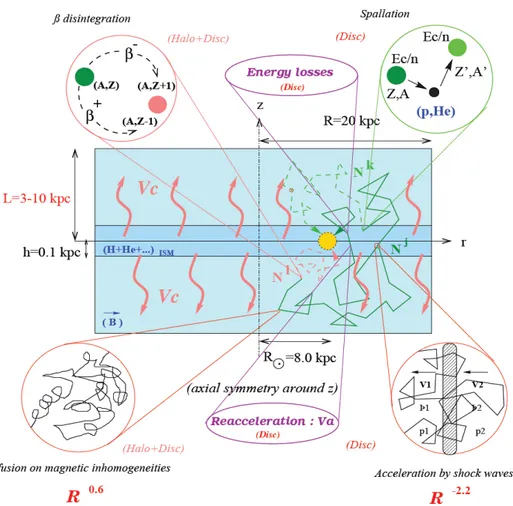
The CR propagation in the Galaxy is dominated by particle motion in the galactic magnetic field and through ionized gas that together form a magnetic-hydrodynamic fluid (MHD). Cosmic rays move in helical trajectories around the large scale field lines and interact with its small irregularities (Alfvén waves), that act as collisionless scat-tering centers. The galactic magnetic field extends out of the disk in a larger halo that designs the region where the diffusion takes place. Therefore a cosmic ray particle, in its travel from source to Earth, may accede to regions where the propagation condi-tions are different. Thus, a complete treatment of cosmic ray transport, has to consider diffusion in the full magnetic halo region. The CR propagation is generally described by a transport equation which includes source distribution, particle diffusion in the galactic magnetic field, energy losses, nuclear interactions, decays and acceleration processes. Hereafter kinetic energy per nucleon will be used (just energy for short). The most known formulation was proposed by the Ginzburg-Syrovatskii [15] with the following transport equation:

∂Nj ∂t =∇·(D∇Nj)−∇·(VCNj)− ∂ ∂Ej [bj(E)Nj(E)]−pjNj+ X k>j [Nk·pk→j]+Qj(E, r, t) (2.23) Many physical processes are contained in the equation. The physical meaning for the various terms is outlined as follows:

• CR Density

Nj(E, r, t)is the density of particles of jth kind, and is defined as

Nj(E, r, t) =

1 ν

Z

φj(E, r, t, ˆω)· dΩ (2.24)

Here φj(E, r, t, ˆω) is the cosmic ray flux in the ˆω direction and dΩ is the solid

angle element. • Diffusion

par-ticles in the turbulent magnetic field. The process is governed by the diffusion coefficient D. A common simplified parametrization for the diffusion coefficient D is

D = 1

3λDν (2.25)

where ν is the particle velocity and λD is the diffusion mean free path.

• Convection

The particle convection in a galactic wind with velocity VC is described in the

second right term of the equation. CR may not only diffuse in our Galaxy, they can also be carried by magnetohydrodynamic waves. The effect of this galactic wind is to dilute the energy of the particles located in the disk in a larger vol-ume, so that the adiabatic expansion results in a kind of energy loss (adiabatic deceleration), depending on the wind velocity VC = VC(t, r).

• Energy losses

The third right term of the equation represents the continuous energy losses bj(E) = −

dE

dt (2.26)

expresses the mean rate at which the particle j changes their energy. The only processes relevant for nuclei are ionization and Coulomb losses in ionized plasma. Other effects like bremsstrahlung, inverse Compton and synchrotron radiation are important only for light particles (e±_).

• Decay and break up

The term pjNj represents the destruction rate due to collision and decay with

pj = nνσj +

1

γτj (2.27)

where τj is the lifetime of nucleus j for radioactive decay. The interstellar gas

(hydrogen and helium) density is parametrized with n = n(x) and σj is the total

inelastic cross section for the processes Nj + ISM −→ anything.

• Spallation

The sum Pk describes the production of type j nuclei from interactions of

dif-ferent types k nuclei. Only heavier nuclei (k > j) are usually considered in the sum. The process probability is also given in terms of production cross sections σk→j ≡ σ(Nk+ ISM −→ Nj+ anything) as

Pj = nβcσk→j+

1

where the contribution from heavier radioactive nuclei k to the nuclear channel j is also considered. No energy migration Ek −→ Ej is considered in this term,

as long as kinetic energy per nucleon is conserved in spallation. This is the main reason why theoretical models use the kinetic energy per nucleon as a fundamental quantity.

• Source distribution

Last term in the equation is the primary source term. In the most general case it may be time and space dependent, even though stationarity and cylindrical symmetry are often invoked to simplify the problem.

Solving the transport equation requires the complete analysis of a system of coupled equations. Together with the possibility of working out an analytical/numerical solu-tion, an assumption that all the parameters are well known or needed to be known is mandatory, and additional assumptions have to be done for defining the boundary conditions for the equation. Hence, different models of CR propagation in the Galaxy can be represented using the equation written above, with specific boundary condi-tions and approximacondi-tions. Three often used propagation models are presented in the following: the Diffusion Halo Model (DHM), the Weighted Slab Model (WSM) and the Leaky Box Model (LBM).

2.3.1

Diffusion Halo Model

The most realistic physical scenario for CR propagation is a diffusion model in which the diffusion-transport equation is solved by taking into consideration all the physical processes, involved together with observational physical constraints, such as cosmic rays nuclear ratios[18]. This physical constraints generally assume that cosmic ray sources are placed in the thin galactic disc, where most of the interstellar gas is located. Cosmic rays are assumed free to diffuse out, in the whole halo region, where they are able to spend considerable portion of their lifetime. Escaping the halo is also allowed and out of the considered region the CR density becomes zero. Since cosmic rays travel with relativistic speed, the long residence time requires that they cannot move rectilinear to outer space: during this period they undergo many scatterings, without loosing too much energy, and interact with gas, producing secondary particles. This way, using light nuclei ratios, we can fix some parameters and then improve the accuracy of some software (e.g. Galprop) to obtain numerical solutions for cosmic rays propagation[24,25]. As already mentioned, this model predicts a CR diffusion toward

46

Spatial diffusion: It has been assumed to be isotropic. Actually, the diffusion coefficient K should

be replaced by a tensor, with parallel and transverse components. As regards the first one, there is

a strong consensus about a form

where 𝜅 is the spectral index of the turbulence spectrum, and the normalization K

and the

spectral index 2 − 𝜅 = 𝛿 should ideally be related to the astrophysical properties of the

interstellar medium. β  is  1  for  ultrarelatistic  particles.  Unfortunately, our knowledge in this field is

still demanding, and the value of the two parameters K

and δ can only be determined indirectly

by the analysis of cosmic ray observations [142].

Geometry: The propagation of cosmic rays ceases to be of diffusive nature beyond some surface

where they can freely stream out of the diffusive volume. The density then drops to nearly zero,

so that this surface may be considered as an absorbing boundary. The exact shape and dimensions

of this boundary are not known, but direct observations of the radio halo of external galaxies

suggest that it might radially follow the galactic disc, with a greater thickness. Embedded in this

diffusive halo lies the disc containing the stars and the gas . The gas is mostly made of hydrogen

(90%), neutral and ionized, and helium (10%) (the heavier nuclei that may be present are of

negligible importance). The different components, stars and gas, have different half heights of the

order of h ∼ 100 pc; so they all satisfy h ≪ L, so that the disc will be considered as infinitely thin

for all practical purposes. Sources and interactions with matter are confined to the thin disc and

diffusion which occurs throughout disc and halo with the same strength, is independent of space

coordinates. The Solar System is located in the galactic disc (z = 0) and at a Galactocentric distance

R

= 8.5 kpc . A schematic view of the galactic model is shown in Fig. 4.

Figure 4 - Schematic view of our Galaxy as well as all propagation steps included in the diffusive

model.

Energy losses from interaction with the ISM: There are two types of energy losses which are

relevant for nuclei: ionization losses in the ISM neutral matter and Coulomb energy losses in a

completely ionized plasma, dominated by scattering off the thermal electrons. The other effects

(3.22)

Figure 2.11: Schematical view of the Galaxy with CR propagation steps in a diffusive halo model context[95].

the halo, that means that there is a gradient of CR density away from the galactic disk. Consequently, a constant streaming of CR particles is produced. This streaming is determined by the energy dependence of the diffusion coefficient D(E) and the halo size.

Solutions for the transport equation,written according to this model, can be expressed using the Bessel series expansion, assuming a cylindrical symmetry for the galactic halo, as ψ(E, r, z) = ∞ X i=1 Pi(z, E)J0( αir R ) (2.29) where φ = dN

dE is the distribution function, J0 is the zero order Bessel function and goes

to zero for αi, Pi are the Fourier transform using cylindrical coordinates and R is the

cylindrical radius. The basic quantities exploited to develop the model are explained in detail in the following:

• Geometry of the Halo Model:

ob-servation done using the radio halo of external galaxies, suggest that it could be considered as an infinitely thin disc (h ' 100 pc, R ' 20 kpc and h  L) containing stars and gas (90 % H and 10 % He), followed by a radially expanded halo with a greater thickness. Sources and interactions are confined to the thin disk and diffusion takes place indipendently respect to space coordinates. The Solar System is located in the galactic disk at z = 0 and at a distance ' 8.5 kpc from the center of the system (see Fig. 2.11).

• Gas distribution:

The spatial density and composition of the interstellar gas (ISM) is a rather homogeneous mixture of hydrogen, helium, ionized gas and dust located in a narrow disk with average density of ' 1 particle/cm3 _[17].

• Source distribution:

The most common used source spatial distribution is flat (Q(r) = 1) or radial distribution Q(r) ∝√r·e1−r0r , with r_{0 = 8.5}kpc. However, the difference between

a flat and a radial distribution is a mere rescaling of the propagation parameter, i.e. not significant if one consider these parameters as effective in a consistent framework [18,19]. The source energy spectrum is determined by the acceleration processes at work. There is a strong belief that this spectrum is a power law in rigidity Q(r) ∝ R−α_.

• Diffusion coefficient:

Considering an isotropic diffusion, a good approximation for the diffusion coef-ficient is a constant function of the space coordinates, or at least a two value function for diffusion in the disk and in the halo. Its energy dependence is usually expressed as a power law in rigidity D = K0βR2−κ, where κ is the spectral index

of the turbolence spectrum, K0 is a normalization constant and δ = 2 − κ is a

redefinition of the spectral index. The last two parameters are both related to the ISM properties and are determinated indirectly using CR observations[26]. • Reacceleration:

Since in real astrophysics environment propagation can be more complex than a simple diffusion, reacceleration of CR particles can also be included. This accel-eration is continuous and due to magnetic field inhomogeneities (see Fig. 2.12). The process can be studied in terms of a diffusion in momentum space, provided that the hydromagnetic turbulence may be regarded as homogeneous, and time

A.Morselli 13 - 6 - 2008 GALPROP tutorial 83

Distributed Stochastic Reacceleration

Fermi 2-nd order mechanism

B

B

Scattering on magnetic

turbulences

D

~ p

_V

/D

D ~ vR

_-

_{Kolmogorov spectrum}

I

E

strong

reacceleration

weak

reacceleration

ΔE

Simon et al. 1986

Seo & Ptuskin 1994

1/3

D

= 5.2x10

_{(R/3 GV)}

_cm

_s

V

= 36 km s

γ

_{~ R}

_{, δ=1.8/2.4 below/above 4 GV}

Figure 2.12:Schematical view of the reacceleration process[186].

independent. This involves an additional term in the transport equation: 1 p2 ∂ ∂p[p 2_D pp ∂Nj ∂p ] (2.30)

where Dpp is the diffusion coefficient that acts in the momentum space. If we

idealize the magnetized fluid elements as hard spheres with masses much larger than those of the particles, we can write Dpp for elastic collisions as:

Dpp=

V2 a

3λcβp

2 _(2.31)

where Va and cβ are respectively the velocities of the fluid elements (Alfvén

ve-locity) and particles, and λ is the mean free path against collisions with the fluid elements. The Alfvén velocity represents the velocity by which a perturbation in the magnetic field propagates along the magnetic field lines. Expressing the (spatial) diffusion coefficient as D = 1

3λDν, a relation between D and Dpp can

be established:

Dpp=

V2 ap2

9D (2.32)

• Energy losses from interaction between nuclei and ISM:

There are three kind of energy losses that are important for CR nuclei: Coulomb energy losses in a ionized plasma, dominated by scattering off the thermal elec-trons, ionization losses in the ISM neutral matter and adiabatic losses from convective (or galactic) wind. The Coulomb energy losses can be written as

(dE dt )coul≈ −4πr 2 emec2Z2neln(∆ β2 x3 m+ β3 ) (2.33)

where re and me are respectively the electron radius and mass, ne ' 0.33cm−3

is the interstellar electron density, Z and M are charge and mass number for incoming nuclei and ln∆ ' 40 ÷ 50 is the Coulomb logarithm.

The relativistic expression for ionization losses can be written as (dE dt )ion ≈ − 2πr2 emec3Z2 β X s=H,He nsBs (2.34) where Bs≡ ln( 2mec2β2γ2Qmax I2 s )_{− 2β}2 (2.35) and Qmax ≡ 2mec2β2γ2 1 + [2γme/M ] (2.36)

where Is is the excitation/ionization mean potential of the considered atom,

M  me is the incident nucleon mass and ns is the density of the target atom

in the ISM. As already run over, among the phenomena affecting the CR propa-gation there’s the effect induced by the medium as it moves away from the disk with a velocity VC. This mechanism is called convective or galactic wind and

its main effect is to dilute the energy of the particle located in the disk into a larger volume, this adiabatic expansion results in a third type of energy loss that depends on ∇ · VC. This wind, that occours only on the galactic disk, is

considered to be perpendicular to the disk plane and to have a constant magni-tude throughout the diffusive volume. The energy loss due to this process can be written as (dE dt )adiab =−Ek( 2m + Ek m + Ek )VC 3h (2.37)

• Galactic magnetic field:

According to radio synchrotron, optical polarization and Zeeman splitting data, the galactic magnetic field is composed of two components: a regular one with an average value of few µG that is parallel to the galactic plane and responsible for confinement, and a stochastic one which is responsible for charged nuclei diffusion and has about the same intensity as the previous one[27]. The average strength of the total magnetic field in the Milky Way is about 6 µG near the Sun and increases to 20-40 µG in the Galactic center region. The overall field structure follows the optical spiral arms and a radial distribution is a good approximation for it[17].

• Solar modulation:

cavity, a process by which they lose energy. This phenomenon is called Solar modulation and may be pictured as follows. The Sun emits low energy particles in the form of a fully ionized plasma having v ' 400kms−1 _{, mainly electrons and}

protons with E ' 0.5 MeV. Once the plasma has left the corona, the dynamic pressure dominates over the magnetic pressure through most of the Solar System, so that the magnetic field lines are driven out by the plasma. The combination of the outflowing particles motion with the Sun’s rotation leads to a spiral pattern for the flow. This Solar wind shields the Solar cavity from penetration of low energy CR. The region of space in which the solar wind is dominant is called heliosphere. The charged particles that penetrate the heliosphere are diffused and energetically influenced by the expanding solar wind. As this effect involves all the cosmic rays that are detected at Earth (or in near space), it must be taken into account. For practical purposes it can be used the force field approximation [28,29,30]. The final result of this approximation is a shift in the total energy

ET OA A = EIS A − |Z| φ A (2.38)

where ET OA _{is the energy at the top of the atmosphere, E}IS _{is the total}

inter-stellar energy, Z and A are respectively the charge and atomic number of the nucleus and φ is the solar modulation parameter, its value varies according to the eleven years solar cycle ranging between 300 ÷ 1500 MV, and its determination is totally phenomenological.

• Geomagnetic cut − off:

The last obstacle for cosmic rays before being detected by an Earth orbiting detector is the Earth magnetosphere, that extends its influence on the cosmic radiation modulating the low energy part of the observed spectra (up to ' 15÷20 GV of rigidity). To first approximation, the geomagnetic field can be represented as an offset and tilted dipole field with moment M = 8.1·1025 _{G· cm}3_{, an}

in-clination of 11◦ _{to the Earth rotation axis and a displacement of about 400 km}

with respect to the Earth center. Because of the offset, the geomagnetic field, for a fixed altitude from the ground, is characterized by distortion, the high-est of which is in the South Atlantic, where the field strength is the weakhigh-est. The charged particles penetrate deeper in this region and the radiation becomes stronger. This high radiation phenomenon (Fig. 2.13) is the so called South At-lantic Anomaly (SAA). The most important aspect for CR measurements is the determination of the geomagnetic cut-off, as it prevents CR from reaching the detector: it is maximum at the geomagnetic equator (' 15 GV) and vanishes at

50

Figure 5 - Interstellar (black) and solar modulated (red) proton spectrum [74]. LIS stands for Local Interstellar spectrum (100 MeV-10 GeV energy range) [390].

Earth Magnetosphere

The last obstacle for cosmic rays before being detected by an Earth orbiting detector is the Earth magnetosphere, that extends its influence on the cosmic radiation modulating the low-energy part of the observed spectra (up to  15÷20 GV of rigidity).

To first approximation, the geomagnetic field can be represented as an offset and tilted dipole field with moment M = 8.1·1025 Gcm3, an inclination of 11° to the axis of Earth rotation and a displacement of about 400 km with respect to the Earth center. Because of the offset, the geomagnetic field, for a fixed altitude from the ground, is characterized by distortion, the highest of which is in the South Atlantic, where the field strength is the weakest. The charged particles penetrate deeper in this region and the radiation becomes stronger. This high radiation phenomenon (Fig.6) is the so called South Atlantic Anomaly (SAA).

Figure 6 – The SAA (red) projected on the geographic surface with a relative CR particle rate. The SAA is the area where the Earth's inner Van Allen radiation belt comes closest to the Earth's surface dipping down to an altitude of 200km, leading to an increased flux of energetic particles [75, 294]. The SAA magnetic field worth 25000 nT against the normal value of 45000 nT [392].

Figure 2.13: Chromatic view of the south atlantic anomaly projected on the Earth surface, the color is related to CR rate[38].

poles.

2.3.2

Weighted Slab Model

The principal idea of the weighted slab model is to choose a geometry for the Galaxy and to replace the time and space dependence of the fluxes in terms of matter thickness traversed [22]. In this model the abundance of a nuclear or particle species depends on the inelastic collisions between particles and ISM and on the production rate due to the spallation with heavier nuclei [3]. It is convenient to introduce the density of matter traversed by the particle x = ρl, expressed in g · cm2 _{and called grammage.}

Nuclei of the same species with a given energy do not have necessarily the same propagation history, so that a probability distribution of grammage is associated with all the species; the function G(x), called path length distribution, is then introduced. G(x)is the probability that a nucleus j has crossed the grammage x. The corresponding density Nj is given by:

Nj =

Z ∞ 0

˜

Nj(x)· G(x) dx (2.39)

where the unweighted functions ˜Nj are the CR densities after traversing a matter

slab with thickness x. Since the grammage is directly related to the destruction rate and corresponding cross sections (total σj and partials σkj ), the ˜Nj can be simply

determined from the equation: d ˜Nj dx = 1 ¯ m[ X k>j (σk→jNk)− σj] (2.40)

where ¯m is the average ISM mass and the initial condition ˜Nj(0) = Qj(E) must be

imposed. In WSM framework the G(x) function is derived empirically, in order to account for data, and all information on the CR propagation have then to be inferred in terms of grammage. The G(x) can also be determined through the choice of the propagation model, in this sense the WSM represents a general technique. Indeed the grammage can be used in any propagation equation (DHM, LBM) [24]. For instance, inserting Eq.(2.20) into the transport equation leads to:

nβc∂G

∂x − ∇ · (D∇G) = f(r, t) · δ(x) (2.41)

which describes the propagation for point-like sources δ(x) spatially distributed ac-cording to f(r, t) (convection and energy losses are neglected here). The CR densities Nj are then given by Eq.(2.20), more precisely:

Nj(r) =

Z ∞ 0

˜

Nj(x)· G(r, x) · dx (2.42)

where the separation between the nuclear part Nj(x)and the astrophysical part G(r, x)

is apparent. This model is quite satisfactory in the high energy limit and for a particle-independent diffusion coefficient, where it becomes equivalent to the direct solution of the diffusion equation (2.21). It is also easy adaptable for every geometrical model of the Galaxy and for all spatial source distributions. The WLB allows to link Leaky Box Model (LBM) with more realistic descriptions, explaining why LBM works so well.

2.3.3

Leaky Box Model

The Leaky Box Model, introduced in the sixties and today still largely used, can be viewed as a further simplified version of the WSM, i.e. an extremely simplified ver-sion of the diffuver-sion model. The basic assumption is that diffuver-sion takes places rather rapidly. The distribution of cosmic rays in the whole box (i.e. Galaxy) is homoge-neous, they are free to propagate in the Galaxy with a certain escape time from the system. The production rate from the sources and the escaping rate allow to maintain a stationary flux in the Galaxy[3]. Starting from the WSM formulation (Eq. 2.22), it consists in the substitutions:

∇ · (D∇Nj)↔

Nj

where τesc is the escape time of cosmic rays from the Galaxy, and with the average of

every quantities (e.g. n ↔ ¯n). The result is the basic LBM equation: ∂Nj ∂t = Qj − Nj τesc − ¯nβcσj Nj + X k>j [¯nβcσk→jNj] (2.44)

The characteristic escape time τesc has to be determined experimentally and it is

a purely phenomenological quantity. In this model, other energy changing processes and convection are neglected. The physical interpretation of the LBM is that cosmic rays move freely in a containment volume, with a constant probability per time unit P = τ−1

esc. The number of escaped particles per unit time is proportional to the number

of particles present in the box. The other processes (decays, break up and spallation) may also be viewed in terms of characteristic times:

τ_intj = ¯n· βc · σjτintk→j = ¯n· βc · σk→j (2.45)

For steady state solutions dNj

dt = 0, the resulting equation system for the various nuclei

j are purely algebraic:

Nj τesc + Nj τ_intj = Qj+ X k>j Nk τ_intk→j (2.46)

The characteristic time τesc is often replaced by λesc, which characterizes the amount

of matter traversed by CR before escaping from the ISM:

λesc = ¯m· ¯n · βc · τesc (2.47)

where ¯n refers to the mean interstellar gas density through which the particle pen-etrates, ¯m means the mean mass of the gas, and βc is the velocity of the particle. Analogous substitutions can be done for τj

intand τ k→j

int , providing the mean interaction

lengths for decay or break up λj

intand fragmentation λ kj

int. As these latter processes are

obviously particle dependent, it should be noted that the escape time or length is the same for all the nuclear species, i.e. this formulation assumes that all nuclei have the same propagation history. Clearly this model is only an approximation which does not give indications of the main physical processes. Despite the simplicity of its physical framework, the LBM permits a direct analysis of flux measurements in function of only three fundamental parameters: the escape time, the mean matter density and the source abundances. This is largely sufficient for many purposes, because it reproduces very well the main observed features of secondary to primary CR ratios.

2.4 Cosmic Rays at the Top of the Atmosphere

At the final stage of their travel toward the Earth, cosmic rays are influenced by two local phenomena: the solar wind, which composes the heliosphere and extends up

to the boundaries of the Solar System, and the geomagnetic field, which is present in the Earth magnetosphere. Both the effects produce a distortion of the interstellar spectra measured at Earth. Two different approaches are traditionally followed by the CR physics community for these two phenomena. The solar wind influence on CR is studied by the theoretical community as well as other propagation aspects, i.e. the experimental measurements are usually presented uncorrected for this effect. Thus, low energy measurements are not representative of interstellar flux, and, since the solar wind varies with a eleven year timescale, experimental data coming from dif-ferent epochs are not directly comparable unless solar modulation is accounted. On the contrary, the geomagnetic modulation is considered as part of the experimental conditions: take into account this effect is responsibility of experimentalists. Measured fluxes must therefore be corrected in order to quote the geomagnetically demodulated spectra.

The Geo Magnetic Field (GMF) extends its influence on the cosmic radiation modulat-ing the low energy part of the observed spectra (≤ 10 GeV/n). In first approximation, as already mentioned, the GMF can be represented as an offset and tilted dipole field with moment M = 8.1 · 1025 _{G· cm}3_{, an inclination of 11}◦ _{to the Earth rotation axis}

and a displacement of about 400 km with respect to the Earth center. Charged parti-cles traversing the magnetic field experience the Lorentz force that produces a curved path for low rigidity particles. Cosmic rays can thus be prevented form reaching the detector, depending on their rigidity and incoming direction [33,35]. For a CR particle directed toward the Earth, the screening is determined by its rigidity, the detector location in the GMF and its incoming direction with respect to the field. Conversely, for given arrival direction and location, there will exist a minimum value of the par-ticle rigidity RC for which galactic CR are allowed to penetrate the magnetosphere

and be detected. In the dipole approximation, the rigidity cut-off RC was analytically evaluated by Stormer [36] that found the relation:

RC =

M cos4_λ

R2

e[1 + (1± cos3λ cos φ sin ξ)1/2]2

(2.48) where M is the dipole moment. The arrival direction is defined by ξ and φ, respectively the polar angle from local zenith and the azimuthal angle. The ± sign applies to nega-tively/positively charged particles. The arrival location is defined by the geomagnetic coordinates (R, λ), a commonly used coordinate system relative to the dipole axis, where R is the distance from the dipole center, usually expressed in Earth radii units (R = r/R⊕), and λ is the latitude along the dipole. These quantities come from the

simple dipole field description, where the components of the field are: Br =− M r32 sin λBλ = M r3 cos λ (2.49)

and the field lines have the form r ∝ cos2_{λ. For vertical incidence (ξ = 0) the azimuthal}

dependence of the cut-off simply vanished, putting in evidence the cutoff behaviour as a function of the geomagnetic latitude:

RV C =

M 4R2 cos

4_λ

≡ M_R20 cos4λ (2.50)

where M0 = 15if RV C is measured in GV . The cut-off is maximum at the geomagnetic

equator, with a value of approximately 15 GV, and vanishes at the poles. A more

Chapter 1. Cosmic Rays in the Galaxy

1.3. Cosmic Rays Near Earth

behaviour as a function of the geomagnetic latitude:

R

=

M

4R

cos

4

_λ

≡

M0

_R

cos

λ

(1.30)

where M0

= 15 if RV C

is measured in GV . The cut-off is maximum at the

geomag-netic equator, with a value of approximately 15 GV , and vanishes at the poles.

-90 -60 -30 0 30 60 90 -180 -150 -120 -90 -60 -30 0 30 60 90 120 150 180 Longitude Latitude

SAA

Figure 1.8:

lines are the magnetic field strength at the Earth surface. The red (blue) lines are the magnetic latitude (longitude). The SAA region is marked in this figure.

A more precise description of the cut-off can be obtained by replacing the dipole

coordinates with the Corrected GeoMagnetic coordinates (CGM). The method

con-sists in defining an opportune transformation GM

_{↔ CGM that maps a more}

re-alistic GMF model into the dipole representation [35]. The most commonly used

GMF model is the IGRF one. In this picture, a rather complex magnetic field B is

treated as the derivative of a scalar potential V , B =

_{−∇V , with V expressed by a}

series of spherical harmonics [36]:

V = R

!

"

R

r

#n+1

_!

P

(cos θ) (g

cos mψ + h

sin mψ)

(1.31)

where R

is the mean earth radius 6321.2 km, r is the geocentric radius, θ is the

geographic colatitude and ψ is the East longitude from Greenwich. P

(cos θ) are

the Legendre polynomial functions, g

n

and h

are the Gaussian coefficients that

specify the GMF, determined experimentally. The IGRF model is widely used in

geophysics and contains coefficients up to order 12. The dominant terms in Eq.1.31

are related to n = 1 that leads to the simple dipole field.

Figure 2.14: The CGM coordinate grid projected onto the geodetic map. The green contour lines are the magnetic field strength at the Earth surface. The red (blue) lines are the magnetic latitude (longitude). The SAA region is marked[187].

precise description of the cut-off can be obtained by replacing the dipole coordinates with the Corrected Geo Magnetic coordinates (CGM). The method consists in defining an opportune transformation GM ↔ CGM that maps a more realistic GMF model into the dipole representation. The most commonly used GMF model is the IGRF one. In this picture, a rather complex magnetic field B is treated as the derivative of a scalar potential V , B = −∇V , with V expressed by a series of spherical harmonics [33]: V = R⊕ ∞ X n=0 (R⊕ r ) n+1 n X m=0

P_nm(cos θ)(gm_n cos mφ + hm_n cos mφ) (2.51) where R⊕ is the mean Earth radius R⊕ = 6321.2 km, r is the geocentric radius, θ

is the geographic colatitude and φ is the East longitude from Greenwich. Pm n (cos θ)

are the Legendre polynomial functions, gm

n and hmn are the Gaussian coefficients that

specify the GMF and are determined experimentally. The IGRF model is widely used in geophysics and contains coefficients up to order 12. The dominant terms in the last equation are related to n=1 that leads to the simple dipole field. The corresponding CGM coordinates are illustrated in Fig. 2.14. This procedure allows to use the last two equations in a IGRF framework to estimate the effective exposure time of a detector to galactic cosmic rays.

Chapter 3

Dark Matter Physics

Galaxies are gravitationally bound system made of stars, gas and dark matter, an important but poorly understood component. Here gravity is the main force so that galaxies can be studied as N-interacting body systems. According to Hubble morpho-logical classification, galaxies can be splitted in three main groups: elliptical shape, spiral or irregular. Spiral shape galaxies are composed of two main parts: a central spherical or elliptical swelling (bulge) and the disk namely a flat asymmetric distri-bution of rotating material. Using the "Doppler shift" associated to absorbtion and emission lines of known electromagnetic wavelengths, one can estimate the motion along the line of sight for stars and gas in the disk with a relative velocity v. In the case of not relativistic radial velocity (vrad) one can observe the wavelength λobs [57]:

λobs − λem

λem '

vrad

c (3.1)

Here λem is the hyperfine line emitted by the neutral hydrogen at 21 cm, associated to

the transition from a spin 1 state (alignment of proton and electron spins) to a spin 0 state (opposite alignment of proton and electron spins). The main effect of rotation is the wavelength shift. If we now assume a circular orbit, the resulting rotation velocity turns out to be:

vc=

vrad− vs

sin i (3.2)

where vs is Galaxy center of mass velocity and i is the angle between the line of sight

and the perpendicular to the disk [57]. The variation of vc relative to the galactic

radius can be used to measure the mass profile of the Galaxy and can be expressed through a rotation curve (see Fig. 3.1). Using the centripetal acceleration definition, in the spherical case we obtain the following relation:

v2_c = GM (r)

where M(r) is the mass contained in a sphere with a radius r and G is the gravita-tional constant. In particular the star mass can be studied using the ratio M

L, through

luminosity (L) measurements, while the gas mass can be determined through the mea-sure of neutral hydrogen (NI). Usually in spiral galaxies the star contribution to the total mass is greater than the one from the gas, so that beyond the optic radius the above relation reduces to vc ∝ r−1/2. However observations show that when r increases

vc ' const: this can be explained invoking the presence of a dark matter halo in the

region far from the center, with a density ρ ' r−2 _{and mass M ∝ r, or using an}

al-ternative gravitational theory. In the first case, still considering a spiral shape Galaxy, the dark matter composition should be five to ten times the baryonic composition, in the other case we should consider a modified gravitation theory for an acceleration less then 1.2 · 10−10 _m/s2_.

Figure 3.1: Rotational curve for the NGC3198 galalxy. Here vcfor gas and stars is expressed

in function of the distance from the center R[58].

3.1 ΛCDM Model

Cosmology is the branch of Physics devoted to the study of Universe evolution from the Big Bang until nowadays. Cosmology is found on two main principles:

• The Cosmological Principle:

according to this the Universe can be considered homogeneous and isotropic on a large scale. The Universe homogeneity can be applied only considering extended parts of it, locally this assumption is uncorrect, but it works if we consider spatial regions larger then 108 _{ly. According to actual cosmological models, Universe}

can be considered as an ideal fluid and each Galaxy can be located using a set of coordinates xµ _{= (t, r, θ, φ), the quadri-velocity associated to the Galaxy is}

uµ _{= (1, 0, 0, 0) and u}µ_uν _{= g}

µν = g00 = 1, here gµν is the metric tensor. In this

• The Equivalence Principle:

according to this second principle, if we fix a point in the space-time framework and an arbitrary gravitational field, we can always find a locally inertial reference system, so that near this point physical laws are those of special relativity [44]. Choosing the first principle we can use a coordinate system (t, r, θ, φ), in this system the metric can be expressed as:

ds2 = dt2_{− R}2(t)[ dr

2

1_{− kr}2 + r

2_dθ2_{+ r}2_{sin θ}2_dφ2_{] (3.4)}

that is the Robertson-Walker metric. Here we consider c = 1, k is a constant with three posible values (-1,0,1), R(t) is a scale factor when k=-1,0, it is the Universe radius when k=1. When k=0,-1 the Universe is considered as infinitely extended, when k=1 it is characterized by a circumference L = 2πR(t) and a volume V = 2π2_R3 _[39].

3.1.1

Friedmann Equations

We can obtain the Friedmann equations using the Robertson-Walker metric written above (Eq.3.4) along with the Einstein equation that can be written as follow[40]:

Rµν −

1

2gµνR =−8πGTµν (3.5)

where Tµν is the energy-momentum tensor and Rµν is the Ricci tensor i.e. the

contrac-tion between the Riemann tensor with the metric tensor. Introducing in the precedent equation the term

Sµν = (Tµν − 1 2gµνT λ λ) (3.6) we obtain Rµν =−8GSµν (3.7)

In our case the energy-momentum tensor is the one for ideal fluid:

Tµν =−p(t)gµν+ (p(t) + ρ(t))uµuν (3.8)

here p is the fluid pressure and ρ the fluid density, both time dependent. Using this energy-momentum tensor we can rewrite Sµν as:

Sµν =

1

2(p− ρ)gµν + (p + ρ)uµuν (3.9)

Substituting the Robertson-Walker metric we obtain: S00 = 1 2(ρ + 3p)S0i= 0Sij = 1 2(p− ρ)R 2_(t)g ij (3.10)

where gij = 0when i 6= j, g11 = (1− kr2)−1, g22 = r2, g33 = r2sin θ2. The terms in the

Ricci tensor that differ from zero are R00=

3 ¨R

R R0i= 0Rij =−(R ¨R + 2 ¨R

2_{+ 2k)g}

ij (3.11)

Combining these three relations with Sij we obtain:

3 ¨R = −4πG(3p + ρ)RR ¨R + 2 ˙R2+ 2k = 4πG(ρ− p)R2 _(3.12)

Substituting the first in the second we finally obtain Friedmann equations: ˙ R2_{+ k =} 8πGρR2 3 ¨ R R =− 4πG(3p + ρ) 3 (3.13)

Considering the conservation of the energy-momentum tensor we obtain a third equa-tion that is:

d(ρR3₎

dR =−3pR

2 _(3.14)

We can also introduce a useful parameter that is the Hubble constant H(t) = R˙

R (3.15)

using it we can express the linear relation between the redshift associated to the Galaxy light emitted (z) and its distance (d):

cz = H0d (3.16)

here H0 is the Hubble constant and its value is 67, 3 ± 1, 2 km/s/Mpc[181].

3.1.2

Universe Classification

Let’s go back to the first Friedmann equation: ˙

R2+ k = 8πGρR

2

3 (3.17)

if we now consider k=0, as suggested by experimental results, we obtain a value for critical density, that is:

ρc=

3H2

8πG ' 1, 88 · 10

−29_g/cm3_{h (3.18)}

Using this critical density we can define the ratio Ω = ρi

where ρi is the source energy density we consider. From this relation one can obtain, by

summing up the different contributions, the total amount of energy density Ω. Using Ωwe can learn about the Universe curvature and distinguish between three cases[40]:

Ω > 1→ ρ > ρc→ k = 1 (3.20)

Ω = 1→ ρ = ρc→ k = 0 (3.21)

Ω < 1_{→ ρ < ρ}c→ k = −1 (3.22)

Considering now the second Friedmann equation ¨

R R =−

4πG(3p + ρ)

3 (3.23)

given that the term (3p + ρ) is positive, it follows that ¨R < 0 so that we can con-clude the Universe to be in decelerate expansion. Nevertheless in 1999, two different and indipendent studies [40,41] highlighted that the Universe expansion is accelerated [40,41]. The theoretical way to insert in our cosmological model this expansion is to consider an additional term (Λ) in Einstein equation:

Rµν −

1

2gµνR− Λgµν =−8πGTµν (3.24)

here the new term Λ is the cosmological constant. Considering this additional contri-bution to the energy density we obtain

Ω = Ωm+ ΩΛ+ ΩR+ Ωk (3.25)

where Ωm is the matter density, Ωk is the density associated to curvature and ΩR is

the radiation density. Using the cosmic microwave background radiation (CMB), some values for these densities have been determined:

ΩR ' 0 (3.26) Ωk' 0 (3.27) Ωm ' 0, 315 (3.28) ΩΛ' 0, 686 (3.29) so that Ω = 1, 001 (3.30)

To explain such a result, we have to introduce an extra contribution to the total energy density, that is