A Language-based Approach to Distributed Resources

(1)

Universit`a di Pisa

Dipartimento di Informatica

Dottorato di Ricerca in Informatica

INF 01

Ph.D. Thesis

A Language-based Approach to

Distributed Resources

Viet Dung Dinh

Supervisors Prof. Chiara Bodei Prof. Gian Luigi Ferrari

Referees Prof. Ant´onio Ravara

Dr. Emilio Tuosto

Chair

Prof. Pierpaolo Degano

(2)

(3)

Abstract

Modern computing paradigms for distributed applications advocate a strong control on shared resources available on demand in order to guarantee their correct usages. An illustrative example of such paradigms is Cloud Computing. In this dissertation, we study formal models for distributed applications, paying particular attention to resource usage analysis. Formal methods for specifying and analysing different as-pects of resource management could play an important role for the widespread usages of distributed resources. They provide not only the theoretical framework to un-derstand the stages underlying the design and implementation issues, but also the mathematically-based techniques for the specification and verifications of properties of such systems. In this dissertation, we introduce two models, called λ{}-calculus and G-Local π-calculus, which are extensions of λ-calculus and π-calculus respec-tively.

The λ{}-calculus is an extension of concurrent λ-calculus enriched with suitable mechanisms to express and enforce application-level security policies governing us-ages of resources available on demand in the clouds. We focus on the server side of cloud systems, by adopting a pro-active approach, where explicit security policies, which are expressed as a set of execution traces, regulate server’s behaviour. By providing an abstract cloud semantics, we ensure that enforcing security policies embedded in cloud applications is sound.

The G-Local π-calculus is built on top of the standard π-calculus by introducing new primitives to manage resources. Unlike the previous model, where resources are highly abstract, resources in this approach are modelled as stateful entities with local states and global policies. A high degree of loose coupling among applications and resources is achieved through the publish/subscribe model. Furthermore, we develop two static, language-based techniques, namely Control Flow Analysis (CFA) and Type and Effect Systems, to reason about resource usages and therefore able to predict bad usages of resources. The CFA mainly focuses on reachability properties related to resource usages. It computes an over-approximation of resource usages of applications. As a result, if the approximation does not contain bad usages, then it guarantees that applications correctly use resources. The type and effect system provides a closer view of resource behaviour. Resource behaviour is extracted in the form of side effect of the type system. We exploit side effect to verify regular linear time properties, expressed by Linear Time Logic formulas, of resource usages.

(4)

(5)

Acknowledgments

First of all, I would like to express my deepest gratitude to my supervisors, Prof. Chiara Bodei and Prof. Gian Luigi Ferrari, who guided me through technical issues of my work and helped me focus on research. I would have unable to complete this thesis without their support, lessons and patience.

I wish to thank my external reviewers, Prof. Ant´onio Ravara and Dr. Emilio Tuosto, for their valuable and detailed comments, and the thesis committee mem-bers, Prof. Antonio Brogi and Prof. Pierpaolo Degano, for their precious comments and suggestions.

I am indebted to my friends and colleagues An, Claudio, Dung, Giovanni, Hieu, Igor, Ha, Lopa, Luca, Lam, Mateo, Minh, Naveen, Peter, Rebecca and Rui, and to friends from my football team, Kim, Liem, Tim, The and Vu. With them, life in Pisa was far more enjoyable.

Finally, I would like to thank my parents and my sister for their love and support throughout my studies.

(6)

(7)

List of Figures

2.1 Transition systems of a mobile reader with a low-bandwidth (on the

left) and a high-bandwidth (on the right) connection . . . 23

2.2 The Operation Semantics of BPP processes. . . 30

2.3 The usage automata for the policy of the low-bandwidth connection . 39 2.4 The Operational Semantics of the λ[] . . . 39

2.5 Typing rules . . . 41

2.6 The operational semantics of CCS processes. . . 44

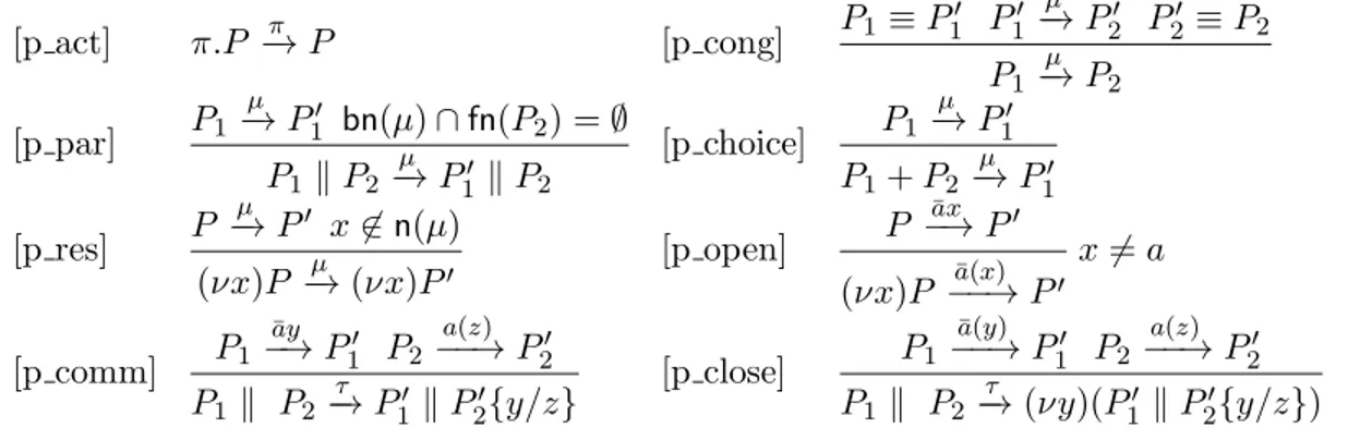
2.7 Structural Congruence. . . 46

2.8 The Operational Semantics of Processes. . . 47

3.1 Usage automaton of the service Q . . . 66

3.2 Cloud Semantics . . . 68

4.1 Structural congruence. . . 90

4.2 Operational Semantics of G-Local π processes. . . 91

4.3 The initial configuration of the robot scenario. . . 105

4.4 The policy automata of the robots’ families: R1 (left), R2 (middle) and R3 (right). . . 105

5.1 Structural congruence. . . 117

5.2 Operational Semantics of G-Local π processes. . . 118

5.3 Structural Congruence on Types . . . 120

5.4 Operational Semantics of Types. . . 120

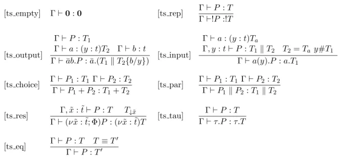
5.5 Typing rules. . . 123

(10)

(11)

List of Tables

2.1 BPP decidability . . . 31

2.2 Specification of 0-CFA . . . 35

2.3 CFA Equational Laws . . . 48

2.4 The Operational Semantics of Types . . . 53

2.5 The interpretation of formulae over terms . . . 55

2.6 The “hiding” operator on types . . . 55

2.7 Typing rules . . . 56

(12)

(13)

Chapter 1 Introduction

1.1 Motivations

Nowadays, the evolution of network infrastructures and computing technologies heavily impacts on the design of software applications. It is reflected by the shift from (traditional) applications running in a well-determined environment to dis-tributed applications running into a dynamic evolving environment. This trend has led to introducing or revising different computing paradigms such as Service-oriented Computing, Cloud Computing and Ubiquitous Computing. Service-oriented Com-puting [91] is based on the idea of providing a network of services, which are basically loosely-coupled basic computing entities. The network of services is exploited to cre-ate a flexible way to assemble services into effective applications. The advantage of having high performance network infrastructures allows to rapidly deploy and scale services at runtime, i.e. on-demand deployment. This is one of the key ideas of Cloud Computing [37]. Basically, cloud-based applications allow for an intensive usage of distributed resources. The integration of iCloud on Apple products, e.g. iOS and Mac OSX, to store/access information on cloud storage is an illustrative example of this trend. The promise of Ubiquitous Computing [109] is to embed “computing devices” into daily activities and let them work transparently to provide feedback or adjust themselves in accordance with novel configured settings. Close to Ubiquitous Computing is the idea of Internet of Things [7], where “things” or identifiable objects that are connected over the Internet are capable of gathering, processing, analysing information around them. The fact that applications in these visionary paradigms are able to access a variety of ubiquitous resources requires a development of a new framework to design and implement applications, where resource management is a central concern.

In this dissertation, we focus on the design of suitable mechanisms to control the distributed management of resources. Resources can be geographically distributed (possibly over continents) and independent, and could be accessed at any time from anywhere. The geographic distribution recalls the loosely coupled design

(14)

methodol-ogy of SOC. However, unlike SOC services, which are often autonomous and interact with users through pre-defined protocols (that is, users need to follow the proto-cols provided by SOC services), distributed resources are subjects to usage policies, provided that users must employ them correctly. The publish-subscribe paradigm assumes a notable role in this view. Indeed, the publish-subscribe paradigm is not only a natural choice to represent distributed resources, but it also emphasises the fact that resources have to be published by external parties and therefore have to be available to everyone through appropriate requests. This form of “plug and play” strongly requires suitable mechanisms to guarantee correctness of usages.

Understanding the foundations of the distributed management of resources could support state-of-the-art advances of programming language constructs, algorithms and reasoning techniques for resource-aware programming. In this perspective, for-mal methods for specifying and analysing system behaviours can offer an important support. On the one hand, they provide the theoretical framework to understand the stages underlying the design and the implementation issues of software sys-tems. On the other hand, they support the mathematically-based techniques for the specification and verifications of properties of such systems. Implementation of distributed applications with intensive resource usages in turn requires development of resource-aware programming languages. In other words, the programming model should have first-class primitives for resource management and able to describe in-teractions between resources and applications that use them.

In the last few years, many formalisms have been developed to manage resource usages. The focus of these research activities ( [11, 64, 19, 85], to mention only a few) is mainly on verifying abstract resource behaviour at a high level view, i.e. without an explicit model of resources. The high level abstraction of resources is often too general to describe a variety of resources. We believe that developing explicit models of resources is the first step for understanding resource behaviours. Resources should be modelled as independent entities with their states and properties that are subject to security policies. In this dissertation, we advocate the idea of history-based access control [1] to specify based properties of resources. Indeed, we think that trace-based approach equipped with suitable reasoning techniques allow us to smoothly verify resource usages.

Process calculi are a natural choice to model distributed resources. In the π-calculus, resources are just names. Behavioural types [63, 4] allow to express prop-erties of names related to distribution and concurrency. However, names them-selves are too abstract to express interesting properties, for instance, whether an application uses correctly resources or not. To address this, the works presented in [64, 19, 66] introduce an abstract model of resources in terms of execution traces. The works reported in [64, 19] abstract away resource management, while in [66] re-source management is provided by the semantics of private names. Alternatively, the work presented in [36] represents resources as sets of constraints: this choice allows one to represent service level agreement between users and resource providers. Still, this view does not guarantee the correctness of resource usages. The work reported

(15)

1.2. STRUCTURAL OPERATIONAL SEMANTICS 15

in [47] introduced a monoidal structure of resources, whose semantics is related to the sharing semantics provided by the binary operator in the monoid. However, co-evolution of processes and resources causes co-dependency, hence a rigid inter-action between processes and resources. We prefer for an alternative view, based on the idea of emphasising loosely coupling nature of interaction between resources and processes. The above discussion urges the need of a novel and innovative ap-proach to usages of distributed resources, which provides a more precise view of distributed-resource behaviour. We believe that the model has to support a loosely coupled design methodology and it provides a basis for verifying correctness of re-source usages.

The aim of this thesis is to bring together a variety of techniques to address issues arising in the new environment underpinned by the fast growth of network infrastructure and computing technologies. First, in our approach, resources are first class entities in the programming model and are explicitly modelled. Second, language-based techniques naturally permit to deal with resource-aware program-ming constructs. Third, language-based techniques allow one to establish a high level of abstraction not only for reasoning semantically on the behaviour of the whole system, but also for extracting properties of individual components, e.g. re-sources. Finally, we develop algorithms to verify correctness of resource usages, which is a primary concern in our approach.

1.2 Structural Operational Semantics

Understanding the precise semantics of programming languages plays an important role in the development of high-level programming languages. One of the main approaches to define formal semantics is operational semantics, introduced in the sixties [80, 77]. A main break through has been provided by Plotkin [93] with the introduction of so called structural operational semantics (SOS). SOS provides a way of describing the meaning of computing systems through a set of inference rules, which describe the evolution of the systems in a compositional manner. An inference rule is defined of the form:

promises conclusion

where if the premises are satisfied, so does the conclusion. In this way, SOS defines the meaning of a program in terms of the meaning of its parts, thus providing a structural, i.e., syntax-directed and inductive view of operational semantics.

SOS gives the basis for formal tools to statically analyse behaviours of computing systems due to its compositional nature. Rule-based syntax-directed approach for describing program behaviours in compositional manner gives a basis for proving properties of computing systems, that can be obtained or derived from properties of its components.

(16)

1.3 The λ-calculus

The λ-calculus was first introduced by Church during the 1930s as a formal system for studying computable recursive functions. Later, in the 1960s, Landin exploited the λ-calculus as the core mechanism of programming languages [74, 75]. Following Landin’s insight, the λ-calculus has been largely used in programming language design and implementation, and in the study of type systems. Its importance arises from the fact that it can be viewed simultaneously as a simple programming language (in the functional style) able to describe computations and as a mathematical object on which rigorous statements can be proved.

Despite its simple definition, the λ-calculus not only plays an important role in the development of programming languages, but it also finds application in many fields of computer science. One of the major applications is type theory. The simply typed λ-calculus, introduced in [46], provides a typed interpretation of the λ-calculus. The types, assigned to λ-elements, correspond to propositions in the intuitionistic logic via the type system, built on the simply typed λ-calculus. This correspondence is known under the name of Curry-Howard isomorphism. From the logic point of view, the proofs of logical formulas can be seen as programs, and therefore λ-elements. As a programming language, the formula that a program proves is the type of that program. By exploiting the dual view of the type system, one can specify properties of programs using logical formulas: the type system ensures that programs meet the required specification. From this point of view, type checking usually provide static guarantee: no error of a certain kind can occur at runtime.

1.4 Process Algebras

Process algebras provide a rather high level view of interactive systems, and a valu-able tool for specifying and analysing concurrent systems. Fundamental to process algebras is the parallel operator, allowing the decomposition of systems in terms of their concurrent components. Seminal process algebras are

• CCS, Milner’s Calculus of Communicating Systems [83], • CSP, Hoare’s Communicating Sequential Processes [34],

• ACP, Bergstra and Klop’s Algebra of Communicating Processes [21].

A number of extensions, based on these calculi, has been proposed to deal with various aspects of concurrency. In the π-calculus, in [84], a notion of mobility, i.e. dynamic change of the topological structure of processes, is presented. In [44], the locations or scopes of processes are exploited to handle administrative domains. Recently, applications of process algebras also exist to address issues in biology (see [95, 43]).

(17)

1.5. STATIC PROGRAM ANALYSIS 17

1.5 Static Program Analysis

Static program analysis is the analysis of software performed without actually exe-cuting programs. The analysis is applied to some version of the source code. Pro-gram analysis offers techniques for computing at compile-time, safe and efficient approximations of the set of configurations or behaviours arising dynamically, i.e. at run-time. By checking these approximations, one can verify several interesting prop-erties of programs. There are three major approaches to program analysis:

• Control Flow Analysis; • Abstract Interpretation; and • Type Systems.

Control Flow Analysis. Control Flow Analysis (CFA) has been introduced in the sixties [96]. CFA was mainly developed for functional languages [100, 65], but it found applications in other languages as well, for instance, in concurrent languages [26]. Basically, CFA provides a framework to compute which values or information can reach certain program points or can be assigned to a specific vari-able. The idea behind CFA is the specification of rules for transferring all possible information, from one program point to another. Thus, CFA usually gives an over-approximation of actual executions of programs. The correctness of programs is then guaranteed if no bad execution is found in the over-approximation.

Abstract Interpretation. Often, concrete and precise information about pro-gram properties is in general not computable within finite constraints in time and space. By abstracting the concrete semantics of computing systems, abstract pro-gram properties can be easily obtained to a certain degree of abstraction. This is the idea behind abstract interpretation, introduced in [48, 49]. Abstract Interpretation can be viewed as a theory of sound approximation of the semantics of computer programs. It can be viewed as a partial execution of a computing system, since it executes on the abstract semantics without performing all the computations. The relevant feature of abstract interpretation is that a property proved in the abstract semantics also holds in the concrete semantics.

Type Systems. We have already pointed out that type systems are a formal tool for reasoning about programs. By associating a type to each computed value, type systems provides a tractable syntactic method of proving the absence of certain programming errors.

(18)

1.6 Contributions

The dissertation aims at introducing a foundational framework for specifying and proving properties of distributed resources. The framework is based on the following ingredients:

• Development of an abstract resource-aware programming language for providing a basis for programming abstractions for resource-awareness, and for managing resource usages.

• Models of resources: explicit mechanisms to express and enforce policies governing usages of resources.

• Reasoning techniques to statically check the properties of program be-haviour and ensure their safe executions at runtime with respect to resource usages.

Our proposal provides a contribution for the development of languages and soft-ware engineering methodologies for securing the design and implementation of dis-tributed resources. We develop two models, based on the λ- and π-calculi, respec-tively. Both calculi are extended with mechanism to control resource usages. More precisely, the main contributions of the work are the following:

• The λ{}_{-calculus: we use the λ}{}_{-calculus to study cloud-based systems. In this}

calculus, we view cloud services as functions with side effects (the abstract be-haviour of cloud services). They are subjected to security policies. Sandboxing critical code with security policies ensures that all bad behaviours, i.e. those that violate policies, are excluded at run-time. A cloud server is abstractly designed as a triple composed by: i) the global cloud state that represents dependencies among services and resources; ii) the set of active services that serve client requests; iii) the service environment that maps service names into scripts to run the service.

• The G-Local π-calculus: we extend the π-calculus by introducing explicit re-sources and primitives to manage them. Interactions between processes and resources are explicitly modelled and are governed by usage policies. Resources are stateful entities endowed with usage policies. Resource configurations are modelled by structural rules, and therefore they are not under the control of processes. The explicit model of resources allows us to describe various re-sources and their properties. Moreover, we also provide reasoning techniques to analyse resource behaviour. We adapt two techniques, namely CFA and Type Systems.

– We extend the CFA introduced in [26] to analyse reachability properties of resources in the G-Local π-calculus. The analysis computes an over-approximation of resource behaviours, which are described by a set of possible traces and their possible contexts.

(19)

1.7. OUTLINE OF THE WORK 19

– A type and effect system is developed for the G-Local π-calculus still to verify resource usages. The novelty of our approach is to separate resource behaviour from process behaviour. To this end, we apply a symmetric treatment of input/output on resource-related parts in the type system. Resource behaviour is expressed in terms of basic parallel processes. This allows us to verify regular linear temporal properties of resources. Verification of resource usages is decidable in our approach, although we left implementation issues for future work.

1.7 Outline of the Work

The thesis is structured as follows.

• In Chapter 2, we review the main technical background, required in our de-velopment. More precisely, in Section 2.1, some of basic notions on transition systems are presented. The λ- and π-calculi are presented in Sections 2.3 and 2.4, respectively. Their properties, expressed as Linear Time Logics, are also introduced. Moreover, we review static analyses, namely CFA and Type Systems, for the λ-calculus and π-calculus.

• In Chapter 3, we introduce the λ{}_{-calculus, as an extension of the λ-calculus.}

Furthermore, an abstract cloud semantics is provided.

• In Chapter 4, we introduce the G-Local π-calculus, as an extension of the standard π-calculus with mechanisms to manage resources. We also present a CFA for analysing resource behaviour.

• In Chapter 5, we develop a type and effect system for the G-Local π-calculus, which allows us to verify resource usages against LTL formulas.

• In Chapter 6, we conclude the thesis.

1.8 Origins of the Chapters

Part of the material presented in this thesis has been appeared in some publications or has been submitted for publication, in particular:

• The λ{}_{-calculus and its abstract cloud semantics presented in Chapter 2 is}

introduced in [28, 27].

• The G-Local π-calculus and CFA presented Chapter 3 is introduced or has been submitted in [32, 30, 31].

(20)

(21)

Chapter 2 Background

In this chapter, we present concepts and notations that will be used through the text. In the first part, we introduce transition systems, over which standard class of models representing computing systems are built. We describe linear time properties of computing systems through linear time logics. Then, we briefly show how to verify linear time properties for finite transition systems. In particular, we discuss the model checking of basic parallel processes, a weak model of concurrency.

In the second part, we give a brief description of two formal models, λ- and π-calculus, which serve as a basis to develop the formal models in the next chap-ters. The λ-calculus is the foundational calculus for the sequential model, while the π-calculus is the foundational calculus for the concurrent model. They play an important role in computing: both of them give an elegant way to express various computing functionalities or programs that we encounter in computing. Many static analyses have been developed for λ-calculus [86] and π-calculus [26, 4]. Here, we will focus on Control Flow Analysis and Type Systems which are the two main formal tools we develop for our formal models in the next chapters.

2.1 Preliminaries

2.1.1 Transition Systems

In theoretical computer science, transition systems are often used as models to describe the behaviour of various computing systems. They consist of a set of states and transitions between states. A state describes some information about a system at a certain moment of its behaviour. For instance, the state of a computer program is a set of the current values of all program variables together with the program counter that indicates the next program statement to be executed. A transition describes how a system evolves from one state to another and possibly contains information about the transition itself (in such case we call it a labelled transition). In computer programs, a transition corresponds to the execution of a statement and

(22)

may involve the modification of some variables and of the program counter.

Definition 2.1.1 (Labelled Transition Systems). A labelled transition system (LTS) is a structure (Q, A,_{→, I), where Q is a set of states q, A is a set of actions (or labels),} the relation →⊆ Q × A × Q is called the transition relation and I ⊆ Q is a set of initial states. We often write q1

α

→ q2 for (q1, α, q2) ∈→ (q1 is called predecessor,

while q2 - successor). A labelled transition system (Q, A,→, I) is finite if Q and A

are finite sets.

A path η in a given labelled transition system LT S is a finite of infinite sequence of actions and states such that

η = q0 α1 → q1 α2 → q2. . . , where qi αi+1

→ qi+1 for all i ≥ 0. A run is a maximal path, i.e. a path that is either

infinite or terminated in a state without successors. We denote by paths(q) the set of paths from q and runs(q) for the set of runs from q, paths(LT S) =!_q_∈Ipaths(q) and runs(LT S) =!_q_∈Iruns(q).

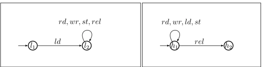
Example 2.1.2 (Mobile Reader). Consider reading e-books from an online store on tablet devices. A user, when reading an e-book, may write some annotations. The way of using the online store depends on which kind of connections, low-bandwidth or high-bandwidth, a tablet device has. In the former case, the tablet needs to load an e-book from the store to local memory before any other actions and if users make annotations on the e-book, it requires to store them back on the online store. In the latter case, the user directly reads/writes e-books, however it is required that the user eventually releases the connection due to the high cost of the connection. We use rd, wr, ld and st to model operations of reading e-books, writing annotations, loading e-books from the online store to local memory and storing them back to the online store, respectively. The action rel denotes the operation of releasing the connection.

We assume two tablet devices. Their specifications are given by the labelled transition systems in Fig. 2.1. The figure on the left corresponds to the first device, while on the right - the second device. The set A of actions is _{{rd, wr, ld, st, rel}.} The set of initial states is I = _{l1, h1}. The first device always loads e-books to

the local memory before any other actions, hence it satisfies the policy of the low-bandwidth connection. The second device intends to work with the high-low-bandwidth connection, since it guarantees read/write operations without loading e-books to its local memory. However, its infinite run without performing rel violates the policy of the high-bandwidth connection.

2.1.2 Automata and Languages

We define an automaton as a labelled transition system. Finite state automata are a class of automata, which is used in many different areas, including computer science,

(23)

2.1. PRELIMINARIES 23 l1 ld l2 rd, wr, st, rel h1 h2 rd, wr, ld, st rel

Figure 2.1: Transition systems of a mobile reader with a low-bandwidth (on the left) and a high-bandwidth (on the right) connection

mathematics and logics. In this text, we use them as a formalism to specify various properties of behaviour of computing systems (see below).

Definition 2.1.3 (Languages). Given a set A of actions. A finite trace over A is a finite sequence α1α2. . . αn, where αi ∈ A, 1 ≤ i ≤ n. A infinite trace over A is a

infinite sequence α1α2α3. . . , where αi ∈ A, 1 ≤ i. We use η, η" to range over traces

(both finite and infinite). A∗ _{denotes a set of all finite traces over A. A}ω _{denotes a}

set of all infinite traces over A and A∞ = A∗∪ Aω_{. A language over A is a subset}

of A∞_.

Given a labelled transition system LT S = (Q, A,_{→, I), each finite path of LT S} r = q0 α1 → q1 α2 → . . .αn → qn,

corresponds to a finite trace η = α1. . . αn (similarly for infinite executions). A trace

α1. . . αi, where i≤ n, is called a prefix of η. α1. . . αi, where i < n, is called a proper

prefix of η. We write pref (η) for a set of all finite prefixes of η, i.e. pref (η) =_{{ˆη|ˆη is a finite prefix of η}}

We use T races(q) to denote the set of traces generated by the executions starting from the state q of LT S and T races(LT S) =!_q_∈IT races(q).

Example 2.1.4. In the example of the mobile reader, ld.rd.rd.wr in the low-bandwidth connection or rd.ld.wr.rel in the high-low-bandwidth connection are possible traces.

Remark 2.1.5. By abuse of notation, we denote by η, η" both paths and traces (it will be clear from the context).

Definition 2.1.6 (Automata on finite traces). A finite state automaton (FSA)_{A is} a structure (Q, A,_{→, I, F ), where (Q, A, →, I) is a finite labelled transition systems,} where I ⊆ Q is the set of initial states and F ⊆ Q is the set of final states.

A run of a finite trace α1α2. . . αn ∈ A∗inA is a finite sequence of states q0q1. . . qn

such that r = q0 α1 → q1 α2 → . . . αn → qn

(24)

with qi αi+1

→ qi+1 for all 0 ≤ i ≤ n and q0 ∈ I. A run q0q1. . . qn is called accepting

if qn ∈ F . A finite trace α1α2. . . αn ∈ A∗ is called accepted if there is an accepting

run for it. We denote by L(A) the set of all accepted traces of A (sometimes called the language generated by_A).

Definition 2.1.7 (Regular Languages). A language over A is called regular if it is generated by a finite state automaton.

Informally, an FSA can recognise a set of finite traces, but not a set of infinite traces. In case of infinite traces, we need a different formalism.

Definition 2.1.8 (ω-Languages). Given a set of labels_{A, an ω-language is a subset} of Aω_.

Among ω-languages, the class of ω-regular languages enjoys many fundamental de-cision problems and has been successfully used in the specification and formal veri-fication of computing systems [8].

Definition 2.1.9 (ω-Regular Languages). For a regular language L_{⊆ A}∗_{, we define}

an ω-language Lω _{as the set of all infinite concatenations of traces in L, i.e.}

Lω =_{w1w2w3. . .|wi ∈ L, i ≥ 1}

An ω-language L_{∈ A}∞ _{is called ω-regular language if it has a form}

• L0ω, where L0 is a regular language.

• L1L2, the concatenation of a regular language L1 and an ω-regular language

L2, i.e. {w1w2|w1 ∈ L1∧ w2 ∈ L2}.

• L1∪ L2, the union of regular languages where L1, L2 are ω-languages.

Definition 2.1.10 (Automata on Infinite Traces). A Buchi automaton_{A is a} struc-ture (Q, A,_{→, I, F ), where (Q, A, →, I) is a finite labelled transition systems, where} I ⊆ Qis the set of initial states and F ⊆ Q is the set of final states.

A run of a infinite trace α1α2α3· · · ∈ Aω in A is infinite sequence of states

q0q1q2. . . such that r = q0 α1 → q1 α2 → q2 α3 → q3. . . with qi αi+1

→ qi+1for all 0 ≤ i and q0 ∈ I. A run q0q1q2. . . is called accepting if qi ∈ F

for infinitely many indices i_{∈ N . A infinite trace α}1α2α3· · · ∈ A∗ is called accepted

if there is an accepting run for it. We denote by L(A) the set of all accepted traces of _{A (sometimes called the language generated by A).}

A Buchi automaton is called deterministic if for each q ∈ Q and α ∈ A there is at most one q" such that q→ qα " _{∈→. Otherwise, it is called non-deterministic.}

Lemma 2.1.11 (ω-languages and Non-deterministic Buchi Automata ). The class of languages accepted by Non-deterministic Buchi Automata agrees with the class of ω-regular languages.

(25)

2.1. PRELIMINARIES 25

2.1.3 Properties of Computing Systems

For verification purpose, one needs to check some conditions in a given state or across a number of states of the transition system model of the computing system under consideration. These conditions are usually referred as properties of the sys-tem. Properties about a single state are called state-based, whereas properties about several successive states are called linear-time or path-based.

Example 2.1.12. In the mobile reader example, it is desirable to have the property that requires that whenever the mobile reader takes a high-bandwidth connect, it eventually releases it.

Here we consider two important classes of linear-time properties: regular safety properties and regular liveness properties. What make them interesting is that these properties can be checked in an automated manner [8], using decidable decision problems in the field of automata. Following formulation in [8], we define linear time properties as follows.

Definition 2.1.13 (Linear Time Properties). Given a set A of actions, a linear-time property P over A is a subset of Aω_.

Example 2.1.14. In the mobile reader example, a set of traces, which begin by an ld and are followed by infinite number of rd and wr, i.e. ld.(_{{rd, wr})}ω _{represents a}

possible linear time property.

Intuitively, a safety property asserts “that nothing bad will happen” during the evolution of the transition system. Here we consider regular safety properties, i.e., safety properties whose bad prefixes constitute a regular language, and hence this set can be represented by a finite state automaton.

Definition 2.1.15 (Safety Properties). A linear-time property Psaf e over A is a

safety property if for all traces η∈ Aω_{\ P}

saf e there exists a finite prefix ˆη of η such

that

Psaf e∩ {η" ∈ Aω|ˆη is a finite prefix of η"} = ∅

The prefix ˆη is called a bad prefix for Psaf e. A bad prefix for Psaf e is minimal if no

proper prefix of ˆη is a bad prefix for Psaf e. A safe property Psaf e is called regular if

the set of all its bad prefixes is a regular language.

Remark 2.1.16. Notice that a bad prefix ˆη of a linear-time property Psaf e could

be a prefix of many traces, which are not in Psaf e.

Lemma 2.1.17 (Criterion for Regularity of Safety Properties). A safety property Psaf e over A is called regular if its set of bad minimal prefixes constitutes a regular

(26)

Briefly, the algorithm to check a safety property Psaf e for a given finite transition

system relies on the reduction to the reachability problem in a product construction of the transition system with a finite automaton that recognises the bad prefixes of Psaf e. The reachability problem of the resulted automaton is then analysed. If a

final state is reachable, then the property does not hold in the transition system. (The interested readers are referred to [8] for more details).

A liveness property asserts that “something good eventually happens”, and is used mainly to ensure progress. For instance, in the example of the mobile reader with the low-bandwidth connection the property that requires that the action save is eventually reached after an occurrence of write.

Definition 2.1.18 (Liveness Properties). Given a set A of actions and a linear time property P over A, we write pref (P ) for!_η∈P pref (η). A linear-time property Plive

over A is a liveness property if pref (Plive) = A∗. A liveness property Plive is called

regular if it is recognized by a Buchi automaton.

In general, liveness properties are harder to verify than safety properties for a given finite transition system. However, one can use the same strategy for checking reg-ular safety properties to construct a product of the transition system with a Buchi automaton that recognizes Aω_{\ P}

live, then solve its reachability problem to check

whether a final state is reachable.

2.1.4 Temporal Logics

Temporal logics is a logical formalism suited for specifying linear time properties. The notion of time in temporal logics can be interpreted in either linear or branching view. In the linear view, at each moment there is a single successor moment, whereas in the branching view it has a branching, tree-like structure, where time may split into alternative courses. We follow the formulation introduced in [35].

Linear Temporal Logic There are many classes of temporal logics based on a linear-time perspective. We consider only Linear Temporal Logic (LTL), a variant of temporal logics. LTL is a powerful temporal logic, first introduced by Pnueli in [94], able to express many interesting properties of computing systems.

Definition 2.1.19 (Linear Temporal Logic). The LTL formulas over the set A of actions are defined by the following grammar:

ϕ ::= true | ¬ϕ | ϕ1∧ ϕ2 | (α)ϕ | ϕ1 U ϕ2,

where α_{∈ A.}

LTL includes the standard logical operators: conjunction ∧ and negation ¬. Note that the full power of propositional logic is obtained from them. LTL introduces two new modal operator: the next operator (α)ϕ and the until operator ϕ1Uϕ2.

(27)

Intuitively, (α)ϕ holds at the current state on a path if ϕ holds at the next state, which is a result of performing an action α, on the path, whereas ϕ1Uϕ2 holds on

a path if there is a future state on the path for which ϕ2 holds and ϕ1 holds until

that future state.

Convention 2.1.20. As usual, we write ϕ1 ∨ ϕ2 for ¬(¬ϕ1 ∧ ¬ϕ2), ϕ1 ⇒ ϕ2 for

¬ϕ1∨ ϕ2 and ϕ1 ≡ ϕ2 for ϕ1 ⇒ ϕ2 ∧ ϕ2 ⇒ ϕ1.

From the until operator we can derive two modal operators: F (“eventually”, some-times in the future) and G (“always”, from now on forever). Formally, they are defined as follows

F ϕdef= true Uϕ Gϕdef= ¬F ¬ϕ

Intuitively, F ϕ ensures that ϕ will eventually be true in the future and Gϕ holds if it is not the case that ¬ϕ will eventually true in the future, that is ϕ always holds. Other derived modal operators are the following:

never ϕ: G¬ϕ

infinitely often ϕ: GF ϕ

eventually forever ϕ: F Gϕ

every “request” will eventually lead to a “response”: G( request _{⇒ F response )} The formula G¬ϕ, where ϕ describes a bad behaviour, represents a safety prop-erty, while the others represent liveness properties. For instance, G( request ⇒ F response ) says that it is always true that whenever a request arrives, a response eventually replies.

Taking the linear view, LTL formulas stand for properties of paths. This means that a path can either fulfil an LTL formula or not. Technically speaking, the interpretation of an LTL formula is defined in terms of maximal paths or runs.

Before going into the details, we need some notations. Given a labelled transition system LT S and a path η = q1 → qα1 2 → qα2 3 → . . . of LT S, η(1) denotes the firstα3

state of η, i.e., q1, and η1 denotes the path q2 α2

→ q3 α3

→ . . . . Similarly, η(i) denotes the i-th state of η, i.e., qi, and ηi denotes the path qi

αi

→ qi+1 αi+1

→ . . . . With these notations, the denotation _{.ϕ. of a formula ϕ with respect to a labelled transition} system (Q,A, →, I) is .ϕ. = {η|η |=LT S ϕ}, where the relation |=LT S is inductively

defined by the following rules: η|= true

η_{|= ¬ϕ if η |= ϕ does not hold} η_{|= ϕ}1∧ ϕ2 if η|= ϕ1 and η |= ϕ2

η|= (α)ϕ if η(1)→ η(2) and ηα 2 _{|= ϕ}

η_{|= ϕ}1 U ϕ2 if ∃i : ηi |= ϕ2 and ∀j ≤ i : ηj |= ϕ1

Remark 2.1.21. Sometimes we also interpret an LTL-formula as the set of traces corresponding to its set of paths.

(28)

Definition 2.1.22. Given a transition system LT S, a state s of LT S satisfies an LTL formula, denoted by s _{|= ϕ, if P aths(s) ⊆ .ϕ. and LT S satisfies an LTL} formula, denoted by LT S _{|= ϕ, if for all initial states s}0 of LT S, s0 |= ϕ.

Automata-based LTL model checking. Now, we briefly describe a model-checking algorithm based on Buchi automata for LTL. Given a finite transition system LT S and an LTL formula ϕ that formalises a requirement on LT S, the problem is to check whether LT S _{|= ϕ . If it is refuted, an error trace needs to be} provided for debugging purposes. The counterexample consists of an appropriate finite prefix of an infinite trace in T S where it does not hold.

The model checking algorithm presented in the following is based on the automata-based approach as originally suggested by Vardi and Wolper in [106]. This ap-proach is based on the fact that each LTL formula ϕ can be represented by a non-deterministic Buchi automaton (NBA). The basic idea is to try to disprove LT S_{|= ϕ} by looking for a path η in LT S such that η|= ¬ϕ. If such a path is found, a prefix of η is returned as error trace. If no such trace is encountered, it is concluded that LT S _{|= ϕ.}

The essential steps of the model-checking algorithm rely on the following obser-vations:

LT S _{|= ϕ iff P aths(LT S) ⊆ .ϕ.}LT S

iff P aths(LT S)\ .ϕ.LT S =∅

iff P aths(LT S)_{∩ .¬ϕ. = ∅}

Hence, for NBA A with Lω(A) = .¬ϕ.LT S, we have LT S |= ϕ if and only if

P aths(LT S)∩ .¬ϕ. = ∅. Thus, to check whether ϕ holds for LT S one first con-structs an NBA for the negation of the input formula ϕ (representing the bad be-haviours) and then applies the techniques for the intersection problem (above). Computation Tree Logic. Branching time refers to the fact that at each moment there may be several different possible futures. Thus, the interpretation of formulas in branching time logics is defined in terms of an infinite, directed tree of states rather than an infinite sequence. Each traversal of the tree starting in its root represents a single path. The tree itself thus represents all possible paths, and is directly obtained from a transition system by unfolding at the state of interest. The tree rooted at state q thus represents all possible runs in the transition system that start in q.

In this text, we consider Computation Tree Logic (CTL), an expressive variant of branching time logics. The syntax of CTL formulas is given by the following definition.

Definition 2.1.23 (Computer Tree Logic). CTL formulas over the set A of actions are defined by the following grammar:

ϕ ::= true | ¬ϕ | ϕ1∧ ϕ2 | 1α2ϕ | E[ϕ1 U ϕ2]| A[ϕ1 U ϕ2],

(29)

In LTL, a formula holding in a state s requires that a formula ϕ holds in state s if all possible runs that start in s satisfy ϕ. Intuitively, we can state properties over all possible runs that start in a state, but not about some of such runs. CTL overcomes this by introducing the existential/universal quantification in the next and until operators, therefore CTL is able to specify such properties. More precisely, the prefixes E and A stand for the existential and universal quantification in their interpretations respectively.

The existential “eventually” EF and “always” EG operators can be derived from the until operator.

EF ϕdef= E[true Uϕ] EGϕdef= _{¬A[true U¬ϕ]}

Note that we also have their universal versions, i.e. [α]ϕ≡ ¬1α2¬ϕ, AF ϕ ≡ ¬EF ¬ϕ and AGϕ _{≡ ¬EG¬ϕ. The fragment of CTL containing the logical operators, the} existential next operator and the “eventually” EF (the “always” EG operator, resp.) is called the logic EF (the logic EG, resp.). The combination of the logics EF and EG yields the more expressive logic, called Unified System of Branching-Time Logic [20] (called the logic UB ). Let LT S = (Q, A,_{→, I) be a labelled transition system} with a set I of initial states. The denotation of a formula is a subset of states of LT S defined by the following rules:

.true.LT S = Q

.¬ϕ.LT S = Q\ .ϕ.LT S

.ϕ1∧ ϕ2.LT S =.ϕ1.LT S∩ .ϕ2.LT S

.1α2ϕ.LT S ={q ∈ Q|∃q" ∈ Q, (q, α, q")∈→ ∧ q" ∈ .ϕ.LT S}

.E[ϕ1 U ϕ2].LT S ={q ∈ Q|∃η ∈ P aths(q) such that

∃k ≥ 0.(∀0 ≤ j ≤ k.η(j) ∈ .ϕ1.LT S)∧ η(k) ∈ .ϕ2.LT S}

.A[ϕ1 U ϕ2].LT S ={q ∈ Q|∀η ∈ P aths(q) such that

∃k ≥ 0.(∀0 ≤ j ≤ k.η(j) ∈ .ϕ1.LT S)∧ η(k) ∈ .ϕ2.LT S}

Definition 2.1.24. Given a labelled transition system LT S = (Q, A,→, I), we say that a state q of LT S satisfies a CTL formula ϕ, denoted by q_{|= ϕ, if q ∈ .ϕ.}LT S.

We say that LT S satisfies a CTL formula ϕ, denoted by LT S _{|= ϕ, if I ⊆ .ϕ.}LT S

CTL model checking. The CTL model checking problem amounts to verifying for a given labelled transition system LT S and a CT L formula ϕ whether LT S _{|= ϕ.} A basic algorithm of CTL model checking is rather simple: (i) compute recursively a set .ϕ. of states satisfying ϕ; (ii) check whether I ⊆ .ϕ.. Alternatively, we can resort to the automata-based approach which is proposed in [73], which translates a CTL formula into an alternating tree automata and then reduces the problem to the non-emptiness problem of alternating tree automata.

(30)

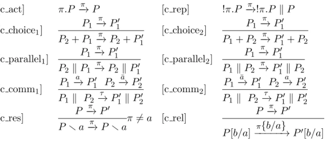
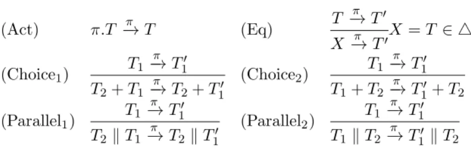
(Act) π.T −→ Tπ (Eq) T π −→ T" X₋_{→ T}π "X = T ∈ 4 (Choice1) T1 −→ Tπ 1" T2+ T1 −→ Tπ 2+ T₁" (Choice2) T1−→ Tπ 1" T1+ T2−→ Tπ ₁" + T2 (Parallel1) T1−→ Tπ 1" T2. T1−→ Tπ 2 . T₁" (Parallel2) T1 −→ Tπ 1" T1 . T2 −→ Tπ ₁" . T2

Figure 2.2: The Operation Semantics of BPP processes.

2.1.5 Basic Parallel Processes

Basic Parallel Process (BPP) [45] is considered as one of the most simplest models of concurrency. It contains the prefix action ., the choice operator + and the merge operator ..

Definition 2.1.25. We assume a set of process variablesPV, ranged over by X, Y, Z, a set A of actions, ranged over by α, and τ 5∈ A to denote an internal or unobservable action. BPP expressions are defined as follows

(BBP expressions) T, T" ::= 0|X|π.T |T + T"_{|T . T}"

(prefix actions) π, π" ::= τ|α

The 0 is the empty process, i.e. the process that does nothing. The prefix action π.T is a process that performs π and then behaves like T . The choice T1+ T2 represents

a process that behaves either as T1 or as T2. The process T1 . T2 is the parallel

composition of T1 and T2 executing independently in parallel.

A BBP process is defined by the finite family _{4 of recursive process equations:} {Xi = Ti.1 ≤ i ≤ n},

where the Xi are distinct and the Ti are BPP expressions at most containing the

variables _{X1, . . . , Xn}. The variable X1 is singled out as the leading variable and

X1 = T1 is called the leading equation. The set of BPP processes is denoted byPbpp

A BPP expression T is called guarded if every variable occurrence in T is within the scope of action prefix sub-expression π.T" _{of T .}

A given finite family _{4 of guarded BPP equations determines a labelled} tran-sition system. The operational semantics of BPP processes is defined through the least transition relation satisfying the rules in Fig. 2.2.

Decidability of model checking BPP processes against linear time logics. Despite of its simplicity, BPP lies at the border of decidability of many model check-ing problems [78]. In [54], it is showed that model checkcheck-ing BPP with most branchcheck-ing time logics is undecidable. This follows from the result that model checking BPP

(31)

2.2. THE λ-CALCULUS 31

BPP general fixed formula

reachability NP-complete _{∈ NP}

EF decidable, PSPACE-complete ∈"pd

EG undecidable undecidable

UB undecidable undecidable

CTL undecidable undecidable

alternation free modal µ calc undecidable undecidable

modal µ calc undecidable undecidable

LTL decidable, EXPSPACE-hard decidable

linear time µ calc decidable, EXPSPACE-hard decidable Table 2.1: BPP decidability

with EG-fragment of CTL is undecidable. EF is the only decidable fragment of CTL for BPP. It has been showed that model checking BPP with EF-fragment is PSPACE complete. Model checking BPP for linear time logics is decidable and EX-PSPACE hard. The table 2.1 shows the complexity of model checking BPP (taken from [54]).

2.2 The λ-Calculus

The λ-calculus is a formal language introduced by Church in the 1930s to investigate functions, function applications and recursion. In spite of its very simple syntax, the λ-calculus is strong enough to describe all mechanically computable functions.

2.2.1 Syntax

Definition 2.2.1. Given an infinite set of variables _{V, ranged over by x, y, z. The} set E of λ-expressions, ranged over by e, e", is defined by the following grammar:

e, e" _::= _expressions

| x variable

| λx. e abstraction | (e1 e2) application

The values v, v" _{of the calculus are variables and lambda abstractions. , i.e.}

v, v" _::= _values

| x variable | λx. e abstraction

Definition 2.2.2. An occurrence of a variable x inside a term of the form λ.x e is said to be bound. The corresponding λx is called a binder, and we say that the

(32)

subterm e is the scope of the binder. A variable occurrence that is not bound is free. More generally, the set of free variables of a term e is denoted fv(e), and it is defined formally as follows

fv(x) =_{x}

fv(λx. e) = fv(e)\ {x} fv((e1 e2)) = fv(e1)∪ F V (e2)

An expression e is called closed if F V (e) is empty. We denote a set of closed λ-expressions as E0.

Convention 2.2.3. We often write let x = e1 in e2 for (λx. e2) e1, λ e for λx. e,

where x_{5∈ fn(e) and e}1; e2 for (λ e2) e1.

For any e, e" and x, substitution of e for x in e" is an operator for replacing every occurrence of x in e" _{by e with changing bound variables to avoid clashes. Formally,}

it is defined as follows.

Definition 2.2.4. A substitution of e for x in e"_{, denoted by e}"_{{e/x}, is defined as:}

x_{e/x} = e

(e1 e2){e/x} = e1{e/x} e2{e/x}

(λx. e"₎_{{e/x} = λx. e}"

(λy. e"₎_{{e/x} = λy. e}" _{if x}_{5∈ F V (e}"₎

(λy. e"){e/x} = λy. e"_{e/x} _{if x}_{∈ F V (e}"_{) and y} _{5∈ F V (e)}

(λy. e"₎_{{e/x} = λz. e}"_{{z/y}{e/x} if x ∈ F V (e}"_{), y} _{5∈ F V (e) and z 5∈ F V (e) ∪ F V (e}"₎

Definition 2.2.5. Let a λ-expression e contain an occurrence of λx. e", and let y 5∈ e"_{. We define α-conversion of e to e}"_{, denoted by e}_≡

αe", as a process that

replaces a sub-expression λx e"" _{of e by λy e}""_{{y/x}, where y does not occur at all in}

e.

Lemma 2.2.6. α-conversion is an equivalence relation.

Convention 2.2.7. From now on, unless stated otherwise, we identify λ-expressions up to α-conversion.

2.2.2 The operational semantics

The semantics of λ-expressions are defined through the concept of β-reduction, which captures the idea of function application. Formally, β-reduction is defined in terms of substitution.

Definition 2.2.8 (β-reduction). Any expression of the form (λx. e) e" _{is called a}

(33)

β-reduction to be the smallest relation→β on λ-expressions satisfying:

[β] λx.e e" →β e{e"/x} [cong1] e1→βe"1 e1 e2→βe"1 e2 [cong2] e2→βe"2 e1 e2→βe1 e"2

Call-by-value semantics. There are several strategies of β-reduction, which are based on different order of evaluation. In this text, we consider only call-by-value strategy. Intuitively, call-by-value order is defined as “only outermost redexes are reduced”, and “a redex is reduced only when its right-hand side has already been reduced to a value”. For more details, we refer the reader to [92].

Definition 2.2.9. We define a call-by-value β-reduction to be the smallest relation →βcbv on λ-expressions satisfying: [cbv β] λx.e e" _→ βcbv e{e"/x} [cbv cong1] e1→βcbve"1 e1 e2→βcbve"1 e2 [cbv cong2] e2→βcbve"2 v e2→βcbvv e"2

And, e→βcbve" if and only if e" is obtained from e by a single β-reduction. We

write_{→ for →}βcbv, unless stated otherwise. Moreover,→∗ denotes the reflexive and

transitive closure of→.

Notice that in the rule [cbv cong2], the first term of application in the conclusion is

always a value.

Definition 2.2.10. Applicative Bisimulation A binary relation R on E0 is a

simulation if whenever e R d and e →∗ _λx.e"_{, then there exists d}" _{such that d} _→∗

λx.d"_{, λx.e}" _{R λx.d}" _{and for any value v, e}"_{{v/x} R d}"_{v/x}.

We write! for the union of all simulations and call it similarity. A binary relation R on T0 is a bisimulation if R and its conversion R−1, i.e. R−1 ={(e2, e1)|(e1, e2)∈ R} ,

are simulations. We write_{∼ for the union of all bisimulations and call it bismilarity.} Definition 2.2.11. An equivalent relation R on T0 is a congruence if it is preserved

by the operations and substitutions.

In [61], Howe showed that bisimilarity is a congruence. Theorem 2.2.12. Bisimilarity _{∼ is a congruence relation.}

(34)

2.2.3 Control Flow Analysis

Since introduced in the sixties [96], Control Flow Analysis (CFA) has proved its im-portance in the cycle of development of software. Basically, it provides a framework to compute which values or information can reach certain program points or can be assigned to a specific variable. Control Flow Analysis comes into many different formulations, as stated in [86], such as constraint-based, abstract interpretation-based and specification-interpretation-based, and type-interpretation-based. The simplest form of Control Flow Analysis is so-called 0-CFA, which does not take the context information into ac-count when analysing programs. Intuitively, it does not distinguish instances of function calls, more precisely, different instances of program points and variables of the function at various call sites.

In this section, we consider specification-based approach to 0-CFA for a simply typed calculus, based on [86]. To consider this approach, the syntax of the λ-calculus is extended with recursive variable, which are bound to function bodies. Definition 2.2.13. Given an infinite set of variables_{V, ranged over by x, y, z. The} set E of λ-expressions, ranged over by e, e"_{, is defined by the following grammar:}

| x variable

| λzx. e abstraction

| (e1 e2) application

The values v, v" _{of the calculus are variables and lambda abstractions. , i.e.}

v, v" _::= _values

| x variable

| λzx. e abstraction

The set of free names and notion of substitution are defined as expected. The operational semantics of extended λ-expressions is similar to the one defined in the previous section, except that the rule [cbv β] is defined as follows:

[cbv β] λzx.e e" →βcbv e[λzx.e/z, e"/x],

where e[λzx.e/z, e"/x] is a simultaneous substitution. The idea is that the recursive

variable is replaced by the function body λzx.e when reduction is applied.

Also, given λ-expression e, assume that all program points (i.e all sub-expressions of e) are labelled and, for simplicity, all labels are just integers. We denote the set of all labels by Lab, ranged over by l and the set of extended λ-expressions by E∗, ranged over by t. Formally, we define the following abstract syntax:

l ∈ Lab labels t ::= el_{, where e}_{∈ E} _terms

(35)

The result of 0-CFA analysis is a pair of (C, ρ) where C is a mapping from program points to a set of values, i.e. C(l) contains the values, i.e. variables or lambda abstractions, that can reach the program point l and ρ(x) is mapping from variables to a set of values, i.e. ρ(x) contains the values that the variable x can be bound to. Formally, C is a mapping from labels to sets of values and ρ is a mapping from variables to sets of values.

Example 2.2.14. As a running example, we use the following λ-expression: e = let g = (λfx. (f1 (λy. y2)3)4)5 in (g6 (λz. z7)8)9

The idea behind Control Flow Analysis is that based on control flow it defines rules for transferring all possible information from one program point to another. Usually, this set of rules forms a specification of analysis. The specification is defined in Tab. 2.2. To specify Control Flow Analysis, we firstly use the specification to generate a system of constraints and then find a solution of the system. It leads to the following definition.

Definition 2.2.15. A pair of (C, ρ) is an acceptable 0-CFA analysis of a λ-expression e if it satisfies the system of constraints generated by specification when analysing e, where constraints are defined as follows:

• C(l) ⊆ ρ(x), that is, a set of values that reach the program point labelled by l is included in the set of values that are possibly bound to the variable x. • C(l) ⊆ C(l"_{), that is, a set of values that reach the program point labelled by}

l is included in the set of values that reach the program point labelled by l". • S ⊆ ρ(x), that is, a set S of values is included in the set of values that are

possibly bound to the variable x.

(abs) (C, ρ) _{|= (λ}zx. e)l iff {λzx. e} ⊆ C(l) ∧ (C, ρ) |= e

(app) (C, ρ) |= ((e1)l1 (e2)l2)l iff (C, ρ)|= (e1)l1∧ (C, ρ) |= (e2)l2

∧ (∀(λx. e0l0)∈ C(l1)) : (C, ρ)|= e0l0 ∧ C(l2)⊆ ρ(x) ∧ C(l0)⊆ C(l)

∧ (∀(λzx. e0l0)∈ C(l1)) : (C, ρ)|= e0l0 ∧ C(l2)⊆ ρ(x) ∧ C(l0)⊆ C(l)

∧ {λzx. e0l0} ⊆ ρ(z)

Table 2.2: Specification of 0-CFA

In the rule (abs), the analysis holds for the sub-expression e and the abstraction λzx e is included in a set of values reaching the label l. The rule (app) not only

(36)

each reachable abstraction-value λzx.t0l0 at l1, that is: i) a set of values reaching the

label l2 can be bound to x; ii) a set of values reaching the label l contains a set of

values reaching the label l0; iii) in the case of recursive abstraction-values, the value

is bound to its recursive variable.

Example 2.2.16. We apply the CFA to our example. The system of constraints is generated as follows: (1) (_{∀(λx. e}0l0)∈ C(5)) : (C, ρ) |= e0l0 ∧ C(8) ⊆ ρ(x) ∧ C(l0)⊆ C(9) (2) (∀(λzx. e0l0)∈ C(5)) : (C, ρ) |= e0l0 ∧ C(8) ⊆ ρ(x) ∧ C(l0)⊆ C(9) ∧ {λzx. e0l0} (3) (_{∀(λx. e}0l0)∈ C(1)) : (C, ρ) |= e0l0 ∧ C(3) ⊆ ρ(x) ∧ C(l0)⊆ C(4) (4) (∀(λzx. e0l0)∈ C(1)) : (C, ρ) |= e0l0 ∧ C(3) ⊆ ρ(x) ∧ C(l0)⊆ C(4) ∧ {λzx. e0l0} (5) _{{f} ⊆ C(5)} (6) ρ(f ) ⊆ C(1) (7) _{idy} ⊆ C(3) (8) ρ(y)_{⊆ C(2)} (9) {idx} ⊆ C(8) (10) ρ(z)_{⊆ C(7)}

where f = λfx. (f1 (λy. y2)3)4, idy = λy. y2 and idz = λz. z7. In this system,

the first four constraints are conditional or implicit constraints, which are generated when analysing the λ-expressions at the labels 9 and 5. More precisely, in (1) and (2), for each reachable abstraction-value λzx. e0l0 at the label 5: i) all

abstraction-values reaching at the label 8 are included in the set of abstraction-values bound to x; ii) all abstraction-values reaching at the label l0 are also reached at the label 9. iii) all

recursive abstraction-values are bound to its recursive variable. Similar arguments can made for clauses (3) and (4). The remaining constraints from (4)-(18) are called explicit constraints, which relate values to their labels.

One of solutions of the above systems is the following:

C(1) = {f} C(2) = ∅ ρ(f ) = {f}

C(3) = _{idy} C(4) = ∅ ρ(g) = {f}

C(5) = _{f} C(6) = _{f} ρ(x) = _{idy, idz}

C(7) = ∅ C(8) = {idz} ρ(y) = ∅

C(9) = _∅ C(10) = _∅ ρ(z) = _∅

Theoretical properties. The proof of existence of acceptable 0-CFA analysis is given in literature, see [86] for details. Moreover, the solution is not unique. For example, by taking the above solution and adding more information to C(5), C(6)

(37)

2.2. THE λ-CALCULUS 37 as follows: C"_{(5) =} _{{f, id} y} C"_{(6) =} _{{f, id} z}

C"(i) = C(i), where i5= 5, 6

We have another acceptable analysis (C"_{, ρ), but less precise. Theoretically, a set}

of acceptable analyses for a specific term enjoys the model intersection property, i.e. whenever we take the intersection of a number of acceptable analyses we still get an acceptable analysis. As a consequence, we can obtain the least (most precise) solution from the set of acceptable analyses for the term.

Definition 2.2.17. The set of acceptable analyses can be partially ordered by set-ting (ρ, C)_{7 (ρ}"_{, C}"_{) if and only if} _{∀l ∈ Lab, C(l) ⊆ C}"_{(l) and} _{∀x ∈ V, ρ(x) ⊆ ρ}"_(x).

We write (ρ, C)8 (ρ"_{, C}"_{) ((ρ, C)}_{9 (ρ}"_{, C}"_{), resp.) for the binary least upper bound}

( the binary greatest lower bound, resp.) (defined point-wise). We use _{8I (9 )to} denote the least upper bound ( the greatest lower bound, resp.) for a set I of acceptable analyses.

The important feature of a Moore family set is that it enjoys the model intersection property.

Definition 2.2.18. The set of estimates is a Moore family if and only if it contains 9J for all J ⊆ I.

Theorem 2.2.19 (Existence of the least solution). Given a λ-expression e, a set of acceptable analyses of e, i.e. {(C, ρ)|(C, ρ) |= e}, is a Moore family.

More importantly, the least acceptable analysis is correct with respect to the seman-tics, i.e. it ensures that the information from the analysis is indeed a safe description of what will happen during the execution of the program.

Theorem 2.2.20 (Subject Reduction). Given a λ-expression e, (C, ρ) _{|= e. If} e_{→ e}"_{, then (C, ρ)}_{|= e}"_.

Remark 2.2.21. We refer readers to [86] for details of he algorithm of computing the least solution of a system of constraints.

2.2.4 The λ

[]

-calculus

We present an extension of the simply typed lambda calculus, called lambda box (λ[]_{), with possible expressing resources and events. This extension is introduced}

in [11] to formalise a model of history-based access control. The idea behind it is to abstract the entire execution by means of sequences of events, called histories, and to specify access control for running code based on these histories generated by the code so far. By considering the entire execution, it improves the idea of e.g. stack inspection [57], which instead records a fragment of the whole execution,

(38)

hence provides a better understanding of the behaviour of programs. Indeed, the previous analysis originally comes from the idea of history-based access control. It is simple to approximate all the possible runtime histories of the programs and then use some model checking to check whether the resulting approximations satisfy some policy based on the sequence of events.

The Syntax

Definition 2.2.22. (Local Policies) Let A be a set of actions, a policy ϕ is a regular safety property over A.

Definition 2.2.23. Let V be an infinite set of variables, ranged over by x, y, z, R be a set of resources, ranged over by r, r"_{, and A be a set of monadic actions, ranged}

over by α, β. A set Ev of access events is defined as _{{α(r)|α ∈ A and r ∈ R}. We} assume a set Φ of local policies, ranged over by ϕ, ϕ". The set E[] _{of λ}[]_{-expressions,}

ranged over by e, e"_{, is defined by the following grammar:}

| x variable

| α(r) access event

| if b then e1 else e2 conditional

| λz x. e abstraction

| (e1 e2) application

| ϕ[e] policy framing,

The values v, v" of the calculus are variables and lambda abstractions, i.e. v, v" _::= _values

| x variable

| λz x. e abstraction

We write 0 for a fixed, closed and event-free value. The definition of guards b in conditionals is irrelevant here, and so it is omitted.

The language λ[] _{extends the λ-calculus by adding two new language constructs.}

The first one is that of access events α(r), which describes the application of the action α on the target resource r at runtime. A finite sequence of access events is called a history. The second one is that of policy framing ϕ[e] which indicates that the evaluation of e must obey the policy ϕ.

Usage Automata. Security policies ϕ_{∈ Φ are modelled as regular safety properties} of histories, i.e. properties whose set of bad prefixes are recognized by an automaton, as discussed above. A policy framing ϕ[e] enforces regular property of histories during the execution of e. The policy ϕ can be represented by the set of its bad prefix, which in turn is recognized by usage automata introduced in [10]. Here

(39)

2.2. THE λ-CALCULUS 39 q1 q2 q3 ld rd, wr, st, rel rd, wr, st, rel

Figure 2.3: The usage automata for the policy of the low-bandwidth connection we consider a simplified version of usage automata, where usage automata do not contain resource variables. We refers readers to [10] for more details. Informally, a usage automaton describes a policy defined by a regular safety property. Usage automata are considered as an extension of automata, where its final states are offending, entering into which is considered as a policy violation. We write η |= ϕ if the history η does not lead to offending states in the corresponding usage automaton. Example 2.2.24. Back to our reader mobile example, it could be required that for the low-bandwidth connection the tablets needs to load an e-book to local memory before any other actions. The usage automata given in Fig. 2.3 describes this policy. The set Q of states is{q1, q2, q3} and the set A of actions is {rd, wr, ld, st, rel}. The

only final state q3 is marked by a double circle, which indicates the offending state.

At the beginning, from the initial state q1 any action, except for ld, leads to the

offending state q3, which therefore describes the required policy.

The Operational Semantics. The behaviour of λ[]_{-expressions, described in}

Fig. 2.4, is defined through a structural operational semantics. A transition (η, e)_→µ (η"_{, e}"_{), indicates that, starting from a state described by the history η, the}

expres-sion e evolves to e", issuing an event µ, possibly extending the history to η". Initial configurations have the form (*, e), where * denotes the empty history.

[s event] η, α(r)→ ηα(r), 0 [s app0] η, (λzx.e) v → η, e[λzx.e/z, v/x]

[s cond0] B(b) = true η, if b then e1 else e2 → η, e1 [s cond1] B(b) = false η, if b then e1 else e2 → η, e2 [s app1] η, e1 → η, e"1 η, e1 e2 → η, e"1 e2 [s app2] η, e2 → η, e"2 η, v e2 → η, v e"2 [s pol0] η, e_{→ ηα(r), e}" _ηα(r)_{|= ϕ}

η, ϕ[e]→ ηα(r), ϕ[e"_] [s pol1]

η_{|= ϕ} η, ϕ[v]→ η, v

A Language-based Approach to Distributed Resources

Dipartimento di Informatica

Dottorato di Ricerca in Informatica

INF 01

Ph.D. Thesis

A Language-based Approach to

Distributed Resources

Viet Dung Dinh

Abstract

Acknowledgments

Contents

I

A Model of Cloud Systems

59

II

Static Analysis for Distributed Resources

83

List of Figures

List of Tables

Chapter 1

Introduction

1.1

Motivations

1.2

Structural Operational Semantics

1.3

The λ-calculus

1.4

Process Algebras

1.5

Static Program Analysis

1.6

Contributions

1.7

Outline of the Work

1.8

Origins of the Chapters

Chapter 2

Background

2.1

Preliminaries

2.1.1

Transition Systems

2.1.2

Automata and Languages

2.1.3

Properties of Computing Systems

2.1.4

Temporal Logics

2.1.5

Basic Parallel Processes

2.2

The λ-Calculus

2.2.1

Syntax

2.2.2

The operational semantics

2.2.3

Control Flow Analysis

2.2.4

The λ

-calculus